Systematic Analysis of Geo-Location and Spectrum Sensing as Access Methods to TV White Space

Hope Mauwa^1,*, Antoine Bagula¹, Marco Zennaro², Ermanno Pietrosemoli², Albert Lysko³ and Timothy X. Brown⁴

¹University of the Western Cape, ISAT Lab, Dept. of CS, Bellville, South Africa
²International Centre for Theoretical Physics, ICT4D Laboratory, Trieste, Italy
³Meraka Institute, Council for Scientific and Industrial Research, Pretoria, South Africa
⁴Carnegie Mellon University, Department of Engineering and Public Policy, Kigali, Rwanda

E-mail: {hmauwa; abagula}@uwc.ac.za; {mzennaro; ermanno}@ictp.it; alysko@csir.co.za; timxb@andrew.cmu.edu

*Corresponding Author

Received 28 February 2017;
Accepted 8 March 2017

Abstract

Access to the television white space by white space devices comes with a major technical challenge: white space devices can interfere with existing television signals. Two methods have been suggested in the literature to help white space devices identify unused channels in the TV frequency band so that they can avoid causing harmful interference to primary users; geo-location spectrum database and spectrum sensing. Discussions in the literature have placed much emphasis on the limitations of the spectrum sensing approach mainly from the perspective of the developed world environment in which its drawbacks are significant. Little attention has been placed to the limitations of the geo-location database approach when applied in a developing regions. This paper considers a broader analysis of the approaches by looking at factors that can affect their performance and how the presence or absence of these factors in a developed region or developing region can affect their applicability. In so doing, the paper highlights the need to conduct more research on the performance of spectrum sensing in developing regions where there are much less TV broadcasting stations and therefore, white spaces are more abundant.

Keywords

Geo-location database
spectrum sensing
performance factors
best approach

1 Introduction

The radio frequency spectrum is a limited resource and most of the useful part is already allocated to different wireless services. As a result, it is now becoming difficult to find useful vacant bands to either deploy new wireless services or enhance the existing ones [1]. The scarcity of the radio frequency spectrum scarcity has the potential to hinder the development of future wireless communication systems [2, 3] if alternative means of sharing the already allocated useful part of the radio frequency spectrum is not found. Faced with the limitation of the natural radio frequency spectrum and the increase in demand for it, work is being carried out by research institutions and other stakeholders to find new and innovative techniques that can offer ways of sharing the already allocated radio frequency spectrum. In this quest, government institutions, research institutions, and other stakeholders around the world have performed measurements and studied the occupancy of the already allocated part of the radio frequency spectrum. The measurements have revealed that most of the allocated radio frequency spectrum is heavily underutilized except for the radio frequency spectrum allocated to cellular technologies, and the Industrial, Scientific and Medical (ISM) bands [4]. The underutilization is more apparent in the TV broadcasting frequency band where it has shown to be unused [5–8] most of the time. These unused radio frequency spectrum in the Ultra High Frequency (UHF) TV radio frequency band (so called TV white spaces) have been suggested as the solution to meet the growing demand for the wireless data transmission and have the potential to boost broadband communication in both rural and urban areas to support applications that can benefit communities such as drought mitigation [9, 10], community healthcare [11, 12], smart parkings [13], and many others. An efficient long-term solution that has been proposed for accessing the radio frequency spectrum is dynamic spectrum access (DSA) [14], in which devices are able to make real-time adjustment of spectrum utilization in response to changing environment using cognitive radio (CR) technology. Currently, CR technology has not been adopted yet as the technical details for its implementation have not been completely solved. The TV broadcasters are primary users (often called incumbents) in the frequencies bands allocated to them in each country, and therefore, any secondary user (like the TV white space devices) of these bands must provide assurances that will not cause interference to the primary user (the TV broadcasting receiver).

Detecting the TV white spaces (TVWSs) or vacant channels in the TV radio frequency band is difficult as the vacant channels vary according to location and time of the day. This places a ‘must do’ requirement on any secondary user device to check if a primary user signal is present in a channel before it goes ahead using it. Two techniques have been suggested in the literature to help white space devices (WSDs) do this: geo-location spectrum database and spectrum sensing. Discussions in the literature, which are based mainly on the developed world environment, have placed much emphasis on the limitations of the spectrum-sensing approach. This may have been the case because the idea to use TV white space (TVWS) originated from the developed world and the initial experiments were conducted there. Some performance requirements specific to developing countries have not been discussed in the literature clearly. The presence or absence of these requirements in a region could potentially affect their performance. This paper considers a broader analysis of each approach by looking at factors that can affect their performance in developing region.

The rest of the paper is structured as follows; Section 2 gives a general discussion of the two approaches. This is followed by a discussion of the relevant performance factors of the approaches, provided in Section 3, and a discussion of what is considered to be the best approach, in Section 4. Section 5 provides evaluation of the approaches by comparing path losses derived from measurement data versus predicted path-loss values of some propagation models being suggested for used in geo-location databases. Section 6 compares our experiment with similar experiments conducted in other countries in terms of equipment used and the results obtained and Section 7 concludes the paper.

2 Detection Techniques

Two approaches have been proposed to allow WSDs assess the available TVWS in the TV frequency band. The first approach relies on a database with information about known primary transmitters and the application of some propagation loss model to predict the value of the primary user signal at any given point in time (geo-location spectrum database approach). An alternative is to use one device or a network of devices to physically scan the radio waves to detect the presence of TV signals (spectrum sensing approach).

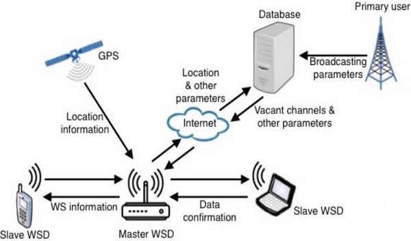
Figure 1 Geo-location database implementation.

2.1 Geo-Location Spectrum Database

Figure 1 shows a simple implementation of the geo-location database approach. The approach requires a white space device (WSD) to send a query to a geo-location database of known TV transmitters in order to determine the available spectral opportunities at a given location. Before the WSD can query a geo-location database it needs to be authenticated first by registering with the database. After registering with the database, the WSD can now query the database for available channels by sending its location, demand, and other optional information such as device type and location accuracy [15] to the database. The WSD determines its location through a geographical positioning system (GPS) or via a base station that it is associated with [16]. The database responds to the WSD query with details of available white spaces (e.g., frequencies and transmission power limits) at the WSDs location [15]. The WSD selects a channel for its operation (or it decides not to select any channel) and inform the database about its selection by sending the number of the selected channel and information about itself such as device type and number, transmit power, etc., [17] to the database. The database then register the WSD (if necessary) and indicates that the selected channel is used by the particular WSD [18]. All this communication happens over the Internet, thus imposing a significant limitations to places where Internet access is poor. The database is also dynamically updated over the Internet with the incumbents information so that the information it contains remains valid.

To identify white spaces over the TV frequency bands, the geo-location database stores a set of transmission parameters of known TV transmitters and their primary operational characteristics and translates that information into a list of allowed frequencies and associated transmit powers to the WSD [18] using propagation models. Some of the primary TV transmitter operational characteristics stored by the database include location, antenna parameters (radiation pattern, height), transmit power, times of operation, protection requirements, frequency of operation and other related parameters. The propagation models can be statistical, based only on distance and frequency, or they can based on ray tracing techniques that require detailed information about the terrain elevation in the area of interest. Therefore, correct identification of the presence of a TV signal at a given location depends on the fidelity of the database information and quality of the propagation model used to predict signal coverage [14].

2.2 Spectrum Sensing

Sensing the spectrum using a detector is another method of determining spectrum availability. In this approach, the detector does not know any information about the locations of TV transmitters and their transmission powers. The protection of the TV user is estimated from the measurements; if the measured signal level is so low to make it unusable by a TV receiver, the spectrum is assumed to be free, and therefore, available for secondary users can for TVWS transmission [19, 20].

In general, sensing methods can be divided into two categories: energy detection and feature detection. The energy detection can be performed with a spectrum analyzer like the Radio Frequency (RF) Explorer (see Figure 2), while feature extraction is based on specific characteristics of the type of signal to be detected and is therefore, more sensitive but also more complex. With the appropriately detection threshold, the secondary user can identify TVWSs accurately and be able to transmits in those bands without causing interference to the primary users [14]. Energy detection is the commonly proposed method due to its simplicity. It works by measuring the energy contained in a spectrum band and then comparing that with a set threshold value. If the energy level is above the threshold value, then the primary user signal is considered present otherwise the spectrum band is considered vacant.

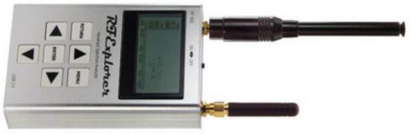
Figure 2 RF explorer.

3 Relevant Performance Factors

The optimal performance of each approach is dependent on the presence or absence of certain factors the will be discussed in the next section. The list may not be exhaustive and only includes factors deemed relevant to this discussion.

3.1 Performance Factors: Geo-Location Database Approach

An overview of the geo-location database approach is provided in Figure 3, which includes the factors deemed to be relevant to its performance. These factors must be present to optimize its performance.

3.1.1 Propagation models

The statistical propagation models are empirical models based on extensive measurements taken in real environments [21, 22]. Their predictions are more accurate if they are used in the environments in which they were developed for and in other similar environments. In those environments, the prediction results are close to ground truth, i.e. measured data. However, any propagation model is affected by different factors, for example, terrain elevation, terrain shapes, and environment changes [23], and as such, their accuracy in predicting signal attenuation over distance suffers greatly when they are used in environments other than the ones they were initially built for [24, 25]. So a ray tracing propagation model that uses elevation information and local terrain environment can be better in arbitrary locations [23].

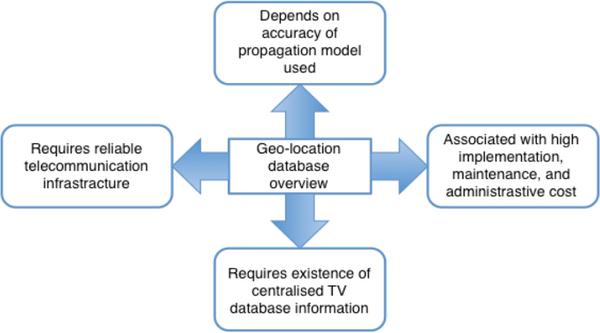
Figure 3 Overview of geo-location database approach.

3.1.2 Internet backbone infrastructure

Efficient and frequent communication between WSDs and the geo-location database is required in the database method if interference to incumbent is to be avoided. The master WSD must be able to determine its geographical position, which is often obtained by fitting it with a GPS receiver as depicted in Figure 1. The primary incumbent must also be able to send updated information about their broadcasting usage to the database. This means that the WSD must have a way to communicate to the database server before being able to use the TV frequencies. This implies the requirement of an alternate communication system, which adds complexity and cost to the device. Data connectivity is an issue in most developing world countries especially in the rural areas.

3.1.3 Existence of detailed TV database information

The fidelity of TV database information also plays a role in the correct identification of the presence or absence of a TV signal at a given location. Unavailability of nationwide transmitter information such as location, output power, antenna height and radiation pattern, etc., can limit the use of geo-location database approach. Spectrum regulators in many countries, especially in developing regions, often lack this detailed information. Furthermore, information regarding spectrum usage in neighbouring countries is required to assess spectrum occupancy in areas close to international borders. This entails another layer of complexity, requiring exchganging information among government agencies from different countries.

3.2 Performance Factors: Spectrum Sensing Approach

An overview of spectrum sensing approach is provided in Figure 4. It summarizes the factors that affect its performance, which are discussed in more detail in subsequent subsections.

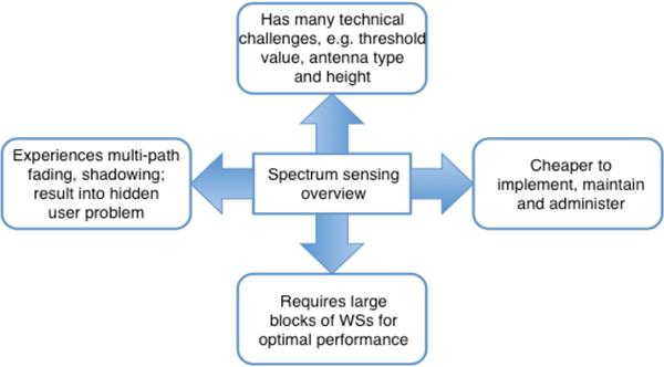
Figure 4 Overview of spectrum sensing.

3.2.1 Multi-path fading and shadowing

Signals experience multi-path fading and shadowing due to obstacles in their path such as buildings as they propagate through the wireless medium. Such effects may lead to a scenario called the hidden user problem or hidden terminal problem [26] where a WSD is unable to detect the presence of a primary signal in a channel. This could happen for instance if the sensing device is indoors at ground level, where the signal is lower than the one that could be captured by an external TV antenna on a roof. This leads to misinterpretation of measured data by the WSD which could start to transmit, causing interference to the primary user. These effects can be severe in places where there are a lot of obstacles such as tall buildings or hills.

3.2.2 Detection threshold

The value chosen as the detection threshold has a major impact on the performance of spectrum sensing equipment. If the value is too high, the technique fails to detect the presence of a TV signal in a channel thereby causing harmful interference to the incumbent, and if the value is too low, it results into false detection due to the ever present electromagnetic noise, when actually there is no TV signal in the channel, precluding the use of an available resource. The challenge is to come up with a threshold value that is optimal such that there is no harmful interference to the primary users or any missed opportunities by secondary users. Often there is no threshold that simultaneously gives low false positives and low false negatives. The Federal Communications Commission (FCC), the US regulator, mandates a sensing sensitivity threshold of -114 dBm by WSDs, which is considered as way too conservative by many in the literature and leads to waste of TVWS as well as increased complexity in the sensing device [4, 23, 27, 28]. In terms of protecting primary TV services from interference, higher threshold values might be cause of interference while lower threshold values lead to inefficient spectrum utilization.

4 So, What Is the Best Approach?

Since optimal performance of each approach is dependent on some factors that may not be present in some regions, neither approach can produce superior performance in all possible regions. For example, in regions or countries where propagation models have been tried and tested extensively such that their prediction results are close to ground truth data, there is reliable Internet backbone infrastructure and a centralized detailed TV database information is also available, the geo-location database approach is expected to perform better than spectrum sensing. That could be the case with developed regions such as the US and Europe where all the three factors are present. It is therefore not surprising that the geo-location database approach is being given preference as the main technique of finding TV white spaces [29–32] in those regions. However, conditions in developing regions are quite different from developed regions. Internet backbone infrastructure is poor and unreliable, especially in the rural areas; propagation models have rarely been tested there so that their behaviour is unclear at the moment; spectrum usage information is scattered and stored in many formats, electronic and paper, and the regulators have not collected it into a useful centralized database that is publicly available.

Therefore, when these conditions prevail, the use of a geo-location spectrum database approach may not produce optimal results.

Fading, shadowing and the hidden user problem, relevant to spectrum sensing, can be severe in the developed world because of many tall buildings, which are also close together. Consequently, primary TV signals are difficult to detect accurately by spectrum sensing alone and could result in harmful interference to users who have deployed TV receiving antennas in the top of their buildings. Therefore, performance of spectrum sensing in urban areas may be low. On the contrary, rural areas, especially those of developing world countries, where white space could be used to provide broadband connectivity, are sparsely populated with small isolated traditional building structures, which are unlikely to cause considerable fading, shadowing or bring about the hidden user problem.

Most rural areas of developing regions, for example sub-Saharan Africa, have vast tracts of unused spectrum in the UHF band [33]. Furthermore, cooperative spectrum sensing reduces errors in spectrum sensing caused by multi-path fading and offers a possible solution to the hidden user problem.

There are some additional factors that can come into play when deciding which technique to use, apart from the above-mentioned performance factors. One such metric is the cost to implement, maintain, and administer the approaches. Gonc¸alves and Pollin [32] did a thorough analysis and comparison of the cost and performance of local sensing, distributed sensing and geo-location database and concluded that geo-location database solution will incur additional infrastructure, maintenance and administrative costs compared to a distributed sensing solution. The additional infrastructure costs will be incurred in setting up database infrastructure, backups, redundancy, information technology support capabilities and additional maintenance costs will be incurred in database updates and data accuracy checks [32]. The coordinated activities among regilators, white spaces service providers, white spaces database providers and consumers in geo-location database also entails additional administrative costs in terms of subscription fees, registration fees or license fees [32], etc. Distributed sensing does not incur these additional costs since no other form of infrastructure or coordination among licensed and unlicensed users is required [32]. Consequently, the associated costs of the two approaches too are likely to make spectrum sensing a more favourable approach to the developing world as most countries in this region may not have the necessary infrastructures to support geo-location database approach at present.

5 Ground Truth Evaluation

Since there are no propagation models clearly known to perform better in regions of the developing world that can be used in geo-location databases, the first step that countries in these regions should take is to perform extensive spectral measurements and compare values of the path losses obtained from the measurements against those estimated by propagation models suggested for use in geo-location databases. Accordingly, the authors did a limited physical evaluation of the approaches by conducting spectral measurements and comparing values of the path losses obtained from the measurements against those estimated by some common propagation models. The experiments were conducted in the city of Cape Town in South Africa. This section gives a detailed discussion of how the whole process was carried out.

5.1 Propagation Models Examined

Six propagation models were examined and compared with values from measurement data; F(50,50) National Television System Committee (NTSC) analog TV service curve for TV channels 14 through 69, Longley-Rice (Irregular Terrain Model), Hata for urban areas, Egli, Ericsson 9999 and Free Space Path Loss (FSPL). A brief discussion of each of the models follows.

5.1.1 F(50,50) curves

It is the FCC contour method of NTSC analog TV service coverage prediction in the form of propagation prediction curves derived through computer modeling. The propagation curves are used to construct field strength contour maps that predict coverage over average/moderate terrain in the absence of interference from other television stations [34]. The method is based on the approximation that the field strength is inversely proportional to the distance from the transmitter in the absence of interference from other sources over average terrain gradations [34]. The method works better on moderate terrain while mountainous terrain and excessively smooth terrains cause some issues [35]. The F(50,50) field strength curves determine the mean field strength value that will be meet or exceeded at the best 50% of the locations for at least 50 % of the time.

5.1.2 Longley-Rice (L-R)

It is a very detailed model developed in the 1960s and has been refined over the years. It calculates the median transmission loss by using the path geometry of terrain profile and the refraction of the troposphere. It also accounts for climate, and subsoil conditions when predicting the path loss. Because of the level of detail in the model, it is generally applied in the form of a computer program that accepts the required parameters and computes the expected path loss [36]. In this paper we use the Radio Mobile Network Planning tool [37] which implements the L-R model to simulate the radio frequency (RF) propagation.

5.1.3 Hata for urban areas

It is a refinement of the Okumura model and sometimes called Okumura-Hata model. This model incorporates the effects of diffraction, reflection and scattering caused by city structures [38]. It is suited for both point-to-point and point to multipoint transmissions. Its expression for urban areas is given in Equation 1.

\begin{array}{l} P L_{H a t a} (d B) = 69.55 + 26.16 l o g_{10} f_{M H z} - 13.82 l o g_{10} h_{t} \\ - a (h_{r}) + (44.9 - 6.55 l o g_{10} h_{t}) l o g_{10} d_{k m} (1) \end{array}

where h_t and h_r are base station and mobile antenna heights in meters respectively, d_km is the link distance, f_MHz is the frequency of transmission over channel i in the band.

The term a(h_r) is an antenna height-gain correction factor that depends upon the environment [39]. It is equal to zero for h_r = 0 otherwise it is equal to 3.2(log₁₀11.75h_r)² - 4.97 with f_MHz > 300, which was the case in our situation.

5.1.4 Egli

It is a model that assumes gently rolling terrain between transmitter and receiver, and does not require the terrain elevation data between them. It is normally used for point-to-point communication. It is applicable in scenarios where there is line-of-sight (LOS) transmission between one fixed antenna and one mobile antenna, and where transmission has to go over an irregular terrain. The model is not applicable to rugged terrain areas and where there is significant obstruction such as vegetation in the middle of the link [40]. Its equations for the propagation loss is given as follows:

\begin{array}{l} f x & = {\begin{array}{l} 20 l o g_{10} f_{M H z} + P_{o} + 76.3 : h_{r} < 10 \\ 20 l o g_{10} f_{M H z} + P_{o} + 83.9 : h_{r} < 10 \end{array} (2) \\ P_{o} & = 40 l o g_{10} d_{k m} - 20 l o g_{10} h_{t} - 10 l o g_{10} h_{r} (3) \end{array}

where f_MHz is the frequency of transmission, d_km is the link distance, h_t is the base station antenna height in meters and h_r is the mobile station antenna height in meters.

5.1.5 Ericsson 9999

The model was developed as modification and extension of Okumura-Hata model. The model allows adjusting parameters according to a given scenario. The path loss equation as evaluated by this model is given as:

\begin{array}{l} P L_{E r i c s s a n} = a_{0} + a_{1} l o g_{10} d_{k m} + a_{2} l o g_{10} h_{t} + a_{3} l o g_{10} h_{t} \\ * l o g_{10} d_{k m} - 3.2 {(l o g_{10} (11 {.75 * h}_{r}))}^{2} + g (f) (4) \\ g (f) = 44.99 l o g_{10} f_{M H z} - 4.78 {(l o g_{10} f_{M H z})}^{2} (5) \end{array}

where d_km is the distance between transmitter and receiver, f_MHz is the transmission frequency, h_t is the base station antenna height, h_r is the receiver terminal antenna height.

a₀, a₁, a₂ and a₃ are model parameters and they are constant but they can be changed according to the scenario (environment) [41]. The defaults values given by the Ericsson model for urban areas are a₀ = 36.2, a₁ = 30.2, a₂ = -12.0 and a₃ = 0.1.

5.1.6 Free space path loss

It is a basic propagation model, which describes the propagation path loss between transmitter and receiver in free space, with no obstacles that could cause reflection or diffraction. It simply describes the reduction of the signal power density as proportional to the square of the distance from the transmitter and to square of the frequency, using the Friis formula:

P L_{F S} (d B) = 32.45 + 20 l o g_{10} d_{k m} + 20 l o g_{10} f_{M H z} (6)

where d_km is the link distance and f_MHz is the frequency of transmission.

5.2 TV Transmitter Used

An analog terrestrial television (ATT) transmitter of one of the public TV broadcasters in South Africa called South Africa Broadcasting Corporation 2 (SABC2), located on latitude 33∘52′31′′S and longitude 18∘35′44′′E, was used as a reference for the measurements. Its transmission parameters obtained from the Terrestrial Broadcasting Frequency Plan 2013 document by the Independent Communications of South Africa (ICASA) [42] are: UHF channel = 22, frequency = 479.25 MHz, Effective Radiated Power (ERP) = 2 KW = 63.01 dBm, antenna polarisation = vertical.

5.3 Measurements Points

Measurements were done at twelve locations at different distances from the transmitter site. Table 1 shows the coordinates as measured with a GPS receiver on the sites and their distances away from the transmitter. The table also shows values of the height above average terrain (HAAT) of the sites calculated using GLOBE 1 km Base Elevation database [43] with the number of evenly spaced radials equal to 360∘ in each case. Figure 5 shows the measurement points relative to the BS transmitter generated using google maps.

Table 1 GPS coordinates of measurement sites and their distances from the TV transmitter

Site Name	Latitude	Longitude	HAAT (m)	d_km
Tygerberg Natural Reserve (SITE 1)	-33∘52′41′′	18∘36′1′′	227	0.54
Harl Bremer Hospital (SITE 2)	-33∘53′36′′	18∘36′34′′	27	2.37
Bellville Business Park (SITE 3)	-33∘53′59′′	18∘36′30′′	-4	2.98
Parow Centre (SITE 4)	-33∘54′15′′	18∘35′52′′	-26	3.21
Tyger Valley Shopping Centre (SITE 5)	-33∘52′30′′	18∘38′1′′	30	3.51
Bellville Market (SITE 6)	-33∘54′12′′	18∘37′14′′	-11	3.89
Tygerberg Hospital (SITE 7)	-33∘54′32′′	18∘36′56′′	-22	4.18
Bellefleur Flats, Bellville (SITE 8)	-33∘54′17′′	18∘38′47′′	-14	5.71
Parow Industrial Area (SITE 9)	-33∘55′36′′	18∘37′1′′	-19	6.04
University of the Western Cape (SITE 10)	-33∘56′2′′	18∘37′49′′	-9	7.26
Unibell Train Station (SITE 11)	-33∘56′15′′	18∘37′42′′	-7	7.55
Henry Peterson Residence (SITE 12)	-33∘56′28′′	18∘37′54′′	-9	8.04

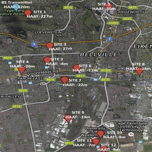
Figure 5 Measurement sites relative to BS transmitter.

5.4 Spectrum Measurements Setup

Outdoor spectrum measurements in the UHF frequency band were done at the chosen locations using a hand-held RF Explorer model WSUB1G, which has a measurement frequency range of 240 MHz to 960 MHz. The model was fitted with a Nagoya NA-773 wide band telescopic antenna with vertical polarization. The RF Explorer was connected to an Android phone running the RfTrack program [44] developed at ICTP that starts to measure spectrum immediately after the RF Explorer is connected using an On-The-Go (OTG) cable. Figure 6 shows a sample screen of the measurements from the RfTrack program. At each site, spectrum monitoring was done for 8 hours from 08:00 in the morning to 16:00 in the afternoon.

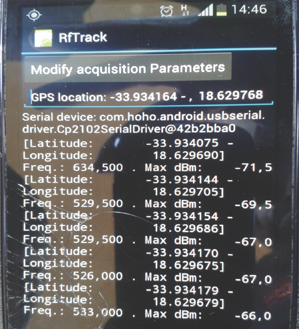
Figure 6 Android phone screen showing the measurement.

5.5 Results

The 8-hour measurements at each location in channel 22 from which the TV transmitter was broadcasting were averaged to establish the received signal power R_x. We used the average value of the measured power at the closest point to the BS transmitter (SITE 1) as a reference and estimate from there the power received at longer distances along the same approximate radial by using the Friis transmission equation [45] (Equation 7).

P r (d) = P r (d_{o}) + 20 * l o g (d_{o} / d) (7)

where Pr(d) is the received power at distance d in the same radial where d_o is calculated, Pr(d_o) is the received power at a close-in-reference-distance d_o.

In that way, we were able to compare the measurements with the values obtained using Equation 7. As Table 2 shows, there is reasonable agreement between the measured and calculated values. This confirm that the square law dependence of power loss with distance is adequate in this case since there are no obstacles in the trajectory. When obstacles are present, the factor multiplying the logarithm can be as high as 40 instead of 20.

Table 2 Comparison of calculated vs measured power

No.	Name	d_Km	Measured (dBm)	Calculate (Pr(d)) (dBm)	Measured – Calculated (dBm)
1	SITE 1	do = 0.54	Pr(d₀) = -80.39	Ref. power	-
2	SITE 2	2.37	-97.30	-93.24	-4.06
3	SITE 3	2.98	-86.45	-95.23	8.78
4	SITE 4	3.21	-93.34	-95.87	2.53
5	SITE 5	3.51	-94.52	-96.65	2.13
6	SITE 6	3.89	-92.58	-97.54	4.96
7	SITE 7	4.18	-96.43	-98.17	1.74
8	SITE 8	5.71	-97.75	-100.01	2.26
9	SITE 9	6.04	-91.77	-101.36	9.59
10	SITE 10	7.26	-97.33	-102.96	5.63
11	SITE 11	7.55	-94.25	-103.30	9.05
12	SITE 12	8.04	-94.23	-103.85	9.62

The value of the Effective Isotropic Radiated Power (EIRP) of the transmitter, the gain and return loss of a receiving antenna determine the real path loss. In this experiment, the transmitter antenna radiation pattern was unknown, which brings in a degree of uncertainty about the real EIRP of the transmitter in the direction where the measurements were made. Therefore, we had to make the following assumptions in order to be able to analyse the results further:

The published ERP of the TV transmitter (63.01 dBm) minus 2.15 dB is the EIRP in the direction where the measurements were taken and attribute the difference between the received power at the antenna input of the spectrum analyzer and the power read by the spectrum analyser at Site 1 as a resultant effect of the return loss and the antenna gain of the Nagoya NA-773 wide band telescopic antenna at the received frequency of 479.25 MHz of the TV transmitter.
The path loss at Site 1 (closest measurement point) from the TV transmitter is assumed to be equal to the free-space path loss at the corresponding 0.54 km distance (d_o). This value will be used to determine the received power at other distances by modifying the second term of Equation 7.

Assumption 1 is based on the fact that the square law dependence of power loss with distance is adequate and also that the measurements at similar distances from the TV transmitter are similar as shown in Table 2.

The effect of the return loss and the antenna gain of the Nagoya NA-773 telescopic antenna was regarded as a correction factor (CF) to every measurement. Using the FSPL Equation 8, the FSPL at 0.54 km distance and at the broadcasting frequency of 479.15 MHz was calculated as 80.71 dB, and the CF is then 60.54 dB (Assumed EIRP - measurement at Site 1 + assumed propagation loss at Site 1).

P_{L} = 32.45 + 20 * l o g (f) + 20 * l o g (d) (8)

where P_L is the free space path loss in dB, f is the frequency in MHz and d is the distance in kilometers.

The calculated CF was added to every measurement power at each location to get the corresponding antenna input power. Table 3 shows the measured power by the spectrum analyser at each measurement location and the corresponding spectrum analyser’s input power.

Table 3 Measured power and antenna input power

No.	Name	d_Km	Measured (dBm)	Antenna Input (dBm)
1	SITE 1	0.54	-80.39	-19.85
2	SITE 2	2.37	-97.30	-36.76
3	SITE 3	2.98	-86.45	-25.91
4	SITE 4	3.21	-93.34	-32.80
5	SITE 5	3.51	-94.52	-33.98
6	SITE 6	3.89	-92.58	-32.04
7	SITE 7	4.18	-96.43	-35.89
8	SITE 8	5.71	-97.75	-37.21
9	SITE 9	6.04	-91.77	-31.23
10	SITE 10	7.26	-97.33	-36.79
11	SITE 11	7.55	-94.25	-33.71
12	SITE 12	8.04	-94.23	-33.69

The path loss is calculated by subtracting the received signal at the antenna input at each measurement location from the EIRP (60.86 dBm). For each propagation model, the path loss from the TV transmitter is estimated for distances corresponding to those at which measurements were taken using their respective formulas. The path losses derived from the measurements and those estimated by the propagation models are shown in Table 4. To get a clearer picture of the losses predicted by the different models, they were plotted in the graphs shown in Figure 7. Path loss errors (average error, average absolute error, standard deviation, root mean square error (RMSE)) between measurements and the propagation models are shown in Table 5.

Table 4 Path losses

		Path Losses (dB)
Name	d_km	Measured	FSPL	L-R	F(50,50)	Ericsson 9999	Egli	Hata
SITE 1	0.54	80.71	80.71	99.70	54.33	90.68	86.32	108.88
SITE 2	2.37	97.62	93.56	97.10	68.19	110.18	112.01	131.17
SITE 3	2.98	86.77	95.55	99.50	68.19	110.18	115.99	134.62
SITE 4	3.21	93.66	96.19	95.40	71.46	114.18	117.28	135.75
SITE 5	3.51	94.84	96.97	99.70	72.39	115.36	118.84	137.09
SITE 6	3.89	92.90	97.86	98.80	73.52	116.72	120.62	138.64
SITE 7	4.18	96.75	98.48	99.60	74.32	117.66	121.87	139.73
SITE 8	5.71	98.07	101.19	109.70	77.90	121.78	127.29	144.43
SITE 9	6.04	92.09	101.68	102.30	78.62	122.52	128.27	145.27
SITE 10	7.26	97.65	103.28	105.50	81.19	124.94	131.46	148.05
SITE 11	7.55	94.57	103.62	104.70	81.77	125.46	132.14	148.64
SITE 12	8.04	94.55	104.17	105.40	82.70	126.29	133.23	149.58

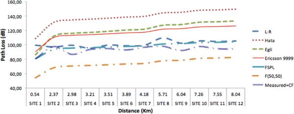
Figure 7 Plots of path losses.

5.6 Discussion of the Results

From the plots of the path losses in Figure 7 and the path loss errors in Table 5, the FSPL is the closest model to the measurements. This is not surprising since it is a consequence of the underlying assumptions made to derive the path loss from the measurements and due to the existence of a clear line of sight between the TV transmitter and the measurement locations. The L-R (ITM), calculated using Radio Mobile [37], was the closest fitting since it uses terrain elevation data over the trajectory to compute the path loss. From the figure and the table, the next model closest to the measurements was obtained from the F(50,50) curves although it consistently overestimated the received signal power (lower path losses). As a consequence of using the F(50,50), some available channels will be precluded for WSD use because they would be incorrectly flagged as occupied when in fact the received power is below the threshold. This is one of the failings of the F(50,50) curves, they over predict both coverage and interference distances particularly when used with the low resolution 30 arc-second terrain elevation database [46]. The Ericsson 9999, Egli and Hata models underestimated the received signal power since their path losses are greater than the path losses derived from the measurements done at each location, so their use in a geo-location database would not adequately protect primary users.

Table 5 Mean error, mean absolute error, standard deviation and RMSE

	Path Loss Errors (dB)
Name	Measured & FSPL	Measured & L-R	Measured & F(50,50)	Measured &Ericssion 9999	Measured & Egli	Measured & Hata
SITE 1	0.00	18.99	-26.38	9.98	5.61	28.17
SITE 2	-4.06	-0.52	-29.43	12.56	14.40	33.55
SITE 3	8.78	12.73	-16.10	26.43	29.22	47.86
SITE 4	2.53	1.74	-22.20	20.52	23.63	42.09
SITE 5	2.13	4.86	-22.45	20.52	24.00	42.25
SITE 6	4.96	5.90	-19.38	23.82	27.72	45.74
SITE 7	1.74	2.85	-22.43	20.91	25.12	42.98
SITE 8	3.12	11.63	-20.17	23.71	29.22	46.36
SITE 9	9.59	10.21	-13.47	30.43	36.18	53.18
SITE 10	5.63	7.85	-16.46	27.29	33.81	50.40
SITE 11	9.05	10.13	-12.80	30.89	37.57	54.07
SITE 12	9.62	10.85	-11.85	31.74	38.69	55.04
Mean	4.42	8.10	-19.43	23.23	27.10	45.14
Mean absolute	5.10	8.19	19.43	23.23	27.10	45.14
Standard deviation	4.32	5.45	5.49	6.87	9.67	8.11
RMSE	6.06	9.64	20.12	24.15	28.64	45.80

Although the FSPL model is closest to the measurement data as its RMSE (6.06 dB) from Table 5 falls within the acceptable range of 6–7 dB for urban areas [47], we cannot extrapolate this results to other types of terrain different from the one used in this work. Extensive long-hours spectral measurements are needed and also more measurement sites need to be included to confirm the validity of a model for the area, which may be costly and time consuming.

6 Experimental Bench-Marking

Related experiments have been conducted in other regions of the world. A comparison is made between those experiments and our experiment in terms of equipment used and the results obtained.

Commercial high-end spectrum analyzers for monitoring the RF spectrum are expensive (in the order of many thousand dollars) and are not typically available in university laboratory of most developing countries [48].

However, affordable off-the-shelf RF spectrum analyzers are becoming available, making them more attractive to the developing world. A random sample of the literature covering experiments to measure path losses shows that low-cost, portable and easy-to-use spectrum analyzers are being preferred over the expensive and bulky commercial high-end spectrum analyzers. Table 6 shows some of the surveyed experiments. In the table, all except two experiments, [49] and [50], used a variation of the low-cost, easy-to-use, portable RF spectrum analyzer. In [49], the commercial high-end spectrum analyzer was used while in [50], the type of RF spectrum analyzer used was not mentioned. The preference for easy-to-use and low-cost RF spectrum analyzers confirms their adequacy for spectrum occupancy measurements.

Table 6 Experiments bench-marking

Country	Location Classification	Spectrum Analyzer	Best-Fit Model	RMSE for Best-Fit Model (dBm)
Greece [51]	urban	Rohde & Schwarz FSH-3	Longley-Rice ITM	3.60
Brazil [49]	urban	ANRITSU MS8901A	ITU-RP.1546	11.29
Nigeria [52]	urban, suburban, rural	N9342C Agilent	None	-
Namibia [50]	urban	unknown	Ericsson	3.73
Malawi [53]	Semi-urban	Handheld Spetrum Analyzer	SPM	-
South Africa (our experiment)	urban	RF-Explorer	FSPL	6.06

Different best-fit propagation models were found by the experiments. This is in agreement with the finding that propagation models are environment and area dependent. The FCCs recommended terrain-based modeling such as the Longley-Rice propagation methodology performed well in experiment [51] with an RMSE of 3.60 dB. In [49], ITU-R P.1546 was found to be the best-fit model with RMSE of 11.29 dB in three of the five cities where the experiment was carried out. In [52], no single model was found that produced a good fit consistently in all the areas experimented. In [50], Ericsson propagation model was the best-fit model with RMSE of 3.73 dB after a correction factor was added to the models equation. In [53], Standard Propagation Model (SPM) in the Asset network planning tool fitted well with the measurements.

Experiments performed in different environments found dissimilar best-fitted propagation models. This clearly shows that propagation models cannot be extrapolated from one area to another. The best way to assess the fitness of a model in an area is by carrying out RF spectrum measurement and compare the results with those predicted by a given model.

7 Conclusion

Discussions in the literature, mostly based on the developed world environment, have placed much emphasis on the limitations of the spectrum sensing approach while ignoring the limitations of the geo-location database approach when applied in the developing world. This paper considered a broader analysis of the situation by looking at factors that can affect the performance of each approach and how these factors can affect their applicability in developing regions. In so doing, the paper has highlighted the need to conduct more research on the performance of spectrum sensing in regions where plenty of white spaces are available, e.g., rural areas of developing world countries.

Our analysis concludes that information that is needed by the geo-location database approach to perform optimally may not exist in most developing world countries, especially in the rural areas where telecommunication infrastructure is lacking and white spaces are abundant. Based on the absence of factors required by the geo-location approach to perform optimally, and considering the implementation, maintenance and administrative cost of geo-location approach, we have concluded that spectrum sensing is a better approach to use in rural areas of developing world countries. However, further investigations of (i) the management of white spaces to support their efficient trading between their primary and secondary users and (ii) propagation characteristics of their waves when used for outdoor deployments [54] are needed to support their wide-scale deployment in the regions of the developing world. These investigations are a potential avenue for future work.

References

[1] Barnes, S. D., Van Vuuren, P. J., and Maharaj, B. T. (2013). “Spectrum occupancy investigation: measurements in South Africa.” Measurement, 46(9), 3098–3112.

[2] FCC, U. S., and Docket, E. T. (2008). “Second Report and Order and Memorandum Opinion and Order, in the Matter of Unlicensed Operation in the TV Broadcast Bands Additional Spectrum for Unlicensed Devices below 900 MHz and in the 3 GHz band.” Washington, DC: Federal Communnications Commission.

[3] Garrido, H. A. A., Rivero-Angeles, M. E., and Flores, I. Y. O. (2016). “Performance analysis of a wireless sensor network for seism reporting in an overlay cognitive radio system,” in Proceedings of the Advanced Information Networking and Applications Workshops (WAINA), 30th International Conference on. IEEE, Rome.

[4] Naik, G., Singhal, S., Kumar, A., and Karandikar, A. (2014). “Quantitative assessment of TV white space in India,” in Proceedings of the Twentieth National Conference on Communications (NCC), Kanpur, 16.

[5] Akyildiz, I. F., Lee, W., Vuran, M. C., and Mohanty, S. (2006). “Next generation/dynamic spectrum access/cognitive radio wireless networks: a survey.” Comput. Netw. 50:2127–2159.

[6] Kaniezhil, R., and Chandrasekar, C. (2012). “Performance evaluation of qos parameters in dynamic spectrum sharing for heterogeneous wireless communication networks.” Int. J. Comput. Sci. 9, 81–87.

[7] Yuan, Y., Bahl, P., Chandra, R. T., Moscibroda, R., and Wu, Y. (2007). “Allocating dynamic timespectrum blocks in cognitive radio networks,” in Proceedings of the 8th ACM International Symposium on Mobile ad Hoc NetWorking and Computing, New York, NY.

[8] Carlson, J., Ntlatlapa, N., King, J., Mgwili-Sibanda, F., Hart, H., Geerdts, C., et al. (2013). “Studies on the use of television white spaces in south africa: recommendations and learnings from the cape town television white space trial.” Available at: https://www.tenet.ac.za/tvws/recommendation-and-learnings-from-the-cape-town-tv-white-spaces-trial

[9] Masinde, M., and Bagula, A. (2010). “A framework for predicting droughts in developing countries using sensor networks and mobile phones,” in Proceedings of the 2010 Annual Research Conference of the South African Institute of Computer Scientists and Information Technologists (SAICSIT 2010). New York, NY, 390–393.

[10] Masinde, M., Bagula, A., and Nzioka Mthama, T. (2012). “The role of ICTs in down-scaling and upscaling integrated weather forecasts for farmers in sub-Saharan Africa,” in Proceedings of the ICTD12. New York, NY: ACM, 122–129.

[11] Mandava, M., Lubamba, C., Ismail, A., Bagula, H., and Bagula, A. (2016). “Cyber-healthcare for public healthcare in the developing world,” in Proceedings of the 2016 IEEE Symposium on Computers and Communication (ISCC 2016) Rome, 14–19.

[12] Bagula, A., Lubamba, C., Mandava, M., Ismail, A., Bagula, H., Zennaro, M., and Piet-rosemoli, E. (2016). “Cloud based patient prioritization as service in public health care,” in Proceedings of the ITU Kaleidoscope, Bangkok, 14–16.

[13] Bagula, A., Castelli, L., and Zennaro, M. (2015). “On the design of smart parking networks in the smart cities: An optimal sensor placement model.” Sensors 15, 7.

[14] Brown, T., Pietrosemoli, E., Zennaro, M., Bagula, A., Mauwa, H., and Nleya, S. A. (2014). “Survey of TV White Space Measurements,” in e-Infrastructure and e-Services for Developing Countries. Berlin: Springer International Publishing, 164172.

[15] Mancuso, A., Probasco, S., and Patil, B. (2013). “Protocol to Access White-Space (paws) Databases: Use Cases and Requirements.” Technical Report, Internet Engineering Task Force 2013.

[16] Murty, R., Chandra, R., Moscibroda, T., and Bahl, P. (2012). “Senseless: a database-driven white spaces network.” IEEE Trans. Mobile Comput. 11:189203.

[17] Zurutuza, N. (2011). “Cognitive radio and tv white space communications: Tv white space geolocation database system.” Trondheim: Norwegian University of Science and Technology.

[18] ECC CEPT. (2011). “Technical and operational requirements for the possible operation of cognitive radio systems in the white spaces of the frequency band 470–790 MHz.” ECC Rep. 159, 2011.

[19] Hoven, N., and Sahai, A. (2005). “Power scaling for cognitive radio,” in Proceedings of the International Conference on Wireless Networks, Communications and Mobile Computing, Maui, 1:250–255.

[20] Ruttik, K. (2011). “Secondary spectrum usage in tv white space.” Doctoral dissertations, Espoo.

[21] Okumura, Y., Ohmori, E., Kawano, T., and Fukuda, K. (1968). “Field strength and its variability in VHF and UHF land mobile radio service.” Rev. Elec. Commun. Lab, 16:82–573.

[22] Hata, M. (1980). “Empirical formula for propagation loss in land mobile radio services.” Vehicular Technol. IEEE Trans. 29:317–325.

[23] Yin, Y., Wu, K., Yin, S., Li, J., Li, S., and Ni, L. M. (2012). “Digital dividend capacity in China: A developing countrys case study,” in Proceedings of the IEEE International Symposium on Dynamic Spectrum Access Networks (DYSPAN), Rome, 121–130.

[24] Damosso, E., and Correia, L. M. (1991). “Urban transmission loss models for mobile radio in the 900 and 1,800 MHz bands.” Hague: COST.

[25] Milanovic, J., Rimac-Drlje, S. and Majerski, I. (2010). “Radio wave propagation mechanisms and empirical models for fixed wireless access systems.” Technical Gazette 17:43–52.

[26] Yucek, T., and Arslan, H. (2010). “A survey of spectrum sensing algorithms for cognitive radio applications,” in Proceedings of the Communications Surveys & Tutorials, IEEE, Rome, 11.

[27] Zhang, T., Leng, N., and Banerjee, S. (2014). “A vehicle-based measurement framework for enhancing whites-pace spectrum databases,” in Proceedings of the 20th annual International Conference on Mobile Computing and Networking, New York: ACM, 17–28.

[28] Mishra, S. M., and Sahai, A. (2010). “How much white space has the FCC opened up,” in Proceedings of the IEEE Communication Letters, Rome.

[29] Mancuso, A., Probasco, S., and Patil, B. (2013). “Protocol to Access White-Space (paws) Databases: Use Cases and Requirements.” Technical report Internet Engineering Task Force.

[30] WG802.11 Wireless LAN Working Group. “802.11af – IEEE standard for information technology – telecommunications and information exchange between systems – local and metropolitan area networks.” Electronic, IEEE Standards Association. Available at: http://standards.ieee.org/getieee802/download/802.11af-2013.pdf, 2013.

[31] Federal Communications Commission et al. (2010). “Second Memorandum Opinion and Order in the Matter of Unlicensed Operation in the TV Broadcast Bands and Additional Spectrum for Unlicensed Devices Below 900 MHz and in the 3 GHz Band.” Washington, DC: Federal Communications Commission.

[32] Gonçalves, V., and Pollin, S. “The value of sensing for TV white spaces,” in Proceedings of the IEEE Symposium on New Frontiers in Dynamic Spectrum Access Networks (DySPAN), Rome.

[33] Pietrosemoli, E., and Zennaro, M. (2013). “TV white spaces. A Pragmatic Approach,” 1:35–40.

[34] Federal Communications Commission. (1998). “Advanced Television Systems and Their Impact upon the Existing Television Broadcast Service.” Washington, DC: Federal Communications Commission.

[35] Ruck, J. D. (2017). “Fundamentals of AM, FM, and TV Coverage and Interference Considerations.” Markley, D. L. & Associates, Inc. Available at: http://www.sbe24.org/wba-sbe-shows/archives/Clinic2008/Ruck-Ma rkley-2008.pdf. [accessed January, 27 2017].

[36] Seybold, J. S. (2005). “Introduction to RF Propagation.” Berlin: John Wiley & Sons.

[37] Coude, R. (2016). “Radio Mobile RF propagation simulation software.” Available at: http://radiomobile.pe1mew.nl/, 1988, [accessed May, 12 2016].

[38] Oluwole, F. J., Olajide, O. Y. (2013). “Radio frequency propagation mechanisms and empirical models for hilly areas.” Int. J. Elect. Comput. Eng. 3:372–376.

[39] Wang, H., Noh, G., Kim, D., Kim, S., and Hong, D. (2010). “Advanced sensing techniques of energy detection in cognitive radios.” J. Commun. Netw. 12:19–29.

[40] Chebil, J., Lawas, A. K., and Islam, M. D. (2013). “Comparison between measured and predicted path loss for mobile communication in malaysia.” World Appl. Sci. J. 21:123–128.

[41] Shabbir, N., Sadiq, M. T., Kashif, H., and Ullah, R. (2011). “Comparison of radio propagation models for long term evolution (LTE) network.” Int. J. Next Gen. Netw. 3:2–7.

[42] ICASA. (2013). “Terrestrial Broadcasting Frequency Plan.” Independent Communications Authority of South Africa (ICASA).

[43] Federal Communications Commission (FCC). (2016). “Antenna Height Above Average Terrain (HAAT) Calculator.” Available at: https://www.fcc.gov/media/radio/haat-calculator [accessed July, 3 2016].

[44] Rainone, M., Zennaro, M., and Pietrosemoli, E. (2016). “RFTrack: a tool for efficient spectrum usage advocacy in Developing Countries,” in Proceedings of ICTD 2016, Ann Arbor, 36.

[45] Rao, S. (2007). “Estimating the zigbee transmission-range ism band-designers of short-range wireless devices in the 900-MHz and 2.4-GHz band need to understand what and how parameters affect the transmission range.” EDN 52:67–74.

[46] Vernier. D. (2012). “Broadcast Propagation Prediction Methodology: Knowing Where your Signal Goes.” Available at: http://www.v-soft.com/wp-content/uploads/2012/04/Propagation.pdf, 2012, [accessed February, 19 2017].

[47] Blaunstein, N., Censor, D., Katz, D., Freedman, A., and Matityahu, I. (2003). “Radio propagation in rural residential areas with vegetation.” Prog. Electromagnet. Res. 40:131–153.

[48] Zennaro, M., Pietrosemoli, E., Mlatho, J. S. P., Thodi, M., and Mikeka, C. (2013). “An assessment study on white spaces in Malawi using affordable tools,” in Proceedings of the Global Humanitarian Technology Conference (GHTC), Rome, 265–269.

[49] Silva, F. S., Matos, L. J., Peres, F. A. C., and Siqueira, G. L. (2013). “Coverage prediction models fitted to the signal measurements of digital tv in brazilian cities,” in Proceedings of the Microwave & Optoelectronics Conference (IMOC), 2013 SBMO/IEEE MTT-S International. IEEE, Porto de Galinhas, 1–5.

[50] Temaneh-Nyah, C., and Nepembe, J. (2014). “Determination of a suitable correction factor to a radio propagation model for cellular wireless network analysis,” in Proceedings of the Intelligent Systems, Modelling and Simulation (ISMS), 2014 5th International Conference on. IEEE, Langkawi, 175–182.

[51] Kasampalis, S., Lazaridis, P. I., Zaharis, Z. D., A. Bizopoulos, Zettas, S., and Cosmas. J. (2014). “Comparison of longley-rice, itu-r p. 1546 and hata-davidson propagation models for dvbt coverage prediction.” BMSB, 2014:1–4.

[52] Faruk, N., Ayeni, A., and Adediran, Y. A.(2013). “On the study of empirical path loss models for accurate prediction of tv signal for secondary users.” Prog. Electromagnet. Res. 49:155–176.

[53] Mikeka, C., Thodi, M., Mlatho, J. S. P., Pinifolo, J., Kondwani, D., Momba, L., Zen-naro, M., and Moret, A. (2014). “Malawi television white spaces (tvws) pilot network performance analysis.” J. Wireless Netw. Commun. 4:26–32.

[54] Zennaro, M., Ntareme, H., and Bagula, A. (2008). “Experimental evaluation of temporal and energy characteristics of an outdoor sensor network,” in Proceedings of the International Conference on Mobile Technology, Applications, and Systems, New York, NY: ACM.

Biographies

H. Mauwa received his M.Sc. degree in Information Technology in 2007 from Nelson Mandela Metropolitan University (NMMU) in South Africa and is presently studying towards his Ph.D. in Computer Science at the University of the Western Cape (UWC) also in South Africa. His Ph.D. research focuses on methods for accessing TV white spaces in developing countries.

A. Bagula obtained his doctoral degree in 2006 from the KTH-Royal Institute of Technology in Sweden. He held lecturing positions at Stellenbosch University (SUN) and the University of Cape Town (UCT) before joining the Computer Science department at the University of the Western Cape in January 2014. Since 2006, He has been a consultant of UNESCO, the World Bank and other international organizations on different telecommunication projects. His research interest lies on the Internet-of-Things, Big Data and Cloud Computing, Network security and Network protocols for wireless, wired and hybrid networks.

M. Zennaro received his M.Sc. degree in Electronic Engineering from University of Trieste in Italy. He defended his Ph.D. thesis on Wireless Sensor Networks for Development: Potentials and Open Issues at KTH-Royal Institute of Technology, Stockholm, Sweden. His research interest is in ICT4D, the use of ICT for development. In particular, he is interested in Wireless Networks and in Wireless Sensor Networks in developing countries. He has been giving lectures on Wireless technologies in more than 20 countries.

E. Pietrosemoli is a researcher at the Telecommunications and ICT for Development Lab of the International Centre for Theoretical Physics in Trieste, Italy, and president of Escuela Latinoamericana de Redes. He holds an MSc. degree in Electrical Engineering from Stanford University. After teaching telecommunications for 30 years at Universidad de los Andes in Venezuela, he is currently focused on means to provide low cost long distance wireless data communications.

A. Lysko has a Ph.D. in Information and Communication Technologies (ICT) from the Norwegian University of Science and Technology (NTNU), Norway. He has worked in industry and at universities, and is presently a Principal Researcher with the Council for Scientific and Industrial Research (CSIR). Dr. Lysko has 2 patents and several patent applications, published over 50 research papers and popular articles as well as a book and 2 book chapters.

T. X. Brown is a Professor in Electrical, Computer, and Energy Engineering and served as Director of the Interdisciplinary Telecommunications Program at the University of Colorado, Boulder. He received his B.S. in physics from Pennsylvania State University and his Ph.D. in electrical engineering from California Institute of Technology in 1990. His research interests include adaptive network control, machine learning, and wireless communication systems.