Energy Efficient Data Gathering by Using Optimum Pattern Recognition with Relocalization in Mobile Wireless Sensor Networks

S. Sivasakthiselvan¹ and V. Nagarajan²

Research Scholar¹, Professor & Head²

Department of Electronics and Communication Engineering, Adhiparasakthi Engineering College, Melmaruvathur 603319, Tamil Nadu, India

E-mail: mangaivasan@gmail.com

Received 26 July 2017;
Accepted 18 January 2018

Abstract

The Efficient Localization and Data Gathering in Mobile wireless sensor networks (MWSNs) is considered as an evolving technology for many system applications like military surveillance, health monitoring and reporting to ambulance team, tracking the animal migration patterns, etc.,. The wireless sensor nodes with the ability to report the location information and sensory data. Therefore, there have been a numerous significances on localization and Energy Efficient data gathering in MWSNs in the past few years. In this paper, our proposed system Energy Efficient Data Gathering Pattern (EEDGP) is performs in two phases. In the first phase the recognition of pattern is done by K-Means technique. The K-Mean clustering is simple and understandable algorithm based on the attributes and it is used to generate the specific number of disjoint clusters. Also the maximum distance which travels by the node and velocity of the node is estimated by Hop count measurement Markov Decision Process (MDR) is proposed to check the inaccuracy of localization. In the second phase global relocalization is carried out based on the result of the local relocalization and it performs global time synchronization for data gathering from the Mobile Agent (MA) in the network. We compared our proposed algorithm with other approaches in Network lifetime, Energy consumption, Packet delivery ratio, and Time Complexity. The simulation results proved the effectiveness of the proposed algorithm over similar methods.

Keywords

• Mobile Wireless Sensor Networks
• Efficient Data Gathering System (EDGS)
• Local Relocalization & Global Relocalization
• Time Bound Essential Localization (TBEL)
• Hop-Distance Estimation and Backoff-Based Message Broadcast

1 Introduction

Wireless sensor network is a combination of millimeter-scale, self-contained, micro-electro mechanical devices [1]. These devices generally posses sensors, CPU power, wireless transmitter and the receiver and the power supply. WSN’s are intelligent and designed to use processing of in-network. In many application areas, large number of sensor nodes are used, here, [2] we use clustering architecture where a wide number of sensors are deployed for monitoring purpose. Localization is widely used in WSN to identify the current location of the sensor nodes. When a node moves across the specific area, the neighboring node predicts the node movements and target entrance to another area [1]. Though it provides the advantages of localization in advance it also provides an issue of repeated localizing the mobile nodes. To overcome this obstacles relocalization concept is implemented in this paper. Since the node’s are in movement, we must relocalize the time bound and update localization information. The relocalization of the entire network is done either locally or globally in the predefined time intervals. In this paper TBR methodology is implemented in order to determine the optimum time to trigger the relocalization. The proposed algorithm is divided into two steps: local relocalization and global relocalization. This algorithm will extensively reduce the localization error. In the first step analysis of clustering is done by pattern recognition concept. The objective of pattern recognition is to assign the object or event to one of the number of categories based on features derived. Generally, pattern recognition consists of three steps unsupervised learning, supervised learning and semi supervised learning. The unsupervised learning is a basic task to classify the labels. This learning is again subdivided into two groups, clustering and blind signal separation.

2 Related Works

There are different localization algorithms present. Here, the time bounded localization algorithm is closely related to our proposed model. The Time bounded essential localization (TBEL) algorithm which is helpful for localizing a sensor node within a predefined time [3]. The need for TBEL is, the localization must be completed within a short duration when the node is on the time critical path and generally localization process requires exchange of messages between the sensor nodes within a particular time in order to find the position of the neighboring nodes. In TBEL, the node localization is done by forming a local coordination system (LCS) with its closest neighboring nodes. When comes to global localization, three nodes are represented as anchor nodes in each LCS in order to perform the local localization. For doing this, the anchor nodes should be aware of its position. It finds its position by GPS. Then the nodes repeatedly broadcast signals [4]. The usage of TBEL algorithm leads to presence of localization. So we go for Time bounded Relocalization (TBR) algorithm in our work.

Hierarchical clustering algorithm which comes under unsupervised learning type in pattern recognition. It is no need for pre-specification of number of clusters [2]. There are two different types in hierarchical clustering. They are agglomerative clustering and divisive clustering. Agglomerative clustering is one of the bottom up approaches with a number of singleton cluster in which each cluster has sub clusters. The drawback of this agglomerative clustering is, that the objects are initially localized, incorrectly so they can be relocated later and distance metrics can vary the results. Another one is divisive clustering, which is one of the top down approach. This is similar to the type agglomerative clustering, but divisive clustering works in the opposite direction [5]. Initially in this a single cluster contains all the objects and splitting of that cluster takes place until single objects remains in a single cluster. The drawback of divisive clustering is splitting up of clusters leads to computational difficulties and there is a variation in results based on the usage of different distance metrics. This clustering algorithm is used in mathematical chemistry and petroleum geology. The major drawback in overall hierarchical clustering is its slow run time. But K-mean clustering has a faster run time when compared to hierarchical clustering. So we use K-mean clustering in our proposed model.

2.1 Time Bound Essential Localization (TBEL)

TBEL algorithm is proposed in the situation that require the specific time for localization such as in military areas, in order to avoid the attacks, location of node’s should be determined in a limited time interval [6].

In TBEL, two steps are involved in the localization process such as essential and global localization initially K several LCS’s are formed during communication rounds which are called essential localization. Then the global localization occurs through communications between the LCS’s that have been formed during essential localization. Message flooding carried out continuously until all LCS’s are formed and thus network get essentially localized, then communication between LCS’s results in global localization. After multiple flooding if some LCS’s do not attach with other LCS’s, then they will remain unlocalized, which is called isolated islands. In such places, the isolated islands can be attached with fixed anchor nodes in staticnetworks.

However to apply TBEL algorithm, the relative movement of the sensor need to be re-localized at a certain time bound and frequently update the localization information. At the proper time interval either locally or globally the re-localization of the entire network is under one technique. After an extensive time period if relocalization happens, the precision of location estimation will be degraded. Contra wise, if same process repeats and performs constantly in shorter periods, higher expenses will be forced upon thesystem [7–10].

The objective is to progress an efficient re-localization algorithm to identify the optimum relocalization time with minimum localization error in WSN. Towards this objective, modified TBEL (TBL) algorithm is proposed, where the mobility of sensor is included to gain the best time to startrelocalization.

2.2 Time Bound Localization (TBL)

In this algorithm, the sensor nodes are localized within a specific time bound. In TBR algorithm the relocalization process is carried out in many rounds of message flooding and it is limited to a specific K value. At single round of message flooding a node transmits and receives data from all neighbouring nodes. The time required to localize the network is determined based on the number of communication rounds [8]. Within a K round of communication all sensor nodes in K-hop can be localized at a particular value of K, but anchor nodes present away K-hops and cannot contribute to localization of specific nodes. If the two particular nodes have the greatest distance, then the number of hops to connect the nodes can be estimated as an upper bound for K. This upper bound depends on the node’s transmission range. The coordination of each node is determined by the communication between neighboring nodes. The location estimation methods like trilateration and multilaterations are used to estimate the distance between the nodes and calculate their locations. After the K-rounds of message flooding, the complete networks are localized globally. Since, the anchor nodes know their locations in the global coordinate system, it will result in global localization [9–15]. Generally, large number of anchor nodes can be localized but in practice only a small number of anchors are used due to the high cost of the algorithm. In this algorithm, it is assumed that at initial round the anchor node broadcast messages like their locations while, the unlocalized mode gains signal from at least three anchor nodes, can estimate their distances to anchor which uses the three circle intersection formulas for their locationestimation [10–18].

In the next rounds of communication, the newly localized nodes will also broadcast their locations which help the rest of unlocalized nodes. This process repeats continuously for predefined k rounds. After K rounds the nodes stops sending signals, but some nodes still do not connect to at least three anchor nodes. Since, the major objectives are to identify the optimum time to trigger the relocalization, the accuracy of location estimation is degraded. Based on the analysis, Time Bound Relocalization (TBR) algorithm is proposed to estimate the optimum relocalization time, which will reduce the localization error in minimum [19, 20].

2.3 Efficient Data Gathering System (EDGS)

More recently, the Efficient Data Gathering System (EDGS). It uses a random walk manner to estimate the next position of the data collection. To determine the optimal data transmission path, a relay point selection is used. The transmission data will be passed through the relay point by the sink to the data collector. EDGS mainly focus for improving the triangular routing problem and decrease the signaling overhead. It only considers the distance to the mobile collector for intermediate node selection mechanism. The mobility angle and speed of the mobile data collector does not consider while data collection process. So, this could lead to routing the data through a longer path, introducing considerable delays on data delivery and bandwidth wastage. Furthermore, the relay node selection mechanism does not take into account the residual energy of the relay node, which cause result in network segmentation, and unbalanced energy within the network nodes.

3 Proposed System

3.1 System Overview

The proposed method consists of two step relocalization procedure. In general localization, each node knows their position within their communication range for the entire area. Relocalization can be estimated at every pre-defined time interval. If the speed of the nodes differs, then relocalization can be done at different time interval. However, its complexity and time consumption increases to perform the individual relocalization [9]. In order to overcome this problem, the whole network is divided into several clusters and each cluster is relocalized at a specific time depending on the average speed of nodes belonging to the corresponding cluster. This process is known as the Local Relocalization (step-1). Thus, the optimum time to trigger relocalization can be estimated. In order to achieve this, it is necessary to identify the maximum distance travel by each node and its velocity in each isolated cluster. With the result of local relocalization, global relocalization, data gathering and control can be performed as step-2.

3.1.1 Localization of nodes

Localization is one of the important concepts used in wireless sensor networks. It is used to find the current location of the sensor nodes. In order to find the location of the nodes, we generally install GPS on each node. It leads to be more expensive and also it is difficult to get the exact location in indoor environments. Manual configuration of location is also difficult for dense network. So, in order to find the current position of the sensor node without manual configuration and hardware, we go to the concept called localization where the exact location of the sensor nodes is easilydetermined [16].

The localization technique can be classified into two types, that is range-free scheme and range based method. In range based method, the range of the sensor node information is used to calculate the distance between each node. Here the localization can be carried out with or without the anchor nodes. In rage free methodology, they do not require special hardware for finding the location process. Here the sensor node location and their distance compute by DV distance or DV Hop-count. It is also carried with or without anchor nodes. Thus, each localization technique serves different purposes. However, when we use more number of anchor nodes that favors less the localization errors.

3.1.2 Cluster formation of nodes

After localizing the nodes, we need to form the cluster. Clustering is essential for sensor network application where a large number of ad hoc sensors are deployed for sensing purposes. Generally, the strategy of clustering is teaming up nodes in virtual groups with one head per group. Clustering techniques are diverse but a common is based on converting flat network into a clustered network by assigning roles such as cluster head, cluster member and gateway. The cluster formation process requires the transmission of controlled information. The node transmits in such a node identity, list of neighbors, mobility, battery level etc., this information is required for cluster head selection and cluster formation process. Disturbances can occur due to node mobility, battery limitation, lack of coverage, etc., So, there is a need for maintenance of the cluster. It involves three different approaches for cluster maintenance such as continuous, event-driven or temporized. Then, the anchor important task in clustering is a cluster head role assignment.

3.1.3 Pattern recognition of cluster

After the formation of clusters, there is a need for identifying its pattern. A pattern is generally an entity like a human face, handwritten word or fingerprint image that could be given a name. Recognition is an act of associating a classification with a label. Pattern recognition is the science of making inferences based on data. Its objective is to assign an object or event a number of categories based on features derived to emphasize commonalities. Pattern recognition generally involves three types of learning, unsupervised learning, supervised learning and semi supervised learning.

The process of pattern recognition is the signal which is post processed, i.e. they are filtered to reduce the inefficient path selection and maximize the location accuracy. Then it is completes the optimal amount of needed information. Finally, classification takes place to map a sensed event described by the feature vector to a recognized class by a classifier. There are several algorithms used for pattern recognition. Some of the algorithms involve the concept of both localization and clustering. The Figure 1 shows the different pattern recognition with clustering are K-mean clustering, hierarchical clustering and the algorithms with localization are stochastic pattern recognition. The S₁, S₂, S₃ is active sensor nodes, M₁, M₂, M₃, M₄ is the Cluster Head or Mobile Agents (MA).

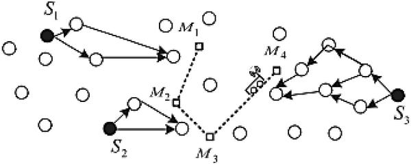
Figure 1 Pattern recognition.

3.1.4 Relocalization of nodes

After performing the pattern recognition of clusters, there might be changes in the location of sensors due to the mobile nodes. It leads to some localization error. So, we need to perform the relocalization process. Relocalization is nothing but retrigger the nodes with an optimum time interval. There are two types of relocalization. One is local relocalization and another one is global relocalization. In local relocalization, the nodes in the particular island is relocalized. Thus, the relocalization reduces the localizationerror.

3.1.5 Global relocalization and data gathering

In global relocalization, the nodes are relocalized with the estimated value from the local relocalization and gathering datas from various mobile agents or cluster heads through the mobile unit.

3.2 Sequence Diagram

In this section Figure 2, Sequence diagram is proposed to calculate the optimum time to trigger relocalization. The proposed sequence is also validated using the result of mathematical analysis of cluster formationin Figure 4.

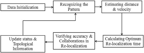
Figure 2 Sequence diagram of EEDGP.

The algorithm analysis of clustering is done by pattern recognition, which is the science of making inferences based on data.. The objective of pattern recognition is to assign the object or event to one of the number of categories based on features derived. Generally, pattern recognition consists of three types of learning. They are supervised learning, machine learning and unsupervised learning. Cluster based pattern recognition is done by unsupervised learning that is K mean in this paper. Based on the attribute, K mean algorithm are used to generate specific number of disjoint and non-hierarchical clustering. The Figure 3 shows To find the cluster, it is said to be iterative and non-deterministic method. Thus k-mean results in minimizing the intra cluster distances and inter cluster distance are maximizedin clustering.

3.2.1 K-Mean implementation

Figure 3 K-mean Implementation.

Procedure 1: Consider K points to be clustered X₁,…, X_K. These K point are being represented in the space in which objects are clustered. Thus, initial centroid is represented by these points.

Procedure 2: Each and every object formed as a group that has closest centroid.

$$\text{M}K=\frac{{\displaystyle {\sum }_{i:Cu(i)=k^{Xi}}}}{N_k}\left(1\right)$$

Where, k=1,2,3,…, K.

• Cu(i) is the number of clusters
• Mk is mean vector of K^th cluster.
• N_k is number of observations in cluster.

Procedure 3: Once all objects are assigned in the group, the position of the K-centroid are recalculated.

$$Cu(i)={\text{argmin}}_{\text{1}\le \text{k}\le \text{K}}^{\parallel \text{}\text{}\text{Xi-M}k\text{}\text{}{\parallel }^{\text{2}}},\text{i}=1,2,\dots ,\text{N}\left(2\right)$$

Procedure 4: 2 and 3 are repeated until no other possible distinguished centroid is found.

$$\begin{array}{ll}E\left(Cu\right)\hfill & =\frac{1}{2}{\displaystyle \sum _{k=1}^K{\displaystyle \sum _{Cu\left(i\right)=k}{\displaystyle \sum _{Cu\left(j\right)=k}\parallel \text{}\text{}Xi-Xj\text{}\text{}{\parallel }^2}}\left(3\right)}\hfill \\ \hfill & ={\displaystyle \sum _{k=1}^{K}N\text{k}{\displaystyle \sum _{Cu\left(\text{i}\right)}\parallel \text{}\text{}\text{Xi-m}k\text{}\text{}{\parallel }^{\text{2}}\left(4\right)}}\hfill \end{array}$$

Procedure 5: Thus intra cluster distances are minimized and inter cluster distance is maximized in clustering.

After identifying the pattern the relocalization triggering time is estimated in two steps which are explained as follows.

3.2.2 Local relocalization

The maximum distance travel and maximum average node velocity v are identified for local relocalization from the velocity of the node and the dimension of the area. Each clusters in the network (island) is relocalized time T_local. Thus T_min and T_max are calculated followed by the hop distance measurement.

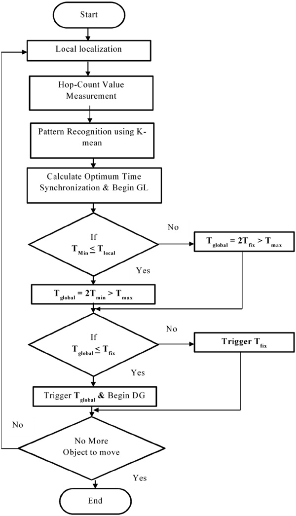
Figure 4 Execution of EEDGP.

3.2.3 Hop-count value measurement and back off-based message broadcast

Within the first step, every anchor node publicizes a beacon message for the duration of the network. Those beacon messages consist of the anchor’s region and a hop count number zero in the beginning stage. Every receiving node sustains a minimum in line with-anchor hop count number based totally on all received beacon messages. When the received beacon message count is greater than the given anchor nodes, they are overlooked and get rejected. However, when the hop count is increased the legitimate beacon messages are forwarded to other regular nodes. Through this, all nodes within the link can discover their minimum hop counts to each anchor node. On the other hand, this modest flooding method outcomes in immoderate message overhead. To Overcome the computational complexity, we go for a back-off based broadcasting mechanism.

The conventional hop-be counted localization strategies require two separate flooding ranges: (a) hop value accumulation and (b) calculation of average-hop distance. Every anchor node measures a current hop space during the flooding structure based totally on the hop counts from other anchors. Upon getting a beacon signal, a node will increase the hop value. If the new hop value is larger than the saved minimal hop value, the beacon signal will be rejected. If the new hop value is less than the stored minimum hop value, it will reorganize and forward the respective beacon signal. In a network, active node can additionally receive numerous beacon signals about the equal anchor and that can be guide a smaller hop values among the network nodes.

3.2.4 Global relocalization

The Global Relocalization performs based on the previous local relocalization updation. That the pre-defined time interval T_fix is (T_fix can be chosen as 2 T_max) assumed as a time to trigger relocalization globally. Global relocalization time T_fix is adjusted based on the result of T_local. The obtained T_local value implies each island must be periodically localized after T_local seconds. Thus T_global should be beneficial for all islands.

After initializing the node and local relocalization of the network, the mobile node crosses all cluster heads to get the information from the sensor nodes in the network. The source node receives an event of interest signal, that provides a timestamp for every detected facts to report the effective time of the packet. In data gathering technique, data collection from various sensor nodes is mainly considered through the mobile nodes and their data timeliness. If the node is not in the range of the communication to the mobile node, the sensed data or packets will be updated through the relay nodes and, it computes the Euclidean distance to the cluster head.

Under the case of normal data collection, according to location-time function acquired in the network initial phase and local synchronization clock, all the nodes of every K-hop spanning tree can calculate the time the mobile arriving at their virtual root RP. Based on this information, nodes of a K-hop spanning tree can upload data packets to the mobile in time. When proactive updating, network node can be adopted as relaying nodes based on application states. In the proposed system, geographical location based greedy routing technique is used. The data gathering process classified into three kinds depends on the nodes exchanging the data packets to the mobile nodes. They are (a) Time emergency data collection, (b) Cache emergency data collection, and (c) Normal data collection. In the normal data collection performs location-time function and local synchronization through this function the information updates to the mobile nodes. In the time emergency data collection, after receiving the emergency message from active sensor nodes the mobile node gives the time slot for attention to it. In the cache emergency data collection, the emergency data will be updated through the relay nodes.

4 Simulation Environment

The Network Simulator (NS2) and MATLAB software were used to evaluate the performance of the proposed techniques. The deployment area in our simulation is a 1000m × 1000m square sensing field and sensor nodes are randomly deployed in the network. The communication range of the nodes and the mobile sink is set to 100m. Table 1 shows the simulation parameters and its values used.

Table 1 Simulation parameters

Parameter
Network Area	1000 × 1000
Protocol	Dynamic Source Routing
No. of Sensor Nodes	260
No. of Mobile Sensor Nodes	16
Network Topology	Flat Grid
IEEE Standard	IEEE 802.11
Broadcasting Range	250 meters
Application Type	Constant Bit Rate
No. of Packets	1500
Initial Energy	20 Joules

The mobile sink collects data locally by traversing all Mobile Agents, which are evenly distributed on the predetermined Hop-count values in the local islands. After that, in the global relocalization receives packets initially transmitted by nodes whose beacon signal is about to overflow or packets are about to go beyond the deadline. Table 2 shows the comparison of performance metric values obtained.

Table 2 Performance metric values

	Proposed Scheme	EDGS	TBEL
Throughput (Kbps)	281.44	536.4	672.27
Delay (ms)	71.3	65.7	55.09
Overhead (%)	23.7	18.33	16.32
Energy Utilization (J)	9.1	7.7	5.862
Network Lifetime (s)	147	177	210
Alive Nodes	73	82	87

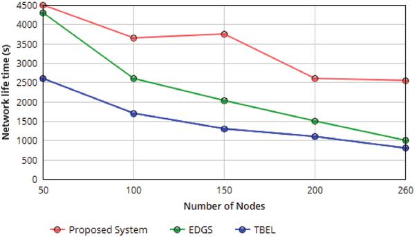
Figure 5 Life time of the network with respect varying the number of sensor nodes.

4.1 Network Lifetime

In this work, we define the network lifetime as the time the first node depleting its energy and stops working.

Figure 5 shows the network lifetime with varying number of nodes. It is observed that with the growth of the wide variety of nodes, the network lifetime decreases with Mobile Agents (MA). Because the range of MAs is fixed in terms of every curve, the growing of nodes deployed among the network node causes growing of the number of nodes on every Hop-trees. Consequently, the lifetime of the network decreases with the increasing of a wide variety of sensor nodes. The hop count value and transmission path will be less when the number of MAs used while increasing the number of sensor nodes.

4.2 Average Energy Consumption of Nodes

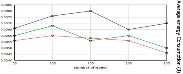
Figure 6 Average energy consumption of nodes with respect varying the number of sensor nodes.

Figure 6 shows, the average energy consumption of nodes with varying number of nodes. We address that the average energy intake of nodes while the range of MAs is 1, because a static sink positioned inside the network for node data collecting, i.e. centralized manner, therefore its energy intake is very low in this situation. The average energy intake of nodes turns into lesser with the growth of MAs.

4.3 Packet Delivery Ratio

Packet delivery ratio is defined as the ratio of number of packets successfully delivered to the destination node over the number of data packets sent by source nodes.

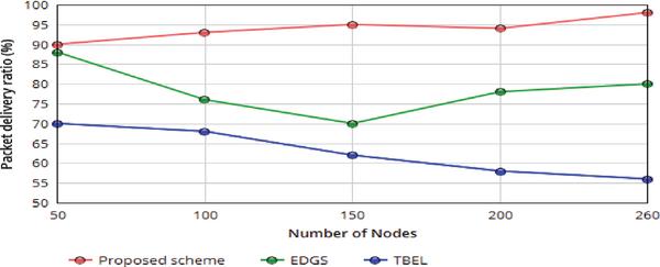
Figure 7 Packet delivery ratio of nodes with respect varying the number of sensor nodes.

Packet delivery ratio of each algorithm under varying number of nodes. We address that our proposed scheme has a higher packet delivery ratio than EDGS and TBEL. Since in the proposed scheme, when the network nodes performs efficiently, the hop count measurement and path planing to avoid the overhead and also the network nodes always updating the packet information proactively. Therefore, the packet delivery ratio is notably better than EDGS and TBEL. Initially we use lesser number of MAs used, so which results in a critical lack of packets in a few big clusters.

4.4 Simulation Results with Varying Speed of Mobile Sink

This section evaluates the impact of sink’s moving speed on network performance, the speed of mobile sink is set to 5m/s,10m/s,15m/s and 20m/s.

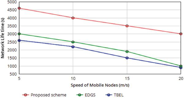
Figure 8 Network Life time with respect varying the Speed of mobile nodes.

Figure 8 shows, The average energy consumption of nodes decreases while sink movement speed increases. Since varying the speed of the mobile nodes contracts the cycle time that MAs visits sensor node or cluster head. As an end result, the ratio of proactive long-distance transmission and the strength consumption of nodes decreases. We address that average power consumption of the nodes in our proposed scheme is lower than EDGS and TBEL.

4.5 Average Computational Time Complexity

Although the proposed algorithm has optimum pattern recognition and relocalization scheme with the lowest computational time complexity.

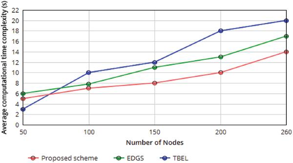
Figure 9 Average Computational time complexity with respect varying the Number of sensor node.

Figure 9 shows, The time complexity increases with a point slope, particularly for unresponsive sensor nodes. We get running time on an input of size N as a function of N, T(N) = 2T(N/2) + N. Even though the time complexity of the relocalization algorithm increases progressively with a limited range of MAs, it is not always significantly impacted by a growth inside the number of sensor nodes and their Hop counts.

5 Conclusion

In this paper, we propose an improved TBR methodology for triggering relocalization and global relocalization and data gathering algorithm through a mobile sink, it combines back-off based hop count measurement, passive uploading with local island and relocalization and data gathering with proactive uploading with global environment. We compared our proposed algorithm with other approaches in Network lifetime, Energy consumption, Packet delivery ratio and Time Complexity. The simulation results proved the effectiveness of the proposed algorithm over similar methods EDGS and TBEL. In the future work, we plan to implement security schemes for the proposed module.

References

[1] Poon, C. C., Lo, B. P., Yuce, M. R., Alomainy, A., and Hao, Y. (2015). Body sensor networks: In the era of big data and beyond. IEEE Reviews in Biomedical Engineering, 8, 4–16.

[2] Ghosh, S., and Lee, T. S. (2010). Intelligent Transportation Systems: Smart and Green Infrastructure Design. CRC press.

[3] Liu, T., and Cerpa, A. E. (2014). Data-driven link quality prediction using link features. ACM Trans. Sen. Netw. (TOSN),10(2), 37.

[4] Alam, N., and Dempster, A. G. (2013). Cooperative positioning for vehicular networks: Facts and future. IEEE Transactions on Intelligent Transportation Systems, 14(4), 1708–1717.

[5] Zhou, J., Chen, C. P., Chen, L., and Zhao, W. (2013). A user-customizable urban traffic information collection method based on wireless sensor networks. IEEE Transactions on Intelligent Transportation Systems, 14(3), 1119–1128.

[6] Yang, X., Zhang, W., and Song, Q. (2015). An improved DV-Hop algorithm based on shuffled frog leaping algorithm. Int. J. Online Engg. (iJOE)., 11(9), 17–21.

[7] Hu, Y., and Li, X. (2013). An improvement of DV-Hop localization algorithm for wireless sensor networks. Telecommun. Sys., 53(1), 13–18.

[8] Goldberg, D. (1989). Genetic algorithms in optimization, search and machine learning. Reading: Addison-Wesley.

[9] Sivasakthiselvan, S. and Nagarajan, V., (2017). Mobility Management and Adaptive Dynamic Clustering for Mobile Wireless Sensor Networks. IEEE Conference ICCSP 2017, 2246–2251.

[10] Zheng, Z., Cai, L. X., Zhang, R., and Shen, X. S. (2012). RNP-SA: Joint relay placement and sub-carrier allocation in wireless communication networks with sustainable energy. IEEE Transactions on Wireless Communications, 11(10), 3818–3828.

[11] Zhang, W., Yang, X., and Song, Q. (2015). Improvement of DV-Hop localization based on evolutionary programming resample. Journal of Software Engineering, 9(3), 631–640.

[12] Gungor, V. C., and Korkmaz, M. K. (2012). Wireless link-quality estimation in smart grid environments. Int. J. of Distributed Sensor Netw. 8(2), 214068.

[13] Prasad, R. V., Devasenapathy, S., Rao, V. S., and Vazifehdan, J. (2014). Reincarnation in the ambiance: Devices and networks with energy harvesting. IEEE Communications Surveys & Tutorials, 16(1), 195–213.

[14] Ding, Z., and Poor, H. V. (2013). Cooperative energy harvesting networks with spatially random users. In IEEE Signal Processing Lett., 20(12), 1211–1214.

[15] Cammarano, A., Petrioli, C., and Spenza, D. (2012). Pro-Energy: A novel energy prediction model for solar and wind energy-harvesting wireless sensor networks. In Mobile Adhoc and Sensor Systems (MASS), In IEEE 9th International Conference, 75–83. IEEE.

[16] Sivasakthiselvan, S., and Nagarajan, V., (2016). Design and Analysis of Estimation Algorithm for Improving Localization Performance in Wireless Sensor Networks. International Journal of Advanced Research in Computing and Information Technology, 3(2), 1–6.

[17] Pandharipande, A., and Li, S. (2013). Light-harvesting wireless sensors for indoor lighting control. IEEE Sensors Journal 13(12), 4599–4606.

[18] Niyato, D., Hossain, E., Rashid, M. M., and Bhargava, V. K. (2007). Wireless sensor networks with energy harvesting technologies: A game-theoretic approach to optimal energy management. IEEE Wireless Commun., 14(4), 90–96.

[19] Akkaya, K., Younis, M., and Bangad, M. (2005). Sink repositioning for enhanced performance in wireless sensor networks. Comp. Net., 49(4), 512–534.

[20] Zhang, P., Xiao, G., and Tan, H. P. (2013). Clustering algorithms for maximizing the lifetime of wireless sensor networks with energy-harvesting sensors. Comp. Net., 57(14), 2689–2704.

Biographies

S. Sivasakthiselvan is a Research Scholar at the Department of Electronics and Communication Engineering in Adhiparasakthi Engineering College, India. He received his B.E., and M.E. in Electronics and Communication Engineering from Anna University, India. His research interests include wireless sensor networks, with Localization and Routing.

V. Nagarajan is a Professor and Head, Department of Electronics and Communication Engineering in Adhiparasakthi Engineering College, India. He received his B.E., from Madras University, India. He received his M.Tech. and Ph.D. from Pondicherry Engineering College, India. He is a member in IEEE, ISTE, IETE, IASTE and IAE. He has published more than 150 papers in national and international conferences/journals. His research interests include wireless communication, mobile communication and signal processing.

Journal of ICT, Vol. 5_2, 129–148.
doi: 10.13052/jicts2245-800X.521
This is an Open Access publication. © 2018 the Author(s). All rights reserved.

Abstract

Keywords

1 Introduction

2 Related Works

2.1 Time Bound Essential Localization (TBEL)

2.2 Time Bound Localization (TBL)

2.3 Efficient Data Gathering System (EDGS)

3 Proposed System

3.1 System Overview

3.2 Sequence Diagram

4 Simulation Environment

4.1 Network Lifetime

4.2 Average Energy Consumption of Nodes

4.3 Packet Delivery Ratio

4.4 Simulation Results with Varying Speed of Mobile Sink

4.5 Average Computational Time Complexity

5 Conclusion

References

Biographies