Tomato: Different Leaf Disease Detection Using Transfer Learning Based Network

Siva Prasad Patnayakuni

Senior Data Engineer, H-E-B, USA
E-mail: Sivaprasadmca2021@gmail.com

Received 27 August 2021; Accepted 01 November 2021; Publication 21 January 2022

Abstract

Plant diseases have a significant effect on crop productivity, financial costs, and output. It is vital to research plant diseases in order to increase agricultural yield. Tomatoes are the world’s most frequently cultivated crop, and they are a staple ingredient in almost every cuisine. After potatoes and sweet potatoes, tomato is the most extensively cultivated vegetable on the planet. India was ranked second in tomato output. Numerous diseases have a detrimental effect on the quantity and quality of the tomato crop. Early disease detection will assist farmers in increasing crop production. The research proposes a transfer learning-based technique for detecting five distinct leaf diseases. AlexNet has been used to detect and classify disease. The simulation results reveal that the method based on transfer learning outperforms the other methods with a classification accuracy of 95.6%.

Keywords: Transfer learning, disease detection, classification, accuracy, AlexNet.

1 Introduction

Plant diseases are the primary cause of quality and quantity loss in plants/crops [1, 2]. Bacteria, fungi, and viruses are responsible for the majority of plant disease. Each year, plant diseases cause 10%–16% losses in agricultural yields worldwide, costing the global economy $220 billion. Our global population will reach 9.1 billion people in 2050, according to the FAO [3]. To feed an expanding population, agricultural output must be increased by 70%. Chemicals used to control plant diseases, such as bacteriacide and fungalcide, have a negative effect on the agroecosystem. Effective early disease detection strategies are necessary for food security and agroecosystem sustainability.

Tomatoes have grown in almost any well-drained soil [4]. Gardeners cultivate tomatoes to utilize fresh tomatoes in their homes and enjoy excellent meals. The plant development is occasionally stunted by farmers and gardeners [5]. Tomatoes may not emerge on the plant or may develop diseased black patches on the bottom. To identify tomato plant disease, first identify the infected part of the plant, secondly identify the color differences and holes on the leaf, and finally look for insects. Tomatoes and related crops like potatoes, brinjal grown three times once every year [6]. To keep soil fertile, we should grow wheat, maize, rice, sugarcane, etc., before tomato planting. Bacteria, fungus, or improper agricultural practices cause 16 illnesses, whereas insects cause 5 infections. Bacterial wilt is caused by Ralstonia solanacearum. These bacteria may penetrate roots via natural wounds produced in secondary root emergence, man-made wounds generated during cultivation. Humidity and heat promote illness growth. A bacterial slime fills the plant’s water conducting tissue by quickly proliferating. The plant’s vascular system is affected, although the leaves may remain green [7]. Infected plant stems look brown in cross section with yellowish stuff pouring out.

We present a new technique to detect illness in tomato crops by evaluating leaf images. Plant village’s tomato leaf dataset [8] has been utilized for this experiment. The study will help farmers to identify plant diseases without involving plant experts. It will help them treat plant diseases faster, improve the food crops produced, and therefore help farmers make more money.

2 Related Works

With the introduction of Deep Neural Networks (DNN), it is now possible to get promising results in plant pathology. Deep Learning (DL) based networks have been shown to substantially increase the accuracy of image categorization. In [9], proposed a machine learning model for the identification of plant disease. The accuracy of the model was significantly decreased when the testing image conditions were different from the training image circumstances. Disease may develop on the top sides of the leaves at times, and on the bottom sides of the leaves at other times. As hyper-parameters trained both AlexNet and VGG16 net using the smallest batch size, weight, and bias learning rate. In the case of VGG16net, accuracy is inversely proportional to the size of the minimum batch [10, 11].

Recently, the GMDH logistic algorithm (Group Method of Data Handling) has been developed to identify the leaf illness using data from many sources [12]. The attribute extraction procedure needed segregation in machine learning. It is a time-consuming and difficult process that has a direct impact on the performance of the classifier [13]. In large-scale data processing, DNN designs with multiple processing layers and neurons could effectively handle high-complexity tasks such as speech and picture recognition while maintaining high efficiency [14]. The use of DL techniques in the detection and segmentation of illnesses based on medicinal imageries are becoming more popular [15].

In [16], segregation of 13 distinct leaf illness using Convolutional Neural Network (CNN) has been performed. This method has been trained with 30,880 imageries and has been tested with 2589 images. The suggested model had an average accuracy of 96.3%. In [17], developed a DL based model to identify rice plant disease. Other researchers used the VGGNet module to conduct disease classification on maize and rice plants in an effort to better understand these plants’ diseases [18, 19]. Then, CNN models like as AlexNet and GoogLe Net were used to identify plant illnesses [20]. These methodologies can able to achieve a classification accuracy of 99.35%. On the other hand, when comparing the performance of Dense Net architecture with other architectures, it required less computation time. It also had the higher accuracy of 99.75% for disease classification [21].

In [22], various epochs, batch sizes, and dropouts have been used to improve the performance of their 9-layer CNN architecture. They then tested their results against the performance of common transfer learning methods. With respect to the test dataset, their suggested model obtained 96.46 percent classification accuracy. The VGG architecture utilized in the detection of plant disease and had the greatest accuracy of 99.53% [23]. Two stages of Plant Disease Net model has been developed for the classification of plant disease. In the first stage identifies the plant species from leaves, the second stage categorize the leaves. This model has given an accuracy of 93.67% [24].

In [25], novel plant detection method based on segmentation and classification was developed. LAB-based hybrid segmentation method has been used for segmentation and CNN classifier was used for classification. A novel model dubbed MobileNet-Beta has been developed by combining the previously trained MobileNetV2 model with the Classification Activation Maps had been used for plant disease detection [26]. This method given had 99.85% accuracy in the Plant Village dataset and 99.11 percent accuracy on their own dataset, according to the results of the tests. Now-a-days, DL based methodologies have been widely utilized for the plant detection of plant disease. Even though, these technique yields better results, still certain gaps that needs to be filled in terms of deep learning architectures [27]. Convolutional Neural Networks were used by pitchai et al. [32] to detect potato plant diseases. Velliangiri S et al. [33] shown that MLPA may be utilized to develop a high-accuracy and high-performance smart mushroom farm monitoring system.

Figure 1 Few sample images of the dataset.

3 Dataset

The Plant Village collection provided the dataset. Around 50,000 images of 14 different plants are included in the collection, including tomatoes, potatoes, grapes, apples, maize, blueberries, raspberries, soybeans, squash, and strawberries [28]. We chose tomato leaves with five distinct illnesses for this work. Figure 1 illustrates a few of the photos included in the dataset. Tomatoes are susceptible to a total of nine distinct illnesses. Five leaf illnesses are classified in this article, and the efficacy of the proposed strategy is examined. Around 5000 images in the training dataset, 3000 images in the validation dataset, and 500 images in the testing dataset were chosen for this experiment, with the training dataset being the largest. There are 1000 healthy photos and 1000 photographs from each of the tomato disease types described above. Each validation class comprises 700 photos, and each test class contains 50 images.

Randomly picked images from the training set are then extracted from their respective files for testing. When the number of images in a particular class is less than 1000, the data augmentation approach was used to generate some new images. The Python Augmentor package is used to generate enhanced images by rotating, flipping, cropping, and resizing existing images. When the training dataset contains more than 1000 images in a given class, we chose the top 1000 images. We used the same technique as for the training dataset to build the validation dataset, assigning 700 images to each class. This process is necessary to eliminate bias toward any particular class during CNN’s training. Each image is 256 by 256 pixels in size and is saved in the jpeg format. Table 1 contains information about the number of training and testing images.

3.1 Training and Testing Dataset

A neural network’s training and testing datasets are divided in half according to the 80:20 rule, which is the most frequently used rule in the field of neural networks [30]. The training data has been further divided into two parts: training data, which comprises 80 percent of the dataset, and validation data, which comprises 10 percent of the dataset, in order to assess the model overfitting. Each picture in the dataset is scaled to 299 $\times$ 299 pixels for both training and testing purposes in order to fit the model. Learning rate 0.001, batch size 16, momentum 0.9, and the number of epochs 15 are all hyperparameters that are utilized to train the network throughout the training process.

Table 1 Number of images

Classes	No: of Training Images	No: of Testing Images
Early blight	1666	416
Bacterial spot	1258	314
Mosaic Virus	272	68
Septoria leaf spot	1381	345
Yellow leaf curl virus	4259	1065

4 Methodology

4.1 Transfer Learning

Training a CNN Classifier requires huge number of annotated feature vectors as well as more time and computing resources than using a CNN that has already been pretrained on a big dataset. Fine tuning and freezing are the two most common transfer learning strategies. During fine-tuning, initial weights of a pretrained CNN are used in place of random initialization, and then a normal training procedure on the target dataset is conducted. In the freezing, the pretrained CNN layers extract the features from the leaf images. Then, freeze the weights and biases of convolutional layers, after that fully connected layers are fine-tuned across the target dataset. The frozen layers are not restricted to the convolutional layers in order to be effective. A subset of convolutional layers may be selected as the frozen layers in order to reduce the amount of data lost. Because of the significant disparity among the target image and the dataset, the transfer learning method has been fine tuned in order to maximize results. In this paper, pretrained AlexNet has been utilized and it has been fine tuned using plant village dataset. This AlexNet is capable leaf disease segregation, and it is significantly shallower than other CNN methods, result in faster convergence and a reduction in the amount of computational resources required for classification.

4.2 Uncertainty Score Calculation

To evaluate the efficacy from training dataset, we utilize the entropy and relative entropy metrics. The entropy formula of a discrete random variable $X$ with potential results $s_{1}, s_{2}, \dots, s_{n}$ , with probability $P (s_{1}), P (s_{2}), \dots, P (s_{n})$ , is given by the following Equation (1).

H (S) = - \sum_{i = 1}^{n} P (s_{i}) logP (s_{i})

(1)

The symmetric Kullback–Leibler (KL) divergence is the metric used for measuring the mutual information among two probability distributions on a random variables [29]. Let us consider the probability density functions $P (s)$ and $Q (s)$ over a random vector $X$ , the relative entropy may be calculated as follows using Equation (2).

D (p ∥ q) = \sum_{i = 1}^{n} P (s_{i}) \log \frac{P (s_{i})}{Q (s_{i})}

(2)

Here, the probability functions are the pretrained CNNs’ outputs.

4.3 Workflow

The block diagram of new active learning system based on transfer learning to minimize annotation costs while retaining CNN performance for leaf disease classification has been given in Figure 2. This process has the following steps:

Step 1: We chose 30% of the training data at random and assumed the other 70% are unlabeled. Then 30% labeled training subset has been pretrained using AlexNet, and varied the learning rate (i.e., 0.001, 0.0005, and 0.0001). This gave us three fine-tuned CNNs.

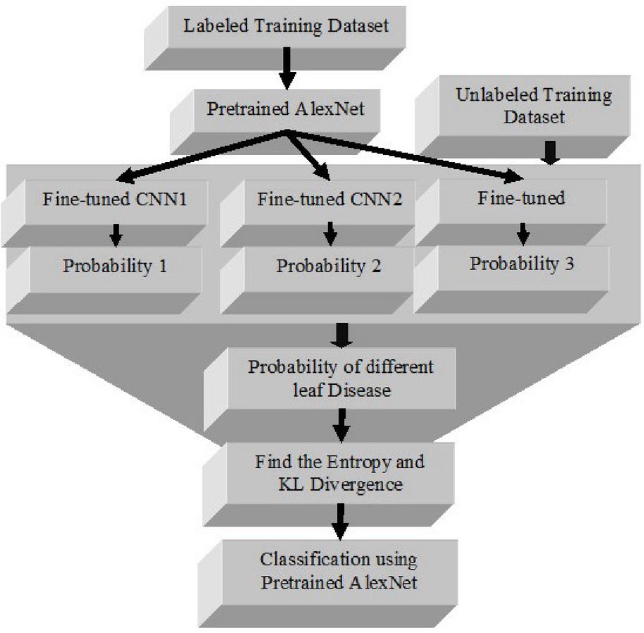
Figure 2 Workflow of transfer learning based leaf disease detection system.

Step 2: These fine-tuned CNNs calculate each sample’s categorization probability. Because the CNNs solely use forward propagation to compute outputs, no labels are needed here.

Step 3: In step 2, we calculated individual entropy and pairwise KL divergence for each training sample. Entropy and KL divergence of each sample make up the uncertainty score. This method yield an uncertainty score list for the whole training dataset.

Step 4: We selected 30% of the training cohort, which comprised of the most informative data, and sorted the uncertainty score list. This subset needed labelling and utilized to fine-tune an AlexNet. If the initial labelled training subset (30%) and the found most informative subset (30%) did not overlap, the maximum training size required is 30 $+$ 30 60% (40%) of the total training cohort. If the found most informative samples are precisely the same (30%) as the initial labelled training subset, then the maximum training size required is just 30% (70%) of the total training cohort

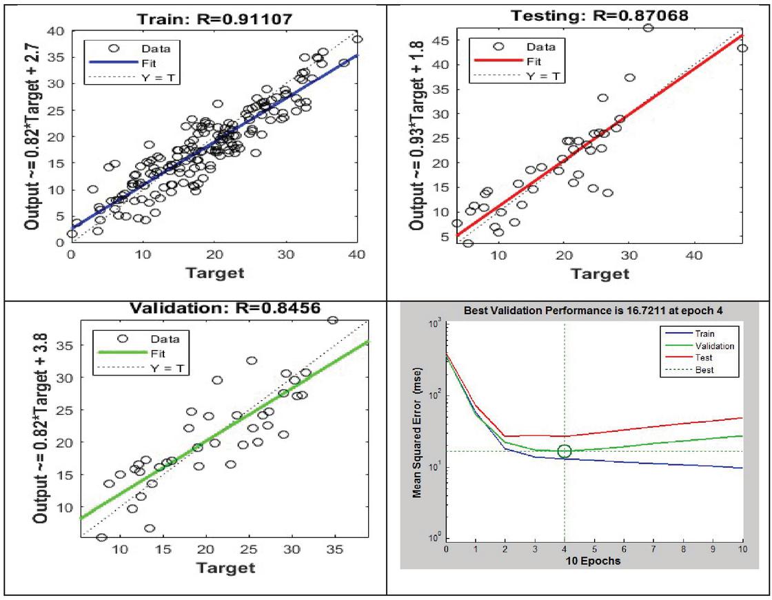
Figure 3 Training, validation, and testing phases.

5 Results and Discussion

In Figure 3, the three plots depict the data from the training, validation, and testing phases. Outputs = targets, thus the dashed line indicates the ideal outcome. An ideal linear regression line among outputs and goals is solid. The $R$ value indicates the output-to-target connection. If $R = 1$ , the outputs and targets are linearly related. The outputs and goals are not linearly related if $R$ is close to 0.

In this case, the training data shows that the model is reasonably accurate. The findings of the validation and test procedures likewise indicate high $R$ values. The scatter plot is useful in demonstrating that some data points do not fit together well. There is a data point in the test set with a network output that is near to 35, whereas the equivalent goal value is around 12. This is an example of a network output that is close to 35. Following that, it would be necessary to examine this data point in order to establish whether it reflects extrapolation of the data (i.e., is it outside of the training data set). The data should be included in the training set if this is the case, and extra data should be gathered to be utilized in the test set. Accuracy is one of the important parameter which is calculated as a percentage of the total number of predictions [30, 31]. It has been computed using the following Equation (3).

Accuracy = \frac{Number of correct predictions}{Total number of predictions}

(3)

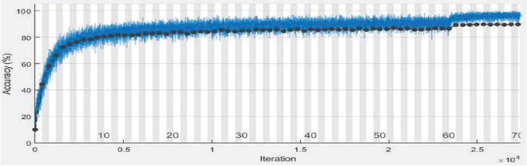
Figure 4 Accuracy of proposed method.

Figure 4 shows the best performance of the proposed methodology interms of Accuracy. From this figure, we can conclude that, the proposed method yields better performance interms of Accuracy.

6 Conclusion

Over the last several years, the agricultural sector has faced many difficulties. In this paper, it is suggested to use a transfer learning-based neural network to detect tomato leaf diseases. Specifically, this model has been created in such a manner that it may be used to identify five distinct tomato plant diseases: early blight, mosaic virus, bacterial spot, yellow leaf curl virus, and septoria spot. The experimental results showed that fine-tuning transfer learning results in a higher recognition rate than general transfer learning. This transfer learning method obtains a 95.6% of classification accuracy. In the future, the suggested model will be used to determine the severity of the tomato leaf disease, which is currently unknown. The information gained from the tomato disease classification model is also used to the detection of various plant diseases.

References

[1] Kayaa, A., Kecelia, A.S., Catalb, C., Yalica, H.Y., Temucina, H., Tekinerdoganb, B., ‘Analysis of transfer learning for deep neural network based plant classifcation models’ Comput Electron Agric, pp. 20–29, 2019.

[2] Zhang, K., Wu, Q., Liu, A., Meng, X., ‘Can deep learning identify tomato leaf disease’, Adv Multimed. pp. 1–10, 2018.

[3] Rangarajan, A.K., Purushothaman, R., Ramesh, A., ‘Tomato crop disease classifcation using pre-trained deep learning algorithm, In: International Conference on Robotics and Smart Manufacturing (RoSMa2018)’, Procedia Computer Science, pp. 1040–1047, 2018.

[4] Brahimi, M., Boukhalfa, K., Moussaoui, A., ‘Deep learning for tomato diseases: classifcation and symptoms visualization’,. Appl Artif Intell, pp. 299–315, 2017.

[5] Li, Y., Xie, X., Shen, L., Liu, S., ‘Reverse Active Learning Based Atrous DenseNet for Pathological Image Classification’ BMC Bioinformatics, pp. 1–15, 2019.

[6] Hao, R., Namdar, K., Liu, L., Khalvati, F., ‘A Transfer Learning Based Active Learning Framework for Brain Tumor Classification’. arXiv [Preprint]. Available at: https://arxiv.org/abs/2011.0926, 2020.

[7] Gowthami, K., Pratyusha, M., Somasekhar, B. ‘Detection of diseases in different plants using digital image processing’, International Journal of Scientific Research in Engineering, pp. 18–23, 2017.

[8] Hariharan, G.T., Hariharan, G.P.S., Vijay Anandh, R. ‘Crop disease identification using image processing’, International Journal of Latest Trends in Engineering and Technology, pp. 255–259, 2016.

[9] Anjna, Meenakshi Sood, Pradeep Kumar Singh, ‘Hybrid System for Detection and Classification of Plant Disease Using Qualitative Texture Features Analysis’, Procedia Computer Science, pp. 1056–1065, 2020.

[10] Kamlesh Golhani, Siva K. Balasundram, Ganesan Vadamalai, Biswajeet Pradhan, ‘A review of neural networks in plant disease detection using hyperspectral data’, Information Processing in Agriculture, pp. 354–371, 2018.

[11] Gómez-Chova, L., Tuia, D., Moser, G., Camps-Valls, G. ‘Multimodal classification of remote sensing images: a review and future directions’. Proc IEEE 2015, pp. 1560–84, 2015.

[12] Wang, G., Sun, Y., Wang, J., ‘Automatic image-based plant disease severity estimation using deep learning’, Comput Intell Neurosci, pp. 1–8, 2017.

[13] Haut, J.M., Paoletti, M., Plaza, J., Plaza, A. ‘Cloud implementation of the K-means algorithm for hyperspectral image analysis’, J Supercomput, pp. 514–29, 2017.

[14] Quirita, V.A.A., da Costa, G.A.O.P., Happ, P.N., Feitosa, R.Q., d.S. Ferreira, R.Q., Oliveira, D.A.B., ‘A new cloud computing architecture for the classification of remote sensing data’, IEEE J Sel Topics Appl Earth Observ Remote Sens, pp. 409–16, 2017.

[15] Brahimi, M., Arsenovic, M., Laraba, S., Sladojevic, S., Boukhalfa, K., Moussaoui, A., 2018. Deep learning for plant diseases: Detection and saliency map visualisation, in: Human and Machine Learning. Springer, pp. 93–117, 2018.

[16] Brahimi, M., Boukhalfa, K., Moussaoui, A., ‘Deep learning for tomato diseases: classification and symptoms visualization’, Applied Artificial Intelligence, pp. 299–315, 2017.

[17] Kalaiyarasi, M., Perumal, B., Pallikonda Rajasekaran, M. ‘Estimation of Deforestation Rate for LBA-ECO LC-14 Modeled Deforestation Scenarios, Amazon Basin: 2002–2050 using Fuzzy k-means clustering’, International Journal of Recent Technology and Engineering, pp. 2277–3878, 2019.

[18] DeChant, C., Wiesner-Hanks, T., Chen, S., Stewart, E.L., Yosinski, J., Gore, M.A., Nelson, R.J., Lipson, H, ‘Automated identification of northern leaf blight-infected maize plants from field imagery using deep learning’. Phytopathology, pp. 1426–1432, 2017.

[19] Huang, G., Liu, Z., Van Der Maaten, L., Weinberger, K.Q. Densely connected convolutional networks, in: Proceedings of the IEEE conference on computer vision and pattern recognition, pp. 4700–4708, 2017.

[20] Fujita, E., Kawasaki, Y., Uga, H., Kagiwada, S., Iyatomi, H, ‘Basic investigation on a robust and practical plant diagnostic system’, in: 2016 15th IEEE International Conference on Machine Learning and Applications (ICMLA), IEEE. pp. 989–992, 2016.

[21] Szegedy, C., Vanhoucke, V., Ioffe, S., Shlens, J., Wojna, Z, ‘Rethinking the inception architecture for computer vision’, in: Proceedings of the IEEE conference on computer vision and pattern recognition, pp. 2818–2826, 2016.

[22] Mohit Agarwal, Abhishek Singh, Siddhartha Arjaria, Amit Sinha, Suneet Gupta, ‘ToLeD: Tomato Leaf Disease Detection using Convolution Neural Network’, Procedia Computer Science, pp. 293–301, 2020.

[23] Ümit Atila, Murat Uçar, Kemal Akyol, Emine Uçar, ‘Plant leaf disease classifcation using EffcientNet deep learning model’, Ecological Informatics, p. 101182, 2021.

[24] Too, E.C., Yujian, L., Njuki, S., Yingchun, L, ‘A comparative study of fne-tuning deep learning models for plant disease identifcation’. Comput. Electron. Agric. pp. 272–279, 2019.

[25] Saleem, M.H., Potgieter, J., Mahmood Arif, K.M., 2019. ‘Plant disease detection and classifcation by deep learning. Plants’, p. 468, 2019.

[26] Perumal, B., Kalaiyarasi, M., Deny, J., Muneeswaran, V. ‘Forestry Land Cover Segmentation of SAR Image Using Unsupervised ILKFCM’, Materials today: Proceedings, 2021.

[27] Qiao, K., Liu, Q., Huang, Y., Xia, Y., Zhang, S. ‘Management of bacterial spot of tomato caused by copper-resistant Xanthomonas perforans using a small molecule compound carvacrol’. Crop. Prot. p. 105114, 2020.

[28] Abdulridha, J., Ampatzidis, Y., Kakarla, S.C., Roberts, P. ‘Detection of target spot and bacterial spot diseases in tomato using UAV-based and benchtop-based hyperspectral imaging techniques’. Precis. Agric. pp. 955–978, 2020.

[29] Calleja-Cabrera, J., Boter, M., Oñate-Sánchez, L., Pernas, M. ‘Root growth adaptation to climate change in crops’. Front. Plant. Sci. p. 544, 2020.

[30] Choi, H., Jo, Y., Cho, W.K., Yu, J., Tran, P.-T., Salaipeth, L., Hae-Ryun, K., Hong-Soo, C., Kook-Hyung, K. ‘Identification of Viruses and Viroids Infecting Tomato and Pepper Plants in Vietnam by Metatranscriptomics’. Int. J. Mol. Sci. p. 7565, 2020.

[31] Kalaiyarasi, M., Perumal, B., Pallikonda Rajasekaran, M., Saravanan, S. ‘Color-Based SAR Image Segmentation Using HSV $+$ FKM clustering for Estimating the Deforestation Rate of LBA-ECO LC-14 Modeled Deforestation Scenarios, Amazon Basin: 2002–2050’, Arabian Journal of Geosciences, p. 777, 2021.

[32] R, P., Kumar G, S., Varma D, A., CH, M. B. ‘Potato Plant Disease Detection Using Convolution Neural Network’. International Journal of Current Research and Review, 12(20), 152–156, 2020.

[33] Velliangiri, S., Sekar, R., Anbhazhagan, P. ‘Using MLPA for smart mushroom farm monitoring system based on IoT’, International Journal of Networking and Virtual Organisations, 22(4), 334–346.

Biography

Siva Prasad Patnayakuni is currently working as Senior Data Engineer in HEB. His current research focus is on Distributed Data, Cloud Computing & Predictive Analytics and recommendations. He holds his Bachelor’s degree in Computer Sciences from Andhra University, India in 1996 and Masters in Computer Applications from Osmania University in 1999. He has been successfully designing and building large scale data warehousing, data pipelines, real-time analytics, reporting solutions for complex business problems. He created an intuitive architecture/framework that helps organizations on effectively analyzing large scales of structured & unstructured data.