A Prototype Similarity-based System for Remaining Useful Life Estimation for Future Industry by Singular Spectrum Analysis-Long Short Term Memory Neural Networks Algorithm
Prakit Intachai1,* and Peerapol Yuvapoositanon2
1The Electrical Engineering Graduate Program, Faculty of Engineering, Mahanakorn University of Technology,140 Cheumsamphan Rd., Nong-chok Bangkok 10530, Thailand
2Mahanakorn Institute of Innovation, Faculty of Engineering, Mahanakorn University of Technology,140 Cheumsamphan Rd., Nong-chok Bangkok 10530, Thailand
E-mail: prakit2554@gmail.com; peerapol@mutacth.com
* Corresponding Author
Received 29 November 2019; Accepted 26 May 2020; Publication 14 August 2020
Abstract
In this paper, we propose a prototype similarity-based approach of estimating the remaining useful life (RUL) of turbofan engine data using the singular spectrum analysis and the long-short term memory (SSA-LSTM) neural networks algorithm. The algorithm consists of two steps. First, the optimal window length of the trajectory matrix of the dataset is empirically determined from a prototype dataset. Second, the estimation of the RUL of the target datasets is performed using the window length parameter obtained from the first step. The validity of the proposed algorithm is verified by testing with 200 turbofan engine datasets. The results are shown to have a significant improvement in the performance of the RUL estimation over the existing LSTM algorithm.
Keywords: Remaining useful life, Singular spectrum analysis, Long-short term memory, Optimal window length.
1 Introduction
Recently, predictive approaches for estimating remaining useful life (RUL) of a device or a machine have gained increasing interest in the maintenance perspectives [1,2]. The reliability of these approaches depends on the accuracy of the RUL estimation. However, the RUL estimation is generally difficult in practice because some devices may not be suitable for physics-based estimation of true RUL when the real-life system is complex [3], or the characteristic of some time series data is described as non-linear [4]. Different techniques can be used in order to estimate the RUL, such as the data-driven methodology in Ref. [5], and similarity methods presented in Refs. [6–8]. The data-driven models are more suitable in some cases where supported models for the RUL are not achievable.
The singular spectrum analysis (SSA) is a decomposition technique for general time series [9]. The SSA decomposition process is data-adaptive and does not involve any harmonic function. Therefore, the SSA is suitable to perform on non-linear and non-stationary time series. The noise of time series in the process of the SSA can be described as definition of window length (L) [10] when L is an integer for creating the trajectory matrix. In Ref. [11], shown the estimation of L∼T/2 is shown when T is the total number of data in the time series. The estimated window length (Lest) or L∼T/2 is a simple method of choosing L. Elsner and Tsonis [12] present some dialogue and remark that choosing Lest = T/4 is a common method, and L from that method is not larger than Lest = T/2. A method of L selection states that a suitable parameter for L should depend on Lest < T/2 as presented in Ref. [13]. In Ref. [14], L selection is described as Lest = log(T)c with c ∈ (1.5, 3.0). Moment test for L selection in the SSA [15] is presented for the method of determining Lest by a statistical test, with described as the estimated window length. Therefore, in order to do that each of the datasets must be estimated separately. For a set of time series, there is no existing approach suggesting an estimated window length optimally for the group of datasets. However, the length L is large when a time series is long. Also, for a system that has to deal with many time series, it is not practical for determining L for every time series.
In this paper, we propose an algorithm for the RUL estimation of multiple target time series with the LSTM network by means of the basis functions decomposed from the prototype time series using the SSA. The LSTM is adopted in our approach since its usages in the RUL estimation have been widely studied in the literature [16, 17]. By this approach, determining L for the target time series can be performed using the information derived from the prototype time series. The window length L optimal or Lopt for the prototype time series is achieved at the point where the root mean square error (RMSE) obtained from the LSTM is minimized. For the target time series, which will be shown later, that can be reconstructed from the prototype basis function with scaling factor, the same optimal window length Lopt can also be applied. The proposed system offers the advantage of determining the optimal parameters for a large number of time series using only those determined from the representative one called the prototype. The proposed technique is therefore a multi-step approach for the RUL estimation of a target time series using the LSTM with transformed basis functions obtained from the prototype time series. Since the subcomponents of the prototype time series are obtained from the SSA, this algorithm is called the SSA-LSTM algorithm.
The organization for the remaining of the paper is as follows. In Section 2, the definition of the trajectory matrix of a dataset, the window length and the basis functions are presented. In Section 3, the relationships between the prototype and target datasets via the basis functions and their coefficients are described. The construction of the SSA-LSTM algorithm and the determination of the window length are defined. Finally, Section 4 shows how the validity of the proposed algorithm in the prototype similarity-based RUL estimation is tested for the turbofan datasets acquired from Ref. [18]. Finally, conclusions are provided in Section 5.
2 Methodology
2.1 The Diagonal Averaging Parameters and their Coefficients
The ability of the SSA is mentioned in Ref. [10]. The SSA can be applied to the stationary and non-stationary time series data because it can describe what time series with no a priori information about the data structure. The SSA technique is based on the singular value decomposition (SVD) of the trajectory matrix of the SSA [10]. The model of the trajectory matrix can be expressed as
| (1) |
where X denotes the trajectory matrix and x(t), t = 1, 2, ⋯, T is the time series data of interest. L is the window length and 1 < L < T − 1 defines the number of rows in X. K is the embedding dimension and K = T − L + 1 where T is the time interval of the observed time series data. The trajectory matrix of X is processed by the SVD, and the matrices U, D and VT are derived in the process of decomposition as
| (2) |
where D denotes the eigenvalues matrix of svd(X), and the value of eigenvalues is expressed in the diagonal matrix as D = diag(λ1, λ2, ⋯, λL). U and V are the eigenvectors matrices. .
The eigentriple can be applied to the process of eigentriple grouping and diagonal averaging of the SSA [10, 11]. θi(t) describes the result from the process of diagonal averaging as where L is the parameter to be determined.
3 Prototype and Target Time Series
3.1 The Basis Function and its Coefficient
In this section, we explain the idea of how to represent a time series, called the target, using the basis functions derived from another time series, called the prototype.
The hypothesis underlying this idea stems from the concept of basis functions in Fourier series of a periodic time series [19]. First, the estimates of the prototype and the target time series are determined from
| (3) |

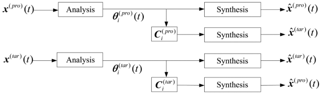
Figure 1 The concept of representing the target time series x̂(tar)(t) from the diagonal averaging parameters , and their coefficients from the prototype time series through the analysis and synthesis parts of SSA, is illustrated. The reverse operation, i.e., representing the prototype from the target, is also shown.
| (4) |
where and denote the diagonal averaging results from the basis function x̂(pro) and x̂(tar) of the prototype and the target, respectively.
Now the relationship between the prototype and the target can be described as
| (5) |
| (6) |
where
| (7) |
is the coefficient matrix required for reconstructing x̂(pro)(t) from and
| (8) |
is the coefficient matrix required for reconstructing x̂(tar)(t) from . This relationship can be depicted through the analysis and synthesis operations of the SSA in Algorithm 1.

3.2 Reconstruction of a Time Series from a Group of Subcomponents
Operating on the separated groups of the SSA data can lead to an enhanced performance [20, 21]. Therefore, we divide the analysis components into three groups as follows
| (9) |
where x̂p(t) denotes the pth group of the sub-component x̂(t) which in turn is the estimated version of x(t) and B is an integer designating the number of components in the second group, p = 2. The choice of B can be changed as B = 3, 4, 5 or B = 3, 4, ⋯, L − 1. From (9), the estimate of x(t) can be achieved by the summation of the three groups:
| (10) |
3.3 Estimation Model for Reconstructed Data
The combination of the SSA and neural networks has been studied in the literature [22, 23] and the results of estimation performance are improved as compared to those from using only the neural networks. It was shown that the LSTM is promising for the estimation of trendy time series [16, 17]. Since the RUL datasets of multiple turbo fan engines time series [18] is trendy, the LSTM is then adopted as the neural network algorithm of the estimation part in our proposed SSA-LSTM architecture for the RUL estimation.
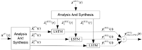
In Figure 2, the schema of the SSA-LSTM architecture is illustrated. The datasets, which are arranged as time series, are categorized as features of x(F) (t) and their associated RULs x(RUL) (t) have gone through the analysis and synthesis of the SSA resulting in groups of the reconstructed datasets , and for p = 1, 2, 3 for feature and RUL datasets, respectively. x̂(RUL)(t) is the training datasets to the LSTM networks whose outputs , p = 1, 2, 3 are the estimation results of the three LSTM networks. The estimate of the true RUL is simply the combination of :
| (11) |
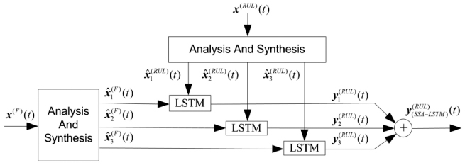
Figure 2 The proposed SSA-LSTM algorithm for RUL estimation is illustrated. Three sub-components of features, and from analysis and synthesis parts of SSA are used by the LSTM in order to generate the estimated RUL .
The process of determining the optimal value of L, the Lopt, involves analysis and synthesis of both the features and true RUL of the prototype turbofan engine datasets [18]. The three LSTM networks are fed with the synthesized sub-components of the features x̂(F)(t) and are trained with the synthesized sub-components of the true RUL. The root mean squared errors (RMSE) of the prediction for all possible values of L up to T/2, i.e., Lest = T/2, are measured. The values of L at the minimum RMSE is then selected as the optimal data-dependent L, i.e., Lopt.

We also show that considering the similarity between the prototype and the targets, Lopt that is obtained from the prototype can be applied to the analysis and synthesis parts of the SSA of the targets as well.
4 Experimental Results
4.1 The Data Sets
The data sets for the experiments were the turbofan engine degradation simulation dataset provided by the Prognostics CoE at the NASA Ames Research Center [18]. In the datasets obtained from Ref. [18], there are 200 datasets recorded from several sensors under different conditions of both normal and fault modes. Features and RULs datasets are also provided. In order to cope with different scales experienced in the datasets, we apply the normalization process before performing the RUL estimation. Ref. [24] describes how the turbofan engines are used. Let x″(F)(t) and be a raw dataset and its time average respectively and σ be the standard deviation of x″(F)(t) from various sensor measurements, then its feature and normalized version can be calculated by
| (12) |
| (13) |

where x′(F)(t) and x(F)(t) are the features and its normalized version of the raw data x″(F)(t), respectively. The maximum and the minimum of x′(F)(t) are defined by and , respectively. The normalized feature x′(F)(t) is fed to the analysis and synthesis operations by the SSA to produce the basis functions act as in Figure 2.
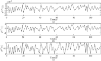
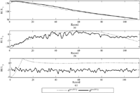
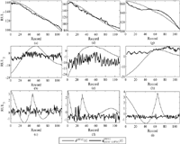
In Figures 3(a)–(c), an example of x″(F)(t) is compared with its feature and normalized version, x′(F)(t). In this section, we explain the idea of how to represent a time series, called the target.
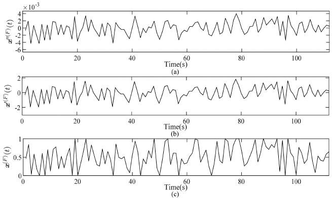
Figure 3 An example of a date set to be used as a feature which is categorized into (a) raw dataset, (b) the feature and (c) the normalized feature.
4.2 Optimal Window Length of Prototype Data and Performance Metrics
In this section, we provide an empirical approach in determining the optimal window length Lopt and the value of B of the prototype data. The performance metrics are the mean absolute error (MAE) and the RMSE defined respectively as
| (14) |
| (15) |
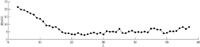
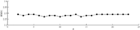
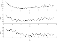
where x(RUL)(t) is the true RUL data and is the RUL estimate of the SSA-LSTM algorithm as shown in Figure 2. In our similarity-based approach, Lopt is calculated from a dataset, namely the prototype data, selected from the 200 datasets. The true RUL datasets contain T= 116 records. From Ref. [11], the estimate maximum range of the window length to be used for the trajectory matrix X in (1), Lest, is determined by Lest = T/2, i.e., Lest= 58. The RMSE of the estimated RUL of the prototype data for 3 ≤ L ≤ 57 is plotted in Figure 4. It is noted that for this particular prototype data, Lopt is 24 since the minimal RMSE is attained at that point. This value of Lopt coincides with the suggested values of Lopt < T/2 of Ref. [13], Lopt = T/4 of Ref. [12], Lopt = log(T)c of Ref. [14] and of Ref. [15]. In finding the value of B, we fixed Lopt = 24 and varied B from 3 to 23. However, as shown in Figure 5, the sensitivity of the RMSE of the estimation RUL to B is low. This means that we can choose from a wide degree of freedom.
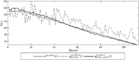
In Figures 6 and 7, the estimation of the basis functions of the and the estimation of true RUL x(pro, RUL)(t) of the prototype are shown respectively using Lopt = 24 and B = 9.
In Figure 6, the thin lines are the true RUL basis functions and the thick lines are the estimated true RUL outputs from the LSTM networks . As shown in Figure 6(a), the estimated RUL for p= 1, i.e., is able to track the true RUL . However, for the second and third estimated basis functions, i.e., and , respectively, the tracking errors are higher than the first.
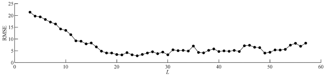
Figure 4 The RMSE of estimated RUL for prototype data for 3 ≤ L ≤ 57.
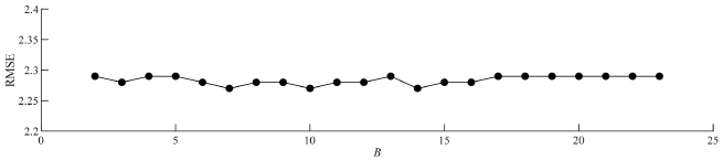
Figure 5 RMSE of the estimated RUL for various values of B.
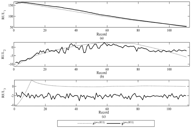
Figure 6 Estimated RULs of three sub-components for the prototype data, , are provided in (a) , (b) and (c) .
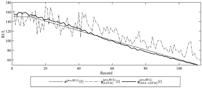
Figure 7 Estimated RUL of prototype data by SSA-LSTM using the optimal windows length Lopt = 24 and B = 9.
Nevertheless, after all the estimated RULs for the sub-components are combined to form y(pro, RUL)(t) to the estimated true RUL as described in (11), the RMSE in tracking RUL of the proposed SSA-LSTM algorithm was 2.285, whereas that of the LSTM [24] was 23.24.
4.3 Testing on the Target Datasets
In order to test the concept of the proposed similarity based RUL prediction system, we then tested whether the remaining datasets respond to the choice of window lengths in similar ways to the prototype. We selected 20 datasets from the remaining 199 datasets and measured the RUL estimation performance of each dataset at various choices of the window length, L.
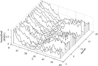
In Figure 8, the normalized RMSE plots of the selected 20 datasets are illustrated. It is interesting to observe that the window lengths associating with low RMSE of all 20 datasets are approximately in the range of 10 to 30. The regions coincide with the suggested window lengths as stated in Refs. [11–15]. As the optimal window length obtained from the prototype data, Lopt was 24, it is legitimate for using Lopt as a representative for the window length for all the target datasets selected from the remaining datasets.
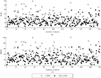
Proceeding to the evaluation of the SSA-LSTM algorithm, we tested the performance for 200 datasets as compared to the existing LSTM algorithm. We used the optimal window length Lopt = 24 for the SSA-LSTM algorithm. The additional parameter to be set for the SSA-LSTM was B which was set to nine. The performance metrics were the MAEs and the RMSEs of the RUL estimation of the SSA-LSTM and LSTM algorithms, and are shown in Figures 9(a) and 9(b), respectively. The black circles denote the results from using the SSA-LSTM, whereas those from the LSTM are represented by the white ones. As shown in Figures 9(a) and 9(b), both the MAE and RMSE levels of the SSA-LSTM are lower in average across the 200 datasets as compared to those of the LSTM. The numerical results of the averaged MAEs and RMSEs for the 200 datasets of both the algorithms are shown in Table 1. The numerical results indicate that those of the SSA-LSTM are lower than those of the LSTM nearly by half.

Figure 8 The ensemble of the normalized RMSEs in RUL estimations of 20 target datasets performed by the proposed SSA-LSTM algorithm.
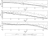
We then investigated in detail regarding how the SSA-LSTM and LSTM perform comparatively in estimation of the RUL in each record. We selected three target datasets from 199 datasets and labeled them tar1 to tar3. Similar to Figure 8, the RMSEs of three target datasets were tested against the window lengths as shown in Figures 10(a)–(c). It is shown that the window length associated with the minimum RMSEs of all tar1 to tar3 datasets are located in the vicinity of Lopt obtained from the prototype datasets, i.e., Lopt = 24.
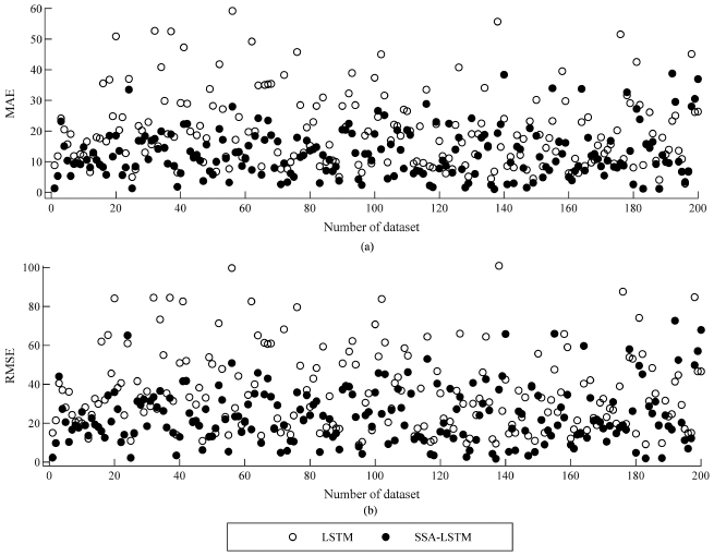
Figure 9 Performance plots of RUL estimation of 200 datasets by SSA-LSTM, (black circles) and LSTM (white circles) as measured by (a) the mean absolute errors (MAEs) and (b) the root mean squared errors (RMSEs).
Table 1 Averaged MAE and averaged RMSE for 200 datasets
| Algorithms | MAE | RMSE |
| LSTM | 23.828 | 35.284 |
| SSA-LSTM | 12.750 | 19.783 |
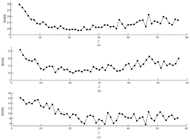
Figure 10 The RMSE at various window lengths of (a) tar1, (b) tar2 and (c) tar3
Also, the parameter B was set to nine. In Figures 11(a)–11(i), the three sub-components of the true RUL, , i.e., p= 1, 2, 3 are estimated by the SSA-LSTM. Figures 11(a)–11(c) illustrate the estimation results for the first target datasets tar1 of and where p= 1 to 3, respectively. In a similar fashion, Figures 11(d)–11(f) are the results p= 1 to 3 for the second target tar2 and Figures 11(g)–11(i) are for the third target tar3.
For all the three sub-component RUL data, the SSA-LSTM performs the best in the estimation of for the first sub-component RUL , and the same are shown in Figures 11(a), (d) and (g). This is true for all the three targets, tar1–3, even though the performance of tar3 is not as good as those of the other two. For the sub-component and , the estimation and witness the degradations in performance. However, after combining all the sub-components to produce the estimated RUL, , the SSA-LSTM shows a more promising result in the RUL estimation than the LSTM. The results are shown in Figures 12(a)–12(c).
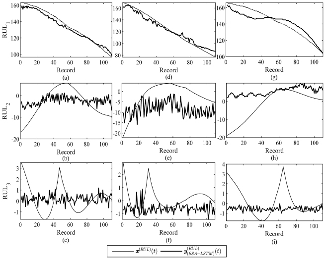
Figure 11 The estimated sub-components RULs of three target datasets by SSA-LSTM with Lopt = 24 and B = 9 for (a,b,c) tar1, (d,e,f) tar2 and (g,h,i) tar3.
By inspection, it is apparent that for all the three target datasets, the SSA-LSTM algorithm is capable of estimating the RULs, whereas the LSTM has a difficulty in performing the task. For numerical results the MAEs and RMSEs of the RUL prediction of the SSA-LSTM and LSTM are compared in Tables 2 and 3, respectively.
It is apparent from the results of the MAE and RMSE for all the three target datasets that the SSA-LSTM has achieved a significant improvement over the LSTM.
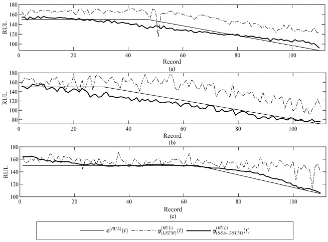
Figure 12 The estimated RUL of three target datasets by SSA-LSTM and LSTM for (a) tar1, (b) tar2 and (c) tar3.
Table 2 MAE of RUL estimation by LSTM and SSA-LSTM for the three target datasets
| Algorithm | |||
| LSTM | 24.4638 | 26.8894 | 12.7456 |
| SSA-LSTM | 6.9426 | 9.7874 | 4.7874 |
Table 3 RMSE of RUL estimation by LSTM and SSA-LSTM for the three target data sets
| Algorithm | |||
| LSTM | 26.8622 | 28.5992 | 14.2143 |
| SSA-LSTM | 8.1145 | 10.8742 | 5.8742 |
5 Conclusion
In this paper, we have proposed the SSA-LSTM for the estimation of the RUL of turbofan engines’ datasets of Ref. [18]. The proposed system offers the advantage of determining the optimal parameters for a large number of datasets using only those determined from one representative dataset called the prototype. The algorithm is a two-step approach. First, the optimal window length of the trajectory matrix of the data is empirically determined from a prototype dataset. This involves the analysis and synthesis operations of the SSA algorithm and the estimation part of the LSTM networks. Second, the target datasets are selected for the RUL estimation with the SSA-LSTM algorithm using the optimal window length obtained from the first part.
The experimental results show how the performance in RUL estimation of the proposed system has improved significantly over the existing LSTM. The validity of this concept is verified by testing on 200 datasets of features and true RULs of the turbofan engines.
References
[1] L. Ren, Y. Sun, H. Wang, and L. Zhang. Prediction of bearing remaining useful life with deep convolution neural network. IEEE Access, 6:13041–13049, 2018.
[2] Z. Zhao, B. Liang, X. Wang, and W. Lu. Remaining useful life prediction of aircraft engine based on degradation pattern learning. Reliability Engineering & System Safety, 164:74–83, 2017.
[3] Y. Liu, X. Hu, and W. Zhang. Remaining useful life prediction based on health index similarity. Reliability Engineering & System Safety, 185:502–510, 2019.
[4] X.S. Si, W. Wang, C.H. Hu, D.H. Zhou, and M.G. Pecht. Remaining useful lifeestimation based on a nonlinear diffusion degradation process. IEEE Transactions on Reliability, 61(1):50–67, 2012.
[5] E. Sutrisno, H. Oh, A. S. S. Vasan, and M. Pecht. Estimation of remaining useful life of ball bearings using data driven methodologies. In 3rd IEEE Conference on Prognostics and Health Management, Denver, Colorado, 18-21 June, 2012, pages 1–7, June 2012.
[6] F. Liu, B. He, Y. Liu, S. Lu, Y. Zhao, and J. Zhao. Phase space similarity as a signature for rolling bearing fault diagnosis and remaining useful life estimation. Shock and Vibration, 2016(5341970):1–12, 2016.
[7] Q. Zhang, P. W.T. Tse, X. Wan, and G. Xu. Remaining useful life estimation for mechanical systems based on similarity of phase space trajectory. Expert Systems with Applications, 42(5):2353–2360, 2015.
[8] L. Zeming, G. Jianmin, J. Hongquan, G. Xu, G. Zhiyong, and W. Rongxi. A similaritybased method for remaining useful life prediction based on operational reliability. Applied Intelligence, 48(9):2983–2995, 2018.
[9] P. Bonizzion and J.M.H. Karel. Singular spectrum decomposition: A new method for time series decomposition. Advances in Adaptive Data Analysis, 6(4):1450011, 2014.
[10] N. Golyandina and A. Zhigljavsky. Singular Spectrum Analysis for time series. Springer Science & Business Media, 2013.
[11] N. Golyandina and A. Korobeynikov. Basic singular spectrum analysis and forecasting with r. Computational Statistics & Data Analysis, 71:934–954, 2014.
[12] J.B. Elsner and A.A. Tsonis. Singular spectrum analysis: a new tool in time series analysis. Springer Science & Business Media, 2013.
[13] M. Atikur Rahman Khan and D.S. Poskitt. A note on window length selection in singular spectrum analysis. Australian & New Zealand Journal of Statistics, 55(2):87–108, 2013.
[14] M.A.R. Khan and D. Poskitt. Window length selection and signal-noise separation and reconstruction in singular spectrum analysis. Monash Econometrics and Business Statistics Working Papers, 23(11):2011-23, 2011.
[15] M.A.R. Khan and D. Poskitt. Moment tests for window length selection in singular spectrum analysis of short-and long-memory processes. Journal of Time Series Analysis, 34(2):141–155, 2013.
[16] W. Mao, J. He, J. Tang, and Y. Li. Predicting remaining useful life of rolling bearings based on deep feature representation and long short-term memory neural network. Advances in Mechanical Engineering, 10(12):1687814018817184, 2018.
[17] J. Liu, Q. Li, W. Chen, Y. Yan, Y. Qiu, and T. Cao. Remaining useful life prediction of pemfc based on long short-term memory recurrent neural networks. International Journal of Hydrogen Energy, 44(11): 5470–5480, 2019.
[18] NASA. Prognostics Center of Excellence Data Repository: Turbo-fan engine degradation simulation data set. https://ti.arc.nasa.gov/tech /dash/groups/pcoe/prognostic-data-repository/, last accessed on May 2020.
[19] F.J. Harris. On the use of windows for harmonic analysis with the discrete fourier transform. IEEE, 66:51–83, 1978.
[20] A. Miranian, M. Abdollahzade, and H. Hassani. Day-ahead electricity price analysis and forecasting by singular spectrum analysis. IET Generation, Transmission & Distribution, 7(4):337–346, 2013.
[21] C. Yu, Y. Li, and M. Zhang. Comparative study on three new hybrid models using elman neural network and empirical mode decomposition based technologies improved by singular spectrum analysis for hour-ahead wind speed forecasting. Energy Conversion and Management, 147:75–85, 2017.
[22] C. Lima, V.L. de Oliveira Castellani, J.F.M. Pessanha, and A. Soares. A model to forecast wind speed through singular spectrum analysis and artificial neural networks. In Proceedings on the International Conference on Artificial Intelligence (ICAI), The Steering Committee of The 2017 World Congress in Computer Science, Computer Engineering and Applied Computing, Las Vegas, Nevada, USA, 17-20 July, 2017, pages 235–240, July 2017.
[23] P. Intachai and P. Yuvapoositanon. A singular spectrum analysis pre-coded deep learning architecture for forecasting currency time series. In 6th International Electrical Engineering Congress (iEECON), Krabi, Thailand, 7-9 March, 2018, pages 1–4. IEEE, Mar 2018.
[24] The Mathworks Inc.. Sequence-to-sequence regression using deep learning. https://www.mathworks.com/help/deeplearning/ug/sequence-to-sequence-regression-using-deep-learning.html, last accessed on May 2020.
Biographies

Prakit Intachai received his bachelor’s and master’s degrees in telecommunication engineering in 2010 and 2012, respectively. Currently, he is pursuing a doctor of engineering degree in electronic engineering with signal processing as the subject of study at the Mahanakorn University of Technology, Bangkok, Thailand. His main research interests include technical analysis and synthesis of time series data and estimation of remaining useful life in industrial systems.

Peerapol Yuvapoositanon received his B.Eng degree in electronics from the King Mongkut’s Institute of Technology, Ladkrabang, Thailand in 1991 and the M.Sc., degree and DIC in physical science and engineering in medicine in 1995 and Ph.D. degree and DIC in electrical engineering (digital signal processing for wireless communications) in 2002, both from the Imperial College, London, United Kingdom. Since 1992, he has been with the Mahanakorn University of Technology, Bangkok, Thailand where he is now serving as an associate professor in electronic engineering. Throughout the years, he has served as a reviewer and a technical program committee member for multiple international conferences and journals. He has also been involved in the automation industry as a consultant for image and signal processing tasks. His current research interests include signal processing theory for time series analysis in predictive maintenance and machine learning algorithms for industrial applications.
Journal of Mobile Multimedia, Vol. 16_1-2, 181–202.
doi: 10.13052/jmm1550-4646.16129
© 2020 River Publishers