Distributed JPEG Compression and Decompression for Big Image Data Using Map-Reduce Paradigm
U. S. N. Raju*, Hillol Barman, Netalkar Rohan Kishor, Sanjay Kumar and Hariom Kumar
Department of Computer Science and Engineering, National Institute of Technology Warangal, Warangal, Telengana State, India – 506004
E-mail: usnraju@nitw.ac.in; hillol7797@gmail.com; netalkarrohan@gmail.com; sanjayamystery@gmail.com; hkmc18120@student.nitw.ac.in
*Corresponding Author
Received 24 October 2021; Accepted 20 February 2022; Publication 30 June 2022
Abstract
Digital data is primarily created and delivered in the form of images and videos in today’s world. Storing and transmitting such a large number of images necessitates a lot of computer resources, such as storage and bandwidth. So, rather than keeping the image data as is, the data could be compressed and then stored, which saves a lot of space. Image compression is the process of removing as much redundant data from an image as feasible while retaining only the non-redundant data. In this paper, the traditional JPEG compression technique is executed in the distributed environment with map-reduce paradigm on big image data. This technique is carried out in serial as well as in parallel fashion with different number of workers in order to show the time comparisons between these setups with the self-created large image dataset. In this, more than one Lakh (121,856) images are compressed and decompressed and the execution times are compared with three different setups: single system, Map-Reduce (MR) with 2 workers and MR with 4 workers. Compression on more than one Million (1,096,704) images using single system and MR with 4 workers is also done. To evaluate the efficiency of JPEG technique, two performance measures such as Compression Ratio (CR) and Peak Signal to Noise Ratio (PSNR) are used.
Keywords: Big image data, map-reduce, distributed environment, JPEG compression, JPEG decompression.
1 Introduction
The use of mobile phones and digital hand-held cameras has increased exponentially in recent years, resulting in a massive image dataset. Maintaining such a vast image library is a time-consuming and difficult task. To store such a large image dataset, an efficient approach is necessary. Image compression is one of the most effective solutions to such issues. Image compression is the process of reducing the amount of data required to represent the image and remove the redundant data. The possible redundancies in an image are Coding redundancy, Spatial and temporal redundancy and irrelevant information [1]. The whole process of compression and decompression is shown in Figure 1. The image compression can be lossy or lossless depending on the method used to remove the redundancy. Image compression is the process of shrinking image data files while maintaining essential information. The compression ratio is the ratio of the original, uncompressed image file to the compressed image file. Compression of image data can be done in spatial domain, frequency domain or in wavelet domain. Different algorithms use the data from different domains. In this paper JPEG algorithm for both compression and decompression is used with Map-Reduce paradigm by considering multiple workers.
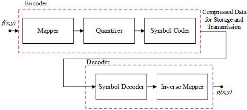
Figure 1 Block diagram of image compression system.
Image Data in Frequency Domain: The rate at which the value of pixels in the spatial domain changes is represented by the frequency domain representation of an image. The Discrete Fourier Transform (DFT) or Discrete Cosine Transform (DCT) can be used to convert an image from the spatial domain to the frequency domain. Equation (1) can be used to compute the 2-dimensional DFT of an image, and Equation (2) can be used to compute the Inverse Discrete Fourier Transform (IDFT) of an image of size MN.
| (1) | |
| (2) |
where 0=uM and 0=vN, 0=xM and 0=yN, represents an image and represents the DFT transform of the image. DFT has both real and imaginary components. With the help of DCT, the image can be represented in the frequency domain in a different way, using only the real part. DCT has a greater energy compaction than DFT, which allows it to represent the majority of energy coefficients in a sequence with only a few transform coefficients. This makes it more suitable for feature extraction. As a result, DCT is better suited for feature extraction than DFT. Equations (3) and (4) offer the equations for performing the DCT and Inverse Discrete Cosine Transform (IDCT) on an image (4).
| (3) | ||
| (4) |
where 0=uM and 0=vN, 0=xM and 0=yN, represents an image and represents the DCT transform of the image. Image enhancement, restoration, compression, watermarking, representation & description, and CBIR can all benefit from the frequency domain properties. For CBIR, Kazuhiro Kobayashi et al. [2] exploited frequency domain characteristics. For feature extraction of CBIR, Jose A. Stuchi et al. [3] used frequency domain layers of CNN architecture.
Initially the compression methods reduced the statistical redundancy by using the entropy coding of the image, arithmetic coding [4], Golomb coding [5] and Huffman coding [6]. Fourier transform [7] and Hadamard transform [8] were later proposed in late 1960s that transform the images from spatial domain to frequency domain and Discrete Cosine Transform (DCT) [9] proposed by Ahmed et al. in 1974 proves compression becomes more efficient when considering only the low frequency domain image energy. Later, quantization and prediction techniques were proposed in image compression which further reduced visual and spatial redundancies of an image. The most well-known and used algorithm is the JPEG compression standard. Apart from DCT, JPEG uses differential pulse code modulation (DPCM) [10]. JPEG 2000 [11], another image compression standard uses 2D wavelet transform to represent images instead of DCT and uses arithmetic coding EBCOT [12] to lower statistical redundancy.
Big Image Data Processing: Digital devices have progressed from having very little storage capacity, processing power, and a larger size to having greater storage, processing power, and a smaller size. As a result of this progress, these digital gadgets now generate a large amount of diverse and complex data. As a result, current computing equipment are capable of storing and analysing such information. The first fields to encounter such a data explosion were astronomy and genomics, which originated the term BigData [13]. Big is a moving target that cannot be quantified. What is considered ‘Big’ today may not be so in the future. Volume, Variety, and Velocity are three characteristics that can be found in ‘Big Data’. It is important to note that this does not imply that it must possess all three features. The number of Vs grew with time, reaching 4Vs in 2012, 7Vs in 2013 [14], and 10Vs in 2014 [15].
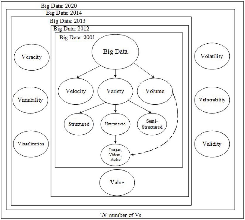
Figure 2 Evolving of big image/video data processing.
Unstructured data, which primarily consists of images and videos, accounts for 80% of all data in the world [16]. Millions of CCTV cameras in affluent countries like the UK record billions of videos each year [17]. The need for storing and searching has expanded significantly as a result of the billions of videos that must be stored and processed. Images and videos are classified as unstructured data by ‘Big Data’ technologies, and the relationship between Image Processing and Video Processing is demonstrated in Figure 2. Big Image/Video Data Processing is the term for this. Many technological issues, like as compression, storage, transmission, analysis, and recognition, that were previously unsolvable with existing technologies can now be addressed [18–21].
Manufacturing, Fraud Detection, Healthcare, Transportation Services, Banking Sector, Media, Communication, and Insurance Services are just a few of the industries where BigData is used. Diseases such as genomics, tumours, chronic obstructive pulmonary disease (COPD), and cancer can be predicted, diagnosed, and monitored in the healthcare system [22, 23]. Transportation services play a significant part in the development of smart cities by planning routes, managing revenue, controlling traffic, and giving travel information to city residents [24]. Analyzing client feedback, shopping behaviours, and finding market regions guide to a superior decision-making process in the field of e-Commerce [25]. Analysis of client behaviour helps a reduction in insurance and banking sector risks [26] with the use of smart devices with GPS functionality and social media.
Map-Reduce: Map-Reduce is a programming technique for processing large amounts of data that uses data from HDFS [27, 28] or the Local File System (LFS).There are two steps to it: the map phase and the reduction phase. The map phase employs the mapper function, which accepts input data in the form of a series of key, value pairs and returns data in the same format. Reducer, which is also a function, will merge the intermediate key, value pairs; this phase is known as the reduce phase.
2 Methodology
In the proposed method, a total of 5 Map-Reduce Jobs: Job-0 to Job-4 are used for the JPEG compression and decompression process. Here, Job-0 is used for convert the images into Sequence files. The Job-1 then receives the Sequence files, applies the JPEG compression and provides the compressed images. Job-2 is used to calculate the compression ratio. The Job-3 receives the compressed files and applies the JPEG decompression. Finally, the Job-4 is used for calculating the Average PSNR (APSNR). The block diagram for this entire process is shown in Figure 3 and the detailed description is given after that.
Job-0: Converting into sequence file:
| Job0: | Mapper | Reducer | |||
| Input | Output | Shuffle and Sort | Input | Output | |
| Creating Sequence Files | Folder, Image Files | FileName, Pixels value of the image | All file names are sorted based on image file names | FileName, Pixels value of the image | Seq.File-1 Seq.File-2 Seq.File-w |
The specified image dataset is initially saved in the local file system (LFS). Figure 4 depicts the Job-0 functionality. The mapper accepts images with any extension (jpg/png/tif…) as input and outputs a key, value pair. If the image is a color image, all three channels i.e. Red, Green, and Blue pixels, are kept as part of the pair. All of these are the inputs for shuffle and sort, and they will all be sorted by key. This sorted data is now fed into the reducer, which will turn it into sequence files. The number of key, value pairs in each sequence file is determined by the software’s maximum sequence file size.
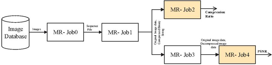
Figure 3 MR Paradigm block diagram of the proposed system. Both input and output for each job are displayed, and performance measures values are calculated.
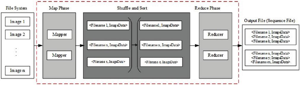
Figure 4 Outline of Map-Reduce Job-0. It is used to convert the given images into sequence files.
Job-1: JPEG compression of image to Binary String
| Job1: | Mapper | Reducer | |||
| Input | Output | Shuffle and Sort | Input | Output | |
| Compression | FileName, Pixels value of the image | FileName, [Original Image, Compressed binary string] | All file names are sorted based on image file names | FileName, [Original image, Compressed binary string] | FileName, [Original Image, Compressed Binary String] |
The mapper accepts the unbundled data as the input i.e., FileName, Pixels value of the image. If the image is in color, the mapper will transform it to grayscale. The JPEG compression given in Algorithm-1 is applied on the image data and converted into compressed binary string. The output of the Mapper is FileName, Compressed binary string. Now, this FileName, Compressed binary string is then shuffled and sorted and stored. The Job-1 functionality is shown in Figure 5. Here in Job-1 the reducer is an identity reducer.
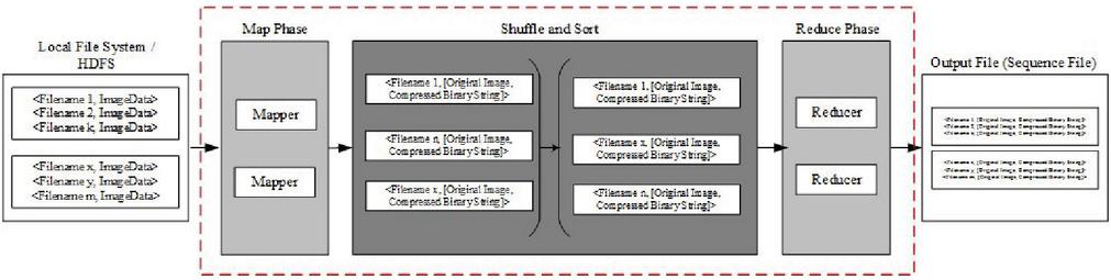
Figure 5 Outline of Map-Reduce Job-1. It is used to compress the whole image data.
Job-2: Calculating Compression Ratio
| Job2: | Mapper | Reducer | |||
| Input | Output | Shuffle and Sort | Input | Output | |
| Average Compression Ratio | FileName, [Original image, Compressed binary string] | Compression Ratio, Average Compression Ratio for m,m…m | All file names are sorted based on image file names | Compression Ratio, Average Compression Ratio for m,m…m | Average Compression Ratio, Result |
The Mapper considers each key value pair. To find the compression ratio for each image the size of the original image and the length of the binary string is found. Then (RC8)/Length of string is used as the measure for compression ratio. The mapper takes the average of all the key-value pairs that it has access to and outputs Compression Ratio, (Average compression ratio for m,m…m) where m,m…m are the various workers. The reducers then takes Compression Ratio, (Average Compression Ratio for m,m…m) as inputs for n workers and calculates the global compression ratio by taking the average of it to output Compression Ratio, Result. Job-2 functionality is shown in Figure 6.
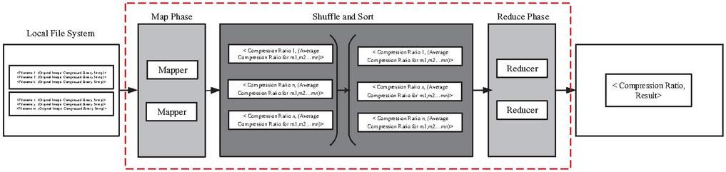
Figure 6 Outline of Map-Reduce Job-2. It is used to calculate the average compression ratio.
Job-3: Decompression
| Job3: | Mapper | Reducer | |||
| Input | Output | Shuffle and Sort | Input | Output | |
| Decompression | FileName, [Original image, Compressed binary string] | FileName, Original image, Decompressed image | All file names are sorted based on image file names | FileName, Original image, Decompressed image | FileName, Original image, Decompressed image |
The Mapper takes the output from Job-1 as the input i.e FileName, [Original image, Compressed binary String]. Using JPEG decompression as in algorithm-2, Job-3 converts all the binary string back to decompressed image of the same size. The output of the Mapper is FileName, [Original image, Decompressed image]. Now, this FileName, [Original image, Decompressed image] is then shuffled and sorted and stored in LFS. The Job-3 functionality is shown in Figure 7.
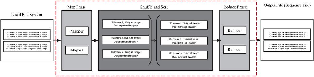
Figure 7 Outline of Map-Reduce Job-3. It is used to decompress the image data.
Job-4: Average PSNR
| Job4: | Mapper | Reducer | |||
| Input | Output | Shuffle and Sort | Input | Output | |
| Average PSNR | FileName, Original image, Decompressed image | PSNR, Average PSNR for m,m…m | All file names are sorted based on PSNR value | PSNR, Average PSNR for m,m…m | APSNR, Result |
The Mapper considers each key value pair. To find the PSNR for each image, the size of the original image and the length of the binary string is calculated which are used to calculate Mean Square Error (MSE) in turn the Peak Signal to Noise Ratio (PSNR). The mapper takes the average of all the key-value pairs that it has access to and outputs PSNR, (Average PSNR for m,m…m) where m,m…m are the various workers. The reducers the takes PSNR, (Average PSNR for m,m…m) as inputs for n workers and calculates the average PSNR to output PSNR, Result for the dataset. Job-4 functionality is show in Figure 8.
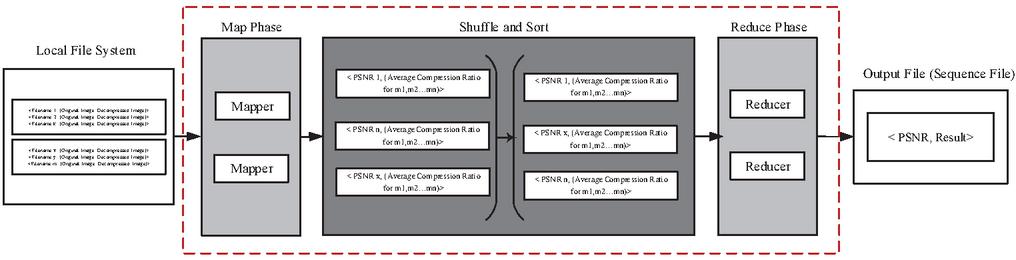
Figure 8 Outline of Map-Reduce Job-4. It is used to calculate average PSNR value.
The JPEG version that is used in this paper is lossy compression applied on gray images. The compression and decompression process in JPEG is explained in detail with the help of Algorithm-1 and Algorithm-2 respectively.
Algorithm-1: JPEG Compression Algorithm
1. Divide the images into blocks of size 88. If the image cannot be divided into 88 blocks, padding (0 padding at the right side and/or at the bottom of the image) is done.
2. For Each 88 block, perform the following steps:
a. In the 88 block, the pixel levels are shifted by -128 intensity levels.
b. DCT is applied on the shifted subimage to get the corresponding DCT coefficients.
c. The DCT coefficients are then divided by the luminance quantization (or normalization) matrix Z, given in Figure 9 and the value is rounded off to the nearest Integer. The scaling of this normalization matrix allows to select the “quality” of JPEG compressions.
d. The resultant matrix obtained is reordered into a 1-D coefficient sequence using the zigzag ordering pattern given in the Figure 10.
e. The reordered coefficient sequence begins with DC coefficient with the remaining 63 values as AC coefficients.
f. In the 1-D coefficient sequence, the AC coefficients containing 0s at the tail are replaced with the EOB which denotes end-of-block. If the AC coefficients contain non-zero values at the last position of the 1-D array, the array is not changed. Note that, a special EOB Huffman code word is provided to indicate that the remaining coefficients in a reordered sequence are 0s.
g. These 1-D coefficients are encoded using the [Appendix-Table A1], [Appendix-Table A2] and [Appendix-Table A3] given in Appendix as:
i. The reordered coefficient sequence begins with a DC coefficient with the remaining 63 values are AC coefficients.
ii. For the DC coefficient, the difference between the current DC coefficient and that of the previously encoded subimage is computed. For the DC coefficient whose previous encoded subimage doesn’t exist, zero is assumed as the previous value for computing the difference.
iii. The resulting difference is checked for which DC difference category it lies in [Appendix-Table A1]. The correct base code for the category difference is selected, N bit code, in accordance with the default Huffman difference code of [Appendix-Table A2], while the overall length of a fully encoded for that category coefficient is L bits. The difference value’s least significant bits (LSBs) must be used to construct the remaining (L-N) bits. An additional K bits are required for a general DC difference category (say, category K), and are computed as either the LSBs of the positive difference or the LSBs of the negative difference minus 1.
iv. The reordered array’s nonzero AC coefficients are coded similarly from [Appendix-Table A1] and [Appendix-Table A3]. Although no difference must be computed for AC coefficients, each default AC Huffman code word is determined by the number of zero-valued coefficients preceding the nonzero coefficient to be coded and the magnitude category of the nonzero coefficient using [Appendix-Table A1]. Based on these pairs, the code word is formed from [Appendix-Table A3]. The remaining steps are similar to the DC coefficient code computation.
v. The encoding is continued until either an EOB is encountered or all 64 values are encoded. Note that, if the AC coefficient value is ‘0’, then there is no Huffman code for this.
h. The Encoding of the 88 is done and a binary string of zeros and ones is obtained.
3. The whole bit pattern obtained for all 88 blocks, the result is stored which is the compressed version of the image.
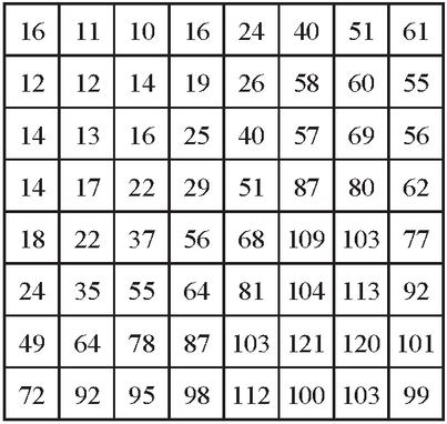
Figure 9 Luminance Quantization ‘or’ normalizing matrix used for JPEG compression.
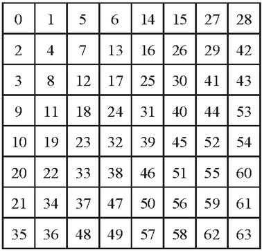
Figure 10 Zigzag ordering/sequence used in JPEG compression.
Algorithm-2: JPEG Decompression Algorithm
1. The Encoded binary string is read bit by bit to check for the corresponding value for the decoding purpose. The decoding process is done so as to obtain the 64 elements using which the 88 block is obtained.
2. First, the DC value is obtained by checking the Binary string for the binary code present in [Appendix-Table A2].
3. The obtained binary code will give the length of the DC encoded value using which the remaining code can be obtained. The Remaining code is then used to obtain the value for the encoded value by using the reverse mapping. (Reverse mapping is done by using the remaining bits to determine the position of the encoded value where the values are sorted in the ascending order as per Range column in [Appendix-Table A1].) Using this, the difference value is obtained which is further added to the previously decoded DC coefficient or the assumed value for the first DC coefficient for the string.
4. The binary encoded string is then decoded to obtain the remaining 63 AC coefficients.
5. For AC coefficients, the decoding is similar to DC coefficients where the code is read and matched with the codes in the [Appendix-Table A3] to obtain the Run, category and Length for the encoded value. Using Run value, the zeros are appended into the array same as the value of Run. The Category value is used to determine the range of values in [Appendix-Table A1]. Using Length, the index of the value for the encoded value is obtained by taking into consideration the Length and removing the MSBs matched with the code in [Appendix-Table A3]. With the help of the decimal value of the bits, the encoded value can be retrieved from the binary string.
6. The AC coefficients are determined until either a total of 64 elements obtained (1 DC coefficient and 63 AC coefficient) or an EOB is encountered in which case the remaining values are filled with zeros till the end of the array. This will gives the 1-D coefficients of length 64.
7. Using the 1-D coefficients obtained, the inverse zigzag operation is applied to obtain a 88 block which is shown in Figure 10.
8. The Resultant matrix is then multiplied with the Luminance matrix given in Figure 9, giving the DCT coefficients of the original subimage.
9. The values of the image are then obtained using the Inverse Discrete Cosine Transform operation.
10. In the 88 subimage block, the pixel levels are shifted by 128 intensity levels.
11. Steps (2)–(10) are repeated until the whole binary string is read which is stored in the correct original image position to give the Image close to the Original Image.
3 Results and Discussions
In this section, the results of compression and decompression using JPEG on different image datasets using different number of workers in MR paradigm are given. The two image datasets: STex textures and Corel-5000 are considered and preprocessed them to get more than one million images to test the performance of the MR paradigm with different number of workers.
STex Image Dataset: For creating the image dataset, the standard STex image dataset containing 476 512512 images is used. Each image is then divided into 256 subimages with size of each being 3232 thus giving 121,856 images. These 121,856 images were used with different replication factors to create all the datasets used for the experimentation. Total number of images in each dataset is given in Table 1. All these datasets are considered individually to test both the compression methods by using the number of workers.
Table 1 Different image datasets with their sizes used in this work
| S.No. | Dataset Creation Method | Number of Images |
| 1 | First 25,000 of row 4 | 25,000 |
| 2 | First 50,000 of row 4 | 50,000 |
| 3 | First 75,000 of row 4 | 75,000 |
| 4 | All 476 Textures made into 3232 | 121,856 |
| 5 | 5 Times of 4 | 609,280 |
| 6 | 9 Times of 4 | 1,096,704 |
| 7 | Corel-5000 | 5,000 |
Corel-5000 Image Dataset: Also, JPEG compression and decompression is executed on the Corel-5K image dataset. It consists of 5,000 images and this dataset is generally used to test content based image retrieval (CBIR) algorithms. In this paper, for compression and decompression the sane image dataset is used.
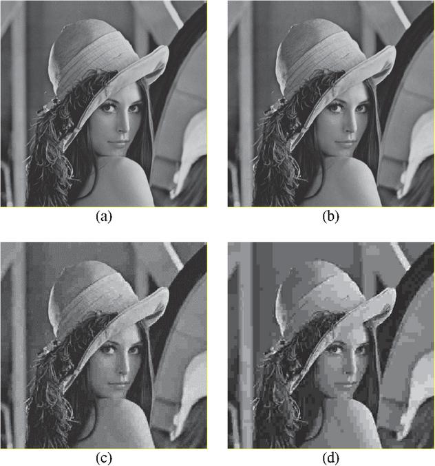
Figure 11 JPEG Compression Results for Lenna Image (a) Original image (b) Decompressed image with Quality Factor 1 (c) Decompressed image with Quality Factor 5 (d) Decompressed image with Quality Factor 10.
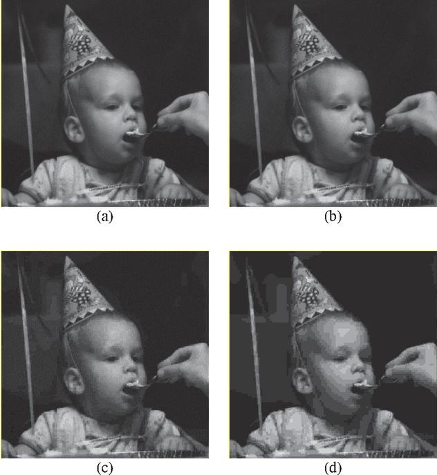
Figure 12 JPEG Compression Results for Child Image (a) Original image (b) Decompressed image with Quality Factor 1 (c) Decompressed image with Quality Factor 5 (d) Decompressed image with Quality Factor 10.
To show the visual comparison of the images before compression and after decompression, the results JPEG on Lenna image [29], Child image [29] and Texture image [30] are shown in Figures 11, 12 and 13 respectively. The statistical comparisons are given in Table 2.
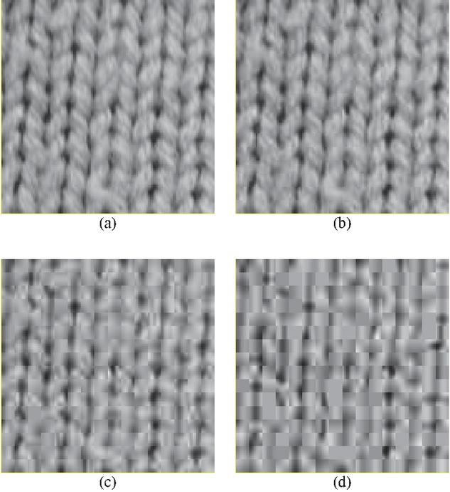
Figure 13 JPEG Compression Results for Texture Image (a) Original image (b) Decompressed image with Quality Factor 1 (c) Decompressed image with Quality Factor 5 (d) Decompressed image with Quality Factor 10.
Performance measures for analyzing the compression technique: Compression Ratio: To measure the performance of this compression process, ‘compression ratio’ is calculated using the Equation (5).
| (5) |
where ‘ob’ is the number of bits needed originally to represent an image as a 2-D array of intensity values and ‘cb’ is the number of bits needed to represent the image in compressed form.
Average Compression Ratio (ACR): The average compression ratio of all the images considered can be calculated by using the Equation (6).
| (6) |
Table 2 JPEG results for the three images considered with the three quality factors 1, 5 and 10
| Compression Ratio | RMSE | PSNR | |||||||
| QF:1 | QF:5 | QF:10 | QF:1 | QF:5 | QF:10 | QF:1 | QF:5 | QF:10 | |
| Lenna | 13.52 | 34.96 | 48.39 | 3.83 | 7.34 | 10.68 | 36.47 | 30.82 | 27.56 |
| Child | 25.18 | 49.13 | 59.73 | 2.43 | 4.78 | 7.27 | 40.41 | 34.54 | 30.90 |
| Texture | 7.63 | 19.46 | 30.35 | 4.36 | 9.87 | 14.52 | 35.34 | 28.25 | 24.89 |
Mean Square Error (MSE): The MSE is a measure of the differences between image pixel values after decompression and the original pixel values of the image before compression. The value of MSE depends on the size of the image. The value of MSE decreases with increase in the size of the image. The value of MSE can be calculated using Equation (7).
| (7) |
where is the original image and is the decompressed image, m and n are the size of the image, mn is the size of the image.
Average Peak Signal to Noise Ratio (APSNR): PSNR is most commonly used to measure the quality of reconstruction. The relation between MSE and PSNR is that, as the value of MSE decreases, the value of PSNR increases. It can also be said that the value of PSNR increases with the increase in the size of the image (as MSE decreases with size). Also, it can also be deduced that the value of PSNR increases with the increase in the Maximum value for the given number of bits required to represent the image. At any time, the minimum value of PSNR is 0 and maximum value of PSNR is infinity. The value of PSNR and APSNR can be calculated using the Equations (8) and (9) respectively.
| (8) |
Here, is the maximum possible pixel value of the image. This is 255 when the pixels are represented using 8 bits per sample.
| (9) |
where, n is the number of images in the dataset.
The JPEG compression technique is applied on the image datasets given in Table 1 by using the single system, 2 workers with MR and 4 workers with MR paradigm. The performance measures and execution time for the datasets using JPEG are given in Tables 5 to 5. Based on these results, graphs are drawn to show the comparison of these executions.
Table 3 Single system; no map-reduce
| Statistics of the Data | Time to complete the Job in Sec. | |||||||||
| Number | Size of Images – | Size of Images – | Avg | Avg | Total | |||||
| S.No. | of Images | Before Compression (Bits) | After Compression (Bits) | CR | PSNR | Compression | ACR | Decompression | APSNR | Time |
| 1 | 25,000 | 204,800,000 | 28,983,136 | 8.82 | 33.26 | 1030.54 | 0.16 | 664.18 | 1.01 | 1695.89 |
| 2 | 50,000 | 409,600,000 | 54,713,474 | 9.70 | 33.88 | 1986.87 | 0.27 | 1256.90 | 1.88 | 3245.92 |
| 3 | 75,000 | 614,400,000 | 77,668,922 | 10.74 | 34.36 | 2756.99 | 0.36 | 1839.68 | 2.77 | 4599.79 |
| 4 | 121,856 | 998,244,352 | 121,271,603 | 11.18 | 34.57 | 4304.96 | 0.52 | 2856.46 | 4.44 | 7166.38 |
| 5 | Corel-5000 | 948,761,664 | 132,575,602 | 7.92 | 30.97 | 4634.76 | 0.03 | 2623.32 | 0.68 | 7258.80 |
Table 4 Map-reduce; 2-workers
| Statistics of the Data | Time in Sec. | ||||||||||
| Number | Size of Images – | Size of Images – | Avg | Avg | Total | ||||||
| S.No. | of Images | Before Compression (Bits) | After Compression (Bits) | CR | PSNR | Job-0 | Job-1 | Job-2 | Job-3 | Job-4 | Time |
| 1 | 25,000 | 204,800,000 | 28,983,136 | 8.82 | 33.26 | 79.74 | 530.41 | 15.37 | 358.73 | 16.48 | 1000.73 |
| 2 | 50,000 | 409,600,000 | 54,713,474 | 9.70 | 33.88 | 116.89 | 1034.51 | 31.12 | 712.56 | 32.08 | 1927.17 |
| 3 | 75,000 | 614,400,000 | 77,668,922 | 10.74 | 34.36 | 135.39 | 1439.33 | 42.83 | 1025.63 | 45.42 | 2688.60 |
| 4 | 121,856 | 998,244,352 | 121,271,603 | 11.18 | 34.57 | 144.08 | 2251.47 | 68.33 | 1608.60 | 71.61 | 4144.09 |
| 5 | Corel-5000 | 948,761,664 | 132,575,602 | 7.92 | 30.97 | 83.28 | 2283.66 | 5.74 | 1197.72 | 5.70 | 3576.11 |
Table 5 Map-reduce; 4-workers
| Statistics of the Data | Time in Sec. | ||||||||||
| Number | Size of Images – | Size of Images – | Avg | Avg | Total | ||||||
| S.No. | of Images | Before Compression (Bits) | After Compression (Bits) | CR | PSNR | Job-0 | Job-1 | Job-2 | Job-3 | Job-4 | Time |
| 1 | 25,000 | 204,800,000 | 28,983,136 | 8.82 | 33.26 | 52.89 | 292.16 | 11.43 | 194.61 | 10.97 | 562.06 |
| 2 | 50,000 | 409,600,000 | 54,713,474 | 9.70 | 33.88 | 78.78 | 559.65 | 18.91 | 381.28 | 19.87 | 1058.49 |
| 3 | 75,000 | 614,400,000 | 77,668,922 | 10.74 | 34.36 | 94.77 | 783.79 | 27.08 | 533.52 | 27.38 | 1466.53 |
| 4 | 121,856 | 998,244,352 | 121,271,603 | 11.18 | 34.57 | 162.00 | 1232.78 | 40.95 | 913.67 | 43.11 | 2392.51 |
| 5 | Corel-5000 | 948,761,664 | 132,575,602 | 7.92 | 30.97 | 78.30 | 1286.37 | 4.50 | 663.43 | 4.83 | 2037.42 |
To show the time comparison for different setups for each of the jobs, the graphs are drawn and are shown in Figures 14 to 18. These figures clearly show that the time to complete with 4 workers is significantly less than with a single system or 2 workers setups. The time advantage achieved is calculated and shown in Table 6.

Figure 14 Time graph for 25,000 Images.
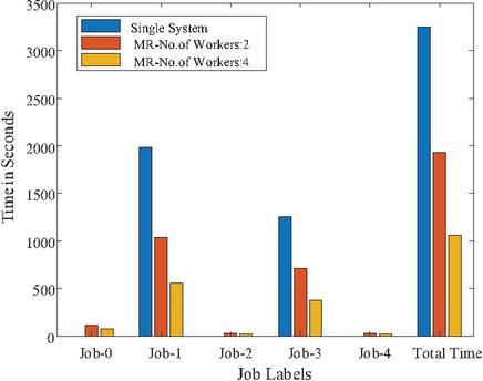
Figure 15 Time graph for 50,000 Images.
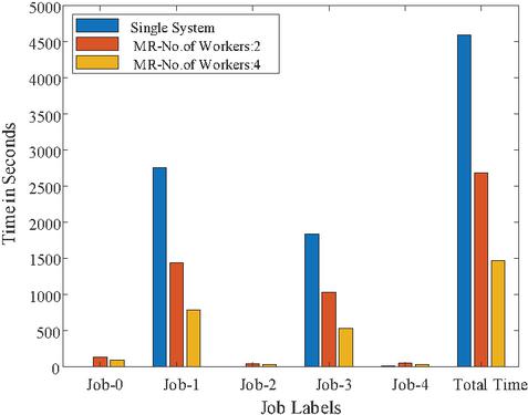
Figure 16 Time graph for 75,000 Images.
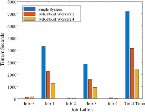
Figure 17 Time graph for 121,856 Images.
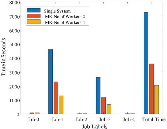
Figure 18 Time graph for Corel-5000 Images.
Table 6 The total amount of time saved for all image datasets considered. The top section of the table displays the time in seconds, while the lower part displays the percentage of time saved with various worker counts
| 25,000 | 50,000 75,000 | 121,856 | Corel-5000 | 609,280 | 1,096,704 | ||
| Single System | 1695.89 | 3245.92 | 4599.79 | 7166.38 | 7258.80 | 21310.41 | 38205.01 |
| MR-No. of Workers: 2 | 1000.73 | 1927.17 | 2688.60 | 4144.09 | 3576.11 | — | — |
| MR-No. of Workers: 4 | 562.06 | 1058.49 | 1466.53 | 2392.51 | 2037.42 | 7010.98 | 12999.34 |
| % of Saved Time: 2 over Single | 41% | 41% | 42% | 42% | 51% | — | — |
| % of Saved Time: 4 over Single | 67% | 67% | 68% | 67% | 72% | 67% | 66% |
| % of Saved Time: 4 over 2 | 44% | 45% | 45% | 42% | 43% | — | — |
In Tables 5, 5 and 5 the results are shown up to 121,856 and for Core-5000 image dataset. But for the other two datasets 609,280 and 1,096,704, the time to complete both compression and decompression takes a lot of time. For these two datasets only JPEG compression is done on single system and 4 workers with MR paradigm. The time comparison for this is shown in Figure 19.
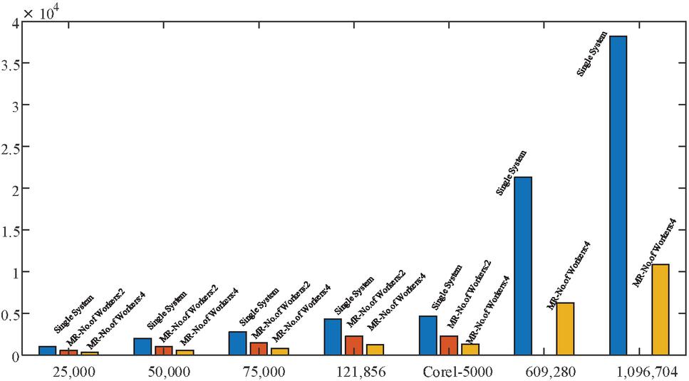
Figure 19 Time graph for 10 Lakh Images.
4 Conclusion and Future Extension
In this paper a technique to handle big image data is shown by successfully compressing as well as decompressing 121,856 images and also compressing more than one million (1,096,704) images with the help of Map-Reduce paradigm. The compressed images size was 12.15% of the original image dataset size by using JPEG compression technique. Since the whole process was executed in distributed environment with four workers, it took 31.82% of the time taken by the single system execution for the complete compression-decompression cycle. Also, when the whole process was executed with two workers, it took 56.79% of the time taken by the single system execution. This paper has proved here that distributed environment can significantly reduce the execution time to handle big image data.
Appendix
Table A1: JPEG coefficient coding categories
| Range | DC Difference Category | AC Category |
| 0 | 0 | N/A |
| -1,1 | 1 | 1 |
| -3,-2,2,3 | 2 | 2 |
| -7,…,-4,4,…,7 | 3 | 3 |
| -15,…,-8,8,…,15 | 4 | 4 |
| -31,…,-16,16,…,31 | 5 | 5 |
| -63,…,-32,32,…,63 | 6 | 6 |
| -127,…,-64,64,…,127 | 7 | 7 |
| -255,…,-128,128,…,255 | 8 | 8 |
| -511,…,-256,256,…,511 | 9 | 9 |
| -1023,…,-512,512,…,1023 | A | A |
| -2047,…,-1024,1024,…,2047 | B | B |
| -4095,…,-2048,2048,…,4095 | C | C |
| -8191,…,-4096,4096,…,8191 | D | D |
| -16383,…,-8192,8192,…,16383 | E | E |
| -32767,…,-16384,16384,…,32767 | F | N/A |
Table A2: JPEG default DC Code (luminance)
| Category | Base Code | Length |
| 0 | 010 | 3 |
| 1 | 011 | 4 |
| 2 | 100 | 5 |
| 3 | 00 | 5 |
| 4 | 101 | 7 |
| 5 | 110 | 8 |
| 6 | 1110 | 10 |
| 7 | 11110 | 12 |
| 8 | 111110 | 14 |
| 9 | 1111110 | 16 |
| A | 11111110 | 18 |
| B | 111111110 | 20 |
Table A3: JPEG default AC Code (luminance)
| Run/ | Base | Run/ | Base | Run/ | Base | |||
| Category | Code | Length | Run/ | Code | Category | Code | Length | |
| 0/0 | 1010 (EOB) | 4 | 5/4 | 1111111110100000 | 20 | A/8 | 1111111111001110 | 24 |
| 0/1 | 00 | 3 | 5/5 | 1111111110100001 | 21 | A/9 | 1111111111001111 | 25 |
| 0/2 | 01 | 4 | 5/6 | 1111111110100010 | 22 | A/A | 1111111111010000 | 26 |
| 0/3 | 100 | 6 | 5/7 | 1111111110100011 | 23 | B/1 | 111111010 | 10 |
| 0/4 | 1011 | 8 | 5/8 | 1111111110100100 | 24 | B/2 | 1111111111010001 | 18 |
| 0/5 | 11010 | 10 | 5/9 | 1111111110100101 | 25 | B/3 | 1111111111010010 | 19 |
| 0/6 | 111000 | 12 | 5/A | 1111111110100110 | 26 | B/4 | 1111111111010011 | 20 |
| 0/7 | 1111000 | 14 | 6/1 | 1111011 | 8 | B/5 | 1111111111010100 | 21 |
| 0/8 | 1111110110 | 18 | 6/2 | 11111111000 | 13 | B/6 | 1111111111010101 | 22 |
| 0/9 | 1111111110000010 | 25 | 6/3 | 1111111110100111 | 19 | B/7 | 1111111111010110 | 23 |
| 0/A | 1111111110000011 | 26 | 6/4 | 1111111110101000 | 20 | B/8 | 1111111111010111 | 24 |
| 1/1 | 1100 | 5 | 6/5 | 1111111110101001 | 21 | B/9 | 1111111111011000 | 25 |
| 1/2 | 111001 | 8 | 6/6 | 1111111110101010 | 22 | B/A | 1111111111011001 | 26 |
| 1/3 | 1111001 | 10 | 6/7 | 1111111110101011 | 23 | C/1 | 1111111010 | 11 |
| 1/4 | 111110110 | 13 | 6/8 | 1111111110101100 | 24 | C/2 | 1111111111011010 | 18 |
| 1/5 | 11111110110 | 16 | 6/9 | 1111111110101101 | 25 | C/3 | 1111111111011011 | 19 |
| 1/6 | 1111111110000100 | 22 | 6/A | 1111111110101110 | 26 | C/4 | 1111111111011100 | 20 |
| 1/7 | 1111111110000101 | 23 | 7/1 | 11111001 | 9 | C/5 | 1111111111011101 | 21 |
| 1/8 | 1111111110000110 | 24 | 7/2 | 11111111001 | 13 | C/6 | 1111111111011110 | 22 |
| 1/9 | 1111111110000111 | 25 | 7/3 | 1111111110101111 | 19 | C/7 | 1111111111011111 | 23 |
| 1/A | 1111111110001000 | 26 | 7/4 | 1111111110110000 | 20 | C/8 | 1111111111100000 | 24 |
| 2/1 | 11011 | 6 | 7/5 | 1111111110110001 | 21 | C/9 | 1111111111100001 | 25 |
| 2/2 | 11111000 | 10 | 7/6 | 1111111110110010 | 22 | C/A | 1111111111100010 | 26 |
| 2/3 | 1111110111 | 13 | 7/7 | 1111111110110011 | 23 | D/1 | 11111111010 | 12 |
| 2/4 | 1111111110001001 | 20 | 7/8 | 1111111110110100 | 24 | D/2 | 1111111111100011 | 18 |
| 2/5 | 1111111110001010 | 21 | 7/9 | 1111111110110101 | 25 | D/3 | 1111111111100100 | 19 |
| 2/6 | 1111111110001011 | 22 | 7/A | 1111111110110110 | 26 | D/4 | 1111111111100101 | 20 |
| 2/7 | 1111111110001100 | 23 | 8/1 | 11111010 | 9 | D/5 | 1111111111100110 | 21 |
| 2/8 | 1111111110001101 | 24 | 8/2 | 111111111000000 | 17 | D/6 | 1111111111100111 | 22 |
| 2/9 | 1111111110001110 | 25 | 8/3 | 1111111110110111 | 19 | D/7 | 1111111111101000 | 23 |
| 2/A | 1111111110001111 | 26 | 8/4 | 1111111110111000 | 20 | D/8 | 1111111111101001 | 24 |
| 3/1 | 111010 | 7 | 8/5 | 1111111110111001 | 21 | D/9 | 1111111111101010 | 25 |
| 3/2 | 111110111 | 11 | 8/6 | 1111111110111010 | 22 | D/A | 1111111111101011 | 26 |
| 3/3 | 11111110111 | 14 | 8/7 | 1111111110111011 | 23 | E/1 | 111111110110 | 13 |
| 3/4 | 1111111110010000 | 20 | 8/8 | 1111111110111100 | 24 | E/2 | 1111111111101100 | 18 |
| 3/5 | 1111111110010001 | 21 | 8/9 | 1111111110111101 | 25 | E/3 | 1111111111101101 | 19 |
| 3/6 | 1111111110010010 | 22 | 8/A | 1111111110111110 | 26 | E/4 | 1111111111101110 | 20 |
| 3/7 | 1111111110010011 | 23 | 9/1 | 111111000 | 10 | E/5 | 1111111111101111 | 21 |
| 3/8 | 1111111110010100 | 24 | 9/2 | 1111111110111111 | 18 | E/6 | 1111111111110000 | 22 |
| 3/9 | 1111111110010101 | 25 | 9/3 | 1111111111000000 | 19 | E/7 | 1111111111110001 | 23 |
| 3/A | 1111111110010110 | 26 | 9/4 | 1111111111000001 | 20 | E/8 | 1111111111110010 | 24 |
| 4/1 | 111011 | 7 | 9/5 | 1111111111000010 | 21 | E/9 | 1111111111110011 | 25 |
| 4/2 | 1111111000 | 12 | 9/6 | 1111111111000011 | 22 | E/A | 1111111111110100 | 26 |
| 4/3 | 1111111110010111 | 19 | 9/7 | 1111111111000100 | 23 | F/0 | 111111110111 | 12 |
| 4/4 | 1111111110011000 | 20 | 9/8 | 1111111111000101 | 24 | F/1 | 1111111111110101 | 17 |
| 4/5 | 1111111110011001 | 21 | 9/9 | 1111111111000110 | 25 | F/2 | 1111111111110110 | 18 |
| 4/6 | 1111111110011010 | 22 | 9/A | 1111111111000111 | 26 | F/3 | 1111111111110111 | 19 |
| 4/7 | 1111111110011011 | 23 | A/1 | 111111001 | 10 | F/4 | 1111111111111000 | 20 |
| 4/8 | 1111111110011100 | 24 | A/2 | 1111111111001000 | 18 | F/5 | 1111111111111001 | 21 |
| 4/9 | 1111111110011101 | 25 | A/3 | 1111111111001001 | 19 | F/6 | 1111111111111010 | 22 |
| 4/A | 1111111110011110 | 26 | A/4 | 1111111111001010 | 20 | F/7 | 1111111111111011 | 23 |
| 5/1 | 1111010 | 8 | A/5 | 1111111111001011 | 21 | F/8 | 1111111111111100 | 24 |
| 5/2 | 1111111001 | 12 | A/6 | 1111111111001100 | 22 | F/9 | 1111111111111101 | 25 |
| 5/3 | 1111111110011111 | 19 | A/7 | 1111111111001101 | 23 | F/A | 1111111111111110 | 26 |
References
[1] Rafel C. Gonzalez and Richard E. Woods, “Digital Image Processing”, 3rd Edition, Person.
[2] Kazuhiro Kobayashi and Qiu Chen Content-Based Image Retrieval Using Features in Spatial and Frequency Domains, ICSIIT 2015, CCIS 516, pp. 269–277, 2015. DOI: https://doi.org/10.1007/978-3-662-46742-8\_25
[3] J. A. Stuchi et al., “Improving image classification with frequency domain layers for feature extraction,” 2017 IEEE 27th International Workshop on Machine Learning for Signal Processing (MLSP), 2017, pp. 1–6, doi: https://doi.org/10.1109/MLSP.2017.8168168.
[4] I. H. Witten, R. M. Neal, and J. G. Cleary, “Arithmetic coding for data compression,” Communications of the ACM, vol. 30, no. 6, pp. 520–540, 1987.
[5] S. Golomb, “Run-length encodings (Corresp.),” IEEE Trans. on information theory, vol. 12, no. 3, pp. 399–401, 1966.
[6] D. A. Huffman, “A method for the construction of minimum redundancy codes,” Proceedings of the IRE, vol. 40, no. 9, pp. 1098–1101, 1952.
[7] H. Andrews and W. Pratt, “Fourier transform coding of images,” in Proc. Hawaii Int. Conf. System Sciences, 1968, pp. 677–679.
[8] W. K. Pratt, J. Kane, and H. C. Andrews, “Hadamard transform image coding,” Proceedings of the IEEE, vol. 57, no. 1, pp. 58–68, 1969.
[9] N. Ahmed, T. Natarajan, and K. R. Rao, “Discrete cosine transform,” IEEE Trans. on Computers, vol. 100, no. 1, pp. 90–93, 1974.
[10] C. Harrison, “Experiments with linear prediction in television,” Bell System Technical Journal, vol. 31, no. 4, pp. 764–783, 1952.
[11] C. Christopoulos, A. Skodras, and T. Ebrahimi, “The JPEG2000 still image coding system: an overview,” IEEE trans. on consumer electronics, vol. 46, no. 4, pp. 1103–1127, 2000.
[12] D. Taubman, “High performance scalable image compression with EBCOT,” IEEE Trans. on image processing, vol. 9, no. 7, pp. 1158–1170, 2000.
[13] Mayer-Schönberger Viktor, and Kenneth Cukier. Big data: A revolution that will transform how we live, work, and think. Houghton Mifflin Harcourt, 2013.
[14] Uddin Muhammad Fahim, and Navarun Gupta. “Seven V’s of Big Data understanding Big Data to extract value.” In Proceedings of the 2014 zone 1 conference of the American Society for Engineering Education, pp. 1–5. IEEE, 2014.
[15] The 42V’s of BIG Data and Data Science, https://www.kdnuggets.com/2017/04/42-vs-big-data-data-science.html
[16] Fritz Venter, Andrew Stein (2012) Analytics: Driving better business decisions. http://analytics-magazine.org/images-a-videos-really-big-data/
[17] Mark Sugrue (2015) CCTV- the challenge of sifting through Big Data. https://www.engineersireland.ie/Engineers-Journal/Technology/cctv-the-challenge-of-sifting-through-big-data
[18] Wang Weining., Weijian Zhao, Chengjia Cai, Jiexiong Huang, Xiangmin Xu, and Lei Li. “An efficient image aesthetic analysis system using Hadoop.” Signal Processing: Image Communication 39 (2015): 499–508.
[19] Lin Yuanqing., Fengjun Lv, Shenghuo Zhu, Ming Yang, Timothee Cour, Kai Yu, Liangliang Cao, and Thomas Huang. “Large-scale image classification: fast feature extraction and svm training.” In CVPR 2011, pp. 1689–1696. IEEE, 2011.
[20] Zhang Shiliang., Ming Yang, Xiaoyu Wang, Yuanqing Lin, and Qi Tian. “Semantic-aware co-indexing for image retrieval.” In Proceedings of the IEEE international conference on computer vision, pp. 1673–1680. 2013.
[21] Dong Le, Zhiyu Lin, Yan Liang, Ling He, Ning Zhang, Qi Chen, Xiaochun Cao, and Ebroul Izquierdo. “A hierarchical distributed processing framework for big image data.” IEEE Transactions on Big Data 2, no. 4 (2016): 297–309.
[22] ProjectPro. Healthcare applications of Hadoop and Big data. https://www.dezyre.com/article/5-healthcare-applications-of-hadoop-and-big-data/85
[23] Koppad Shaila H., and Anupamma Kumar. “Application of big data analytics in healthcare system to predict COPD.” In 2016 International Conference on Circuit, Power and Computing Technologies (ICCPCT), pp. 1–5. IEEE, 2016.
[24] Chen Mao., Zhong Xugang, Wang Guansen, and Ma Jianxiao. “A preliminary discussion on the application of big data in urban residents travel guidance.” In 2015 International Conference on Intelligent Transportation, Big Data and Smart City, pp. 47–50. IEEE, 2015.
[25] Im Hyeongsoon., Bonghee Hong, Seungwoo Jeon, and Jaegi Hong. “Bigdata analytics on CCTV images for collecting traffic information.” In 2016 International Conference on Big Data and Smart Computing (BigComp), pp. 525–528. IEEE, 2016.
[26] Applications of Big Data Drive Industries. https://www.simplilearn.com/tutorials/big-data-tutorial/big-data-applications
[27] Turkington G., (2013). Hadoop Beginner’s Guide. Packt Publishing Ltd.
[28] Perera S., (2013). Hadoop MapReduce Cookbook. Packt Publishing Ltd.
[29] Gonzalez, R.C., Woods, R.E.: http://www.imageprocessingplace.com/ (Accessed 27 August 2021).
[30] Kwitt, R., Peter, M.: Salzburg Texture Image Dataset, http://www.wavelab.at/sources/STex/, (Accessed 27 August 2021).
Biographies
U. S. N. Raju received the B.E. (CSE) degree from Bangalore University in 1998, M. Tech. (Software Engineering) from JNT University in 2002 and Ph.D.(CSE) from JNT University Kakinada in 2010. He worked in industry for two years and then in academics for 18 years. Presently he is working in department of Computer Science and Engineering at National Institute of Technology Warangal, Telangana State, India since 9 years. He is a senior member of IEEE and life member of ISTE, CSI, ISCA and IEI. His area of research is Big Image Data Processing and Deep Learning for Computer Vision. He has visited UK, Malaysia, China, Thailand, Taiwan and USA to present his research work.
Hillol Barman received the B.Tech. degree in Information Technology from University College of Science and Technology, University of Calcutta, Kolkata, India in 2019 and is pursuing his M.Tech. in Computer Science and Engineering from NIT Warangal, Telangana, India. His research interests are in the fields of Image Processing, Big Data technologies, Computer Graphics and Artificial Intelligence with an emphasis on image compression and decompression.

Netalkar Rohan Kishor, received the B.E. degree in Computer Engineering from Ramrao Adik Institute of Technology (RAIT), Navi Mumbai, India in 2018 and is pursuing his M.Tech. in Computer Science and Engineering from National Institute of Technology Warangal, Telangana, India. His research interests are in the fields of Image Processing, Big Data technologies with an emphasis on image compression and image retrieval.

Sanjay kumar, received the Bachelor of Computer Applications degree from Anugrah Narayan College,Patna, India in 2018 and is pursuing his MCA from National Institute of Technology Warangal, Telangana, India. His research interests are in the fields of Image Processing, Big Data technologies with an emphasis on image compression and image retrieval.

Hariom Kumar, received the Bachelor of Computer Applications degree from Magadh University, BodhGaya(Bihar) in 2018 and is pursuing his Masters of Computer Application from National Institute of Technology Warangal, Telangana, India. His research interests are in the fields of Image Processing, Big Data technologies with an emphasis on image compression and image retrieval.
Journal of Mobile Multimedia, Vol. 18_6, 1513–1540.
doi: 10.13052/jmm1550-4646.1863
© 2022 River Publishers