Gold-Price Forecasting Method Using Long Short-Term Memory and the Association Rule
Laor Boongasame1, 2, Piboonlit Viriyaphol3, Kriangkrai Tassanavipas4 and Punnarumol Temdee5,*
1Department of Mathematics, Faculty of Science, King Mongkut’s Institute of Technology Ladkrabang, Bangkok 10520, Thailand
2Business Innovation and Investment Laboratory: B2I-Lab, Faculty of Science, King Mongkut’s Institute of Technology Ladkrabang, Bangkok 10520, Thailand
3Gold Research Center, Gold Traders Association, Bangkok, Thailand
4Faculty of Engineering and Technology, Panyapiwat Institute of Management, Nonthaburi 11120, Thailand
5Computer and Communication Engineering for Capacity Building Research Center, School of Information Technology, Mae Fah Luang University, Chiang Rai 57100, Thailand
E-mail: laor.bo@kmitl.ac.th; piboonlit@gmail.com; kriangkraitas@pim.ac.th; punnarumol@mfu.ac.th
*Corresponding Author
Received 13 December 2021; Accepted 31 May 2022; Publication 15 September 2022
Abstract
Since gold prices influence international economic and monetary systems, numerous studies have been conducted to forecast gold prices. Nonetheless, studies employing the linear relationship method usually fail to explain the change in the pattern of the gold price. This study introduces a new paradigm that incorporates association rules and long short-term memory (LSTM) as a nonlinear-based method. For simulation, the proposed method was analyzed with data from Yahoo Finance from January 2010 to December 2020. The association rule was used to choose features relevant to the gold spot (GS) in the US Dollar Index (DXY). The LSTM forecast the gold price with a range of hyperparameter settings. The simulation results showed that the proposed method—the LSTM with GS and DXY, or LSTM-GS-DXY—resulted in low mean absolute percentage error (MAPE) metrics. In addition, the proposed LSTM-GS-DXY system outperformed the simple moving average (SMA), weight moving average (WMA), exponential moving average (EMA), and auto-regressive integrated moving average (ARIMA).
Keywords: LSTM, gold forecasting, association rule, artificial neural network.
1 Introduction
Gold is one of the most important commodities in the world. It traditionally has had a strong impact on international economic and monetary systems. It represents strength, wealth, and political power and symbolizes success and admiration. In finance and investing, gold provides higher competitive returns than other major financial assets. Fluctuations in gold prices can increase the risk of investment; the causes of these fluctuations have numerous influences. Gold prices are positively linked to inflation rates [1]. Thus, the major macroeconomic variables that affect the spot price of gold in the short and long terms are usually reviewed [2]. Consequently, the Federal Reserve System (FED), the West Texas Intermediate (WTI), the Inflation Expectations (INF), the Dow Jones Industrial Average (DJI), and the US Dollar Index (DXY) are all widely used to forecast the gold price [1–3]. The FED is the central bank of the United States central bank that ensures the smooth operation of the US economy and long-term public interest rates [4]. The WTI is a medium, sweet crude oil used as a global benchmark. Benchmarks are relevant in the oil market because they act as price guides for buyers and sellers of crude oil [5].
The DJI is one of the leading corporate and financial news organizations in the world. In addition to its most well-known index, the firm has produced several other market indexes [6]. The USDX indicates the dollar’s value concerning an array of currencies representing most of the United States’ major trading partners. The index began in 1973 with a base of 100; all subsequent values have been determined relative to this base, formed soon after the Bretton Woods Agreement was terminated. As part of this deal, participating countries settled their accounts in US dollars (the reserve currency), which were completely convertible to gold at a rate of $35 per ounce [7]. The euro (EUR), Japanese yen (JPY), Canadian dollar (CAD), British pound (GBP), Swedish krona (SEK), and Swiss franc (CHF) are the six main world currencies currently used to measure the USDX.
Gold-price forecasting establishes a model that can predict prices in the near future in relation to a variable set of features. Hence, it is essential for researchers to extract the features affecting forecasting accuracy. Existing works on gold-price forecasting are divided into two categories—including the linear-based method, using the determined relationships among relevant factors to forecast goal prices [8–12], and the nonlinear-based method, using the stochastic relationships among relevant factors to forecast goal prices [10, 13, 14]. Although the nonlinear-based methods have greater performance than the linear-based methods when forecasting accuracy, these methods generally fail to assess the local optimum because they lack global search capabilities. Consequently, a forecasting method with a searching capability is required to address the local maximum limitations of existing nonlinear-based methods for gold forecasting, such as a deep-learning-based method. For this study, long short-term memory (LSTM), one of the most advanced deep-learning methods widely accepted for sequence learning tasks such as time-series prediction [15], is used to forecast the gold price from macroeconomic variables, including the WTI, DJI, and USDXY. Additionally, the association rule can be used to choose features relevant to the gold price. With associated parameter settings, the forecasting performance of LSTM is shown in mean absolute percentage error (MAPE) metrics for comparison purposes with other existing methods.
The remainder of this paper is organized as follows. Section 2 includes the background and associated works. Section 3 provides the research methodology, findings, and interpretations. Finally, Section 4 concludes with a discussion of future research.
2 Literature Review and Background
This study’s literature review is explored in this section, including gold-price forecasting, association rules, and long-term memory, respectively.
2.1 Gold-Price Forecasting
As previously mentioned, the methods used to forecast gold prices can be classified into two groups according to relationships among factors. First, methods using linear relationships among factors to forecast gold prices, especially the generalized auto-regressive conditional heteroskedasticity (GARCH) method, were widely found to determine gold prices. This is a statistical model used to analyze time-series data; it assumes that the variance of the error term follows an auto-regressive moving average process. For example, Kroner et al. [8] and Tully and Lucey [11] used the GARCH model and its extension called asymmetric power GARCH (AP-GARCH) model, respectively, to forecast gold-price fluctuations. The comparisons in forecasting gold-market volatility among different methods were widely found in the GARCH, threshold ARCH (TARCH), threshold GARCH (TGARCH), and auto-regressive moving average process (ARMA) models. The TARCH model was determined to be the most reliable [12].
Second, gold prices are predicted using methods with nonlinear relationships among factors. The machine-learning-based method known as artificial neural networks (ANNs) was applied generally. For example, Zhou et al. [16] used a back-propagation neural network (BPNN) model to forecast gold prices. Kristjanpoller and Minutolo [9] improved the GARCH technique, and Schmidhuber [15] forecast gold-price changes by using ANN models. Hafezi and Akhavan [14] suggested a new intelligent network with a meta-heuristic algorithm to predict daily gold prices. Pinyi Zhang and Bicong Ci [17] proposed a deep-belief network (DBN) model for forecasting gold prices, consisting of restricted Boltzmann machines (RBMs) for pretraining, with a layer of supervised back-propagation (BP) for fine-tuning. Although the ANN model seems to be quite popular for gold-price forecasting, Xu et al. [13] discovered that the BPNN models using a gradient descent algorithm generally lack a global search capability and are prone to a local optimum. To address this limitation of the conventional ANN model, researchers have proposed using deep-learning neural networks [10]. Simultaneously, the long-short term memory (LSTM) network, one of the most efficient methods for time-series prediction, is usually one of the best approaches to gold-price forecasting [18]. Combining the LSTM layer and other convolutional layers usually increases forecasting performance [19, 20]. However, only a few studies explore the relationship between variables for LSTM in gold-price forecasting. This study focuses on the forecasting method employing the combination of association rules and LSTM. The association rule is used to analyze the relationships between various features and gold prices, while the LSTM is used to examine the fluctuations of those relationships.
2.2 Association Rule
One common technique in data mining is the association rule. Agrawal et al. [21] were the first to implement this rule, which aims to discover associations between items in transaction datasets. Association rules generally analyze data in a database, created by searching data in terms of frequent if–then patterns. Therefore, two parts are involved: an antecedent and a consequent. An antecedent is found within the data, and the consequent is later found in combination with the antecedent. Association rules use support and confidence to identify the most important relationships. Support indicates how frequently the items appear in the dataset, while confidence indicates the number of times a given rule is shown to be true in practice. Support and confidence are the main considerations when measuring the effectiveness of association rules. For high support and low confidence, a rule may show a strong correlation in a dataset because it appears very often but may be far less when applied. Additionally, another parameter is the lift, used to compare actual confidence with expected confidence. The lift is the ratio of confidence to support. If the lift value is negative, there is a negative correlation between data. If the lift value is positive, there is thus a positive correlation. Additionally, if the life value equals 1, there is thus no correlation between data.
Association rules are widely used in the feature-selection task. The selected features usually are applied for suitable classification or clustering models. For example, Karabatak and Ince [22] proposed a novel feature selection based on association rules and neural networks (NNs) to diagnose erythematous-squamous disorders. Huang et al. [23] offer an algorithm for feature selection based on association rules and an algorithm for integrated classification using random equilibrium sampling. Association rules are normally applied in various decision-support-oriented tasks [24] of many application domains, such as market analysis [25–27], stock-price forecasting [28–30], online learning [31–33], and so forth. As previously mentioned, factor selection is important in general forecasting tasks, and many factors usually are involved. Thus, this study also includes association rules.
2.3 Long Short-Term Memory (LSTM)
Long-short term memory (LSTM) [34] is a type of recurrent neural network (RNN) that remembers information over long periods. Hochreiter and Schmidhuber [35] were the first to introduce the concept of gated units to solve the vanishing gradient problem in RNNs. RNNs are appealing because of how previous information may be connected to a present task; for example, using a previous word may inform the understanding of the present sentence. This mirrors the way a human thinks. More specifically, RNNs have an internal state that can represent context information about past inputs for an amount of time. The input sequence transforms into an output sequence while flexibly considering contextual information. LSTM is generally used in complex problem domain time-series, such as machine translation, language modeling, and speech recognition. Some existing works have found that LSTM performs better for time-series forecasting [36] than conventional time-series models. Many works thus have employed the combination of LSTM and convolutional neural networks (CNNs) [20, 37, 38] for gold-price forecasting. Therefore, LSTM has substantial potential to be used in time-series forecasting, such as gold-price forecasting.
2.3.1 LSTM principle
As a special type of RNN, LSTM can learn long-term dependencies compared to traditional RNNS. For LSTMs, the information flows through mechanisms known as cell states. LSTMs can selectively remember or forget things. The key to LSTMs is the cell state, as shown in Figure 1.

Figure 1 LSTM cell.
The notations used in this study are shown in Table 1.
Table 1 Symbols and descriptions
| Symbols | Description |
| Input vector | |
| Output of a previous cell | |
| C | Cell memory of current state |
| C | Cell memory of a previous cell |
| Candidate to a cell memory | |
| i | Input gate |
| o | Output gate |
| f | Forget gate |
| Input gate | |
| Sigmoid function | |
| Tanh | Hyperbolic tangent function |
| W, U | Associated weight matrices |
| b | Biases |
In Figure 1, C, C, and are the current cell state, previous cell state, and candidate cell state, respectively, in a proposed configuration representing the Hadamard product (or unit product) of the matrix. The forget gate (f) determines how much historical knowledge from the previous cell state C should be extracted and transferred into the current cell state from the current candidate cell state . The amount of information C is determined by the input gate (i). The output gate regulates the flow of information from cells to the rest of the network.
Input data x is concatenated with a previous cell output at a given time t. is multiplied with the secret unit weight matrices U, U, U, and U, and x is multiplied with the corresponding gate weight matrices W, W, W, and W. To change the matrix output values, biases b are applied. The weighted sums are then passed through the corresponding activation function layers. The resulting vector passes through the forget gate (f), input gate (i), output gate (o), and , as shown in Equations (1)–(4), respectively.
| (1) | |
| (2) | |
| (3) | |
| (4) |
Eventually, Equations (5) and (6) can be used to measure a new memory state value, C, and a cell output, h.
| (5) | ||
| (6) |
2.3.2 LSTM parameter
There are some important parameters for the LSTM network, such as dropout, learning rate, epoch, gradient descent, loss function, and trigger. Adjustments of these parameters normally are required to obtain a more reliable performance. The parameters and their descriptions are given in Table 2.
Table 2 LSTM parameters
| Parameter | Detail |
| Dropout | A regularization technique that prevents complex co-adaptations on training data, minimizing overfitting in neural networks [12, 13]. |
| Learning rate | A tuning parameter in an optimization algorithm specifying the step size at each iteration as it moves toward the loss function’s minimum [14, 28]. |
| Gradient descent | A first-order iterative optimization algorithm to determine a differentiable function’s local minimum [9]. |
| Loss function | A function converting an event or the values of one or more variables into a real number intuitively representing the event’s cost [9, 15]. |
| Activation | The function generates an output that reflects the probability distribution over various groups. |
| Mean absolute percentage error (MAPE) | The error metric to evaluate the forecasting performance. |
3 Research Methodology
The methodology of this study includes data collection, feature selection, forecasting method construction, testing, and verification. In this study, the simulation was conducted, and the details of each process are described in this section.
3.1 Data Collection and Feature Selection
The data used in this study include five different macroeconomic features—WTI, DJI, DXY, FED, and the inflation rate (INF)—gathered from Yahoo Finance lists from January 2010 to December 2020. The data-gathering process began by combining each dataset to create time-series datasets, with the number of previous days set to 14 days to forecast the future. For each feature, a continuous period of 10 years was chosen. A total of 2400 days of data samples (roughly 10 years) were used to train the proposed LSTM system, with the remaining 50 days of data samples held for gold-price testing and verification. A list of gathered sample data is shown in Table 3.
Table 3 Ten-day sample data of gold spot (GS) with five attributes
| No. | Date | GS | WTI | DXY | DJI | FED | INF |
| 1 | Jan. 1, 2010 | 1097.3500 | 79.6100 | 77.8600 | 10,428.0500 | 0.0025 | 0.0250 |
| 2 | Jan. 4, 2010 | 1120.4000 | 81.6400 | 77.5300 | 10,583.9600 | 0.0025 | 0.0250 |
| 3 | Jan. 5, 2010 | 1119.0500 | 81.4700 | 77.6200 | 10,572.0200 | 0.0025 | 0.0250 |
| 4 | Jan. 6, 2010 | 1138.9000 | 83.2500 | 77.4900 | 10,573.6800 | 0.0025 | 0.0250 |
| 5 | Jan. 7, 2010 | 1132.3000 | 82.6900 | 77.9100 | 10,606.8600 | 0.0025 | 0.0250 |
| 6 | Jan. 8, 2010 | 1136.6000 | 82.9100 | 77.4700 | 10,618.1900 | 0.0025 | 0.0250 |
| 7 | Jan. 11, 2010 | 1153.0000 | 82.0400 | 77.0000 | 10,663.9900 | 0.0025 | 0.0250 |
| 8 | Jan. 12, 2010 | 1127.7000 | 80.1100 | 76.9500 | 10,627.2600 | 0.0025 | 0.0250 |
| 9 | Jan. 13, 2010 | 1138.8000 | 79.6600 | 76.8500 | 10,680.7700 | 0.0025 | 0.0250 |
| 10 | Jan. 14, 2010 | 1143.2500 | 79.1900 | 76.7300 | 10,710.5500 | 0.0025 | 0.0250 |
3.2 Forecasting Method Construction
The steps for constructing the forecasting method consist of determining the relationships among input features and training the LSTM model. The details are shown in Figures 2 and 3, respectively.
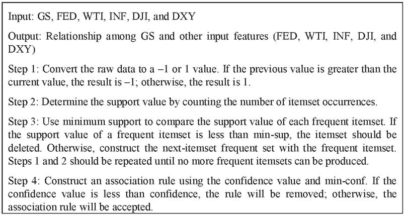
Figure 2 Association rule algorithm.
3.2.1 Determining relationships of feature using the association rule
From Figure 2, the relationships among output, GS, and all input features are determined. Then, the rules are obtained from this process. Next, the selected time-series datasets are ready for training LSTM.
3.2.2 Data preparation
Before fitting an LSTM model, some datasets must be transformed into processable LSTM input data [39]. The algorithm for data transformation is shown in Figure 3.
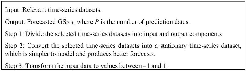
Figure 3 Data-transformation algorithm.
For this study, the time-series datasets were rescaled to values between 1 and 1, as the LSTM model expected the data to be within the network’s activation-function scale. A network structure consists of one hidden layer with one LSTM unit. Then, an output layer with a linear activation function and output values was constructed for a simple LSTM. The number of time steps over which a forecast was needed determined the value of prediction dates P. A dropout was set to 0.2. The MAPE also was represented as a loss function and a method for network optimization [40]. For both training and forecasting, the network’s batch size was set to 16.
3.3 Simulation
This process aimed to demonstrate the efficacy of the proposed gold-price forecasting method by using the simulation. The proposed forecasting method was written in Python 3 and relies on the NumPy and Pandas packages. The simulation was conducted to present a specific situation, specified by the parameters in Table 4. The comparison results are compared to those of other baseline techniques such as the simple moving average (SMA) [41], weight moving average (WMA) [42], and exponential moving average (EMA) [43], as well as auto-regressive integrated moving average (ARIMA) [40]. The simulation parameters used in the simulation are listed in Table 3.
Table 4 Simulation parameters
| Entities | Description | Detail/Range |
| Features | Features used in simulation |
1. Gold spot (GS) 2. Related inputs obtained from association rules |
| Baseline | Methods for comparison | SMA, WMA, EMA, and ARIMA |
| Past days | The number of days in the past that can be used to estimate the future | 8, 13, 55, 89, and 144 days |
| Forecasting date | The expanded forecast dates beyond the future dates that were originally set | 50 days |
| Dropout | A regularization technique that eliminates overfitting | 0.2 |
| Epoch | Training epoch | 10–500 iterations |
| Optimizer | Network optimization method | Adaptive estimates of lower-order moments [40] |
| Loss function | Measured error rate | MAPE |
| Activation | Activation function | Relu, Softmax |
4 Results and Discussion
From the process of determining features’ relationships, the derived association rules are shown in Table 5.
Table 5 Association rules for forecasting gold prices
| Rules | Support | |
| 1. | DXY - GS | 0.158 |
| 2. | GS - WTI | 0.256 |
| 3. | GS - DJI | 0.204 |
| * Control variables: Minimum support 0.15. | ||
As illustrated in Table 5, the following are the factors to consider concerning the gold price:
Rule 1: If the DXY changes, so does the gold price.
Rule 2: If the price of gold increases, so does the price of WTI.
Rule 3: If the gold price changes, so does the DJI.
As a result, Rule 1 was selected to apply to LSTM. This is because DXY affects gold prices, whereas WTI and DJI are affected by gold prices.
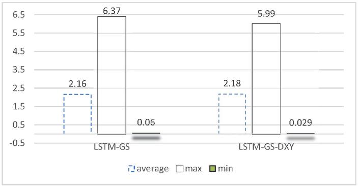
Figure 4 The MAPE error rate of the LSTM-GS in comparison to the LSTM-GS-DXY.
Figure 4 shows the performance of the LSTM model for different numbers of features: (a) one feature GS (LSTM-GS), and (b) two features: DXY with GS (LSTM-GS-DXY). The number of features is expressed on the horizontal axis, while the error rate MAPE, which calculates relative errors, is represented on the vertical axis. Figure 4 depicts the MAPE error rate’s average, maximum, and minimum values. Compared to the LSTM-GS, the proposed LSTM-GS-DXY model has a relatively equal average error rate but lower maximum and minimum error rates, respectively.
Figure 5 also provides a comparison of the actual gold prices with forecasted gold prices using (a) one feature, GS, (b) two features, GS, and DXY, and (c) one feature and two features.
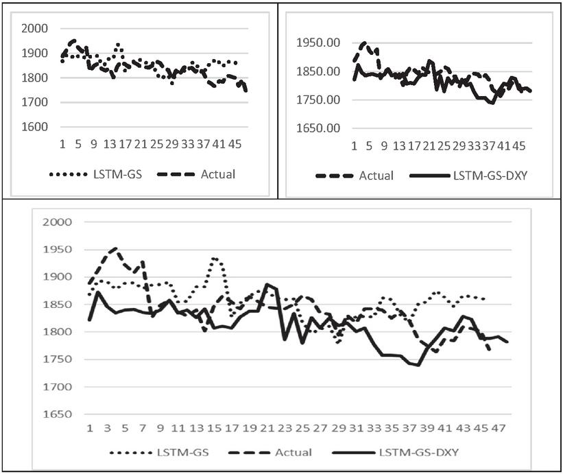
Figure 5 A comparison of actual gold prices, LSTM-GS forecasted price, and LSTM-GS-DXY forecasted price.
For LSTM training, the difference epochs obtained the difference MAPEs, as shown in Figure 6. In Figure 6, the appropriate training range is between 50 and 500 epochs for the LSTM-GS-DXY model.
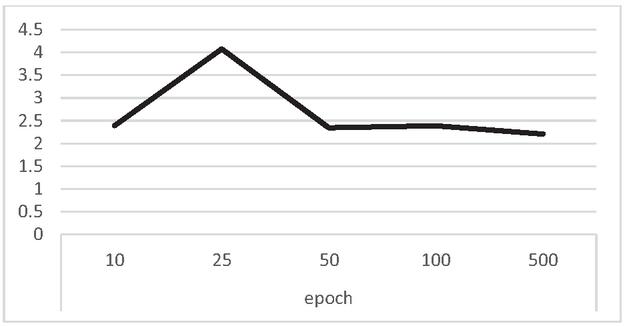
Figure 6 The error rate MAPE of the difference epochs at one feature of the LSTM-GS-DXY model.
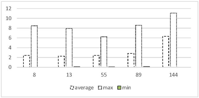
Figure 7 The LSTM-GS-DXY model’s MAPE error rate of the difference over the past days.
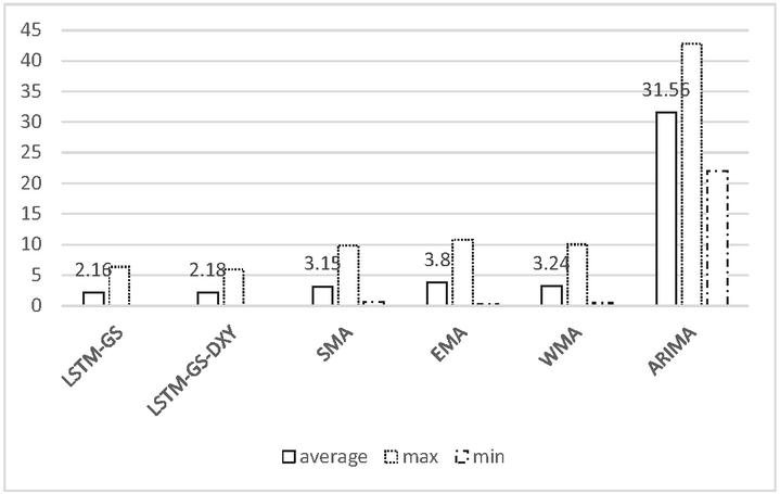
Figure 8 A comparison of the error rates of LSTM-GS, LSTM-GS-DXY, SMA, EMA, WMA, and ARIMA.
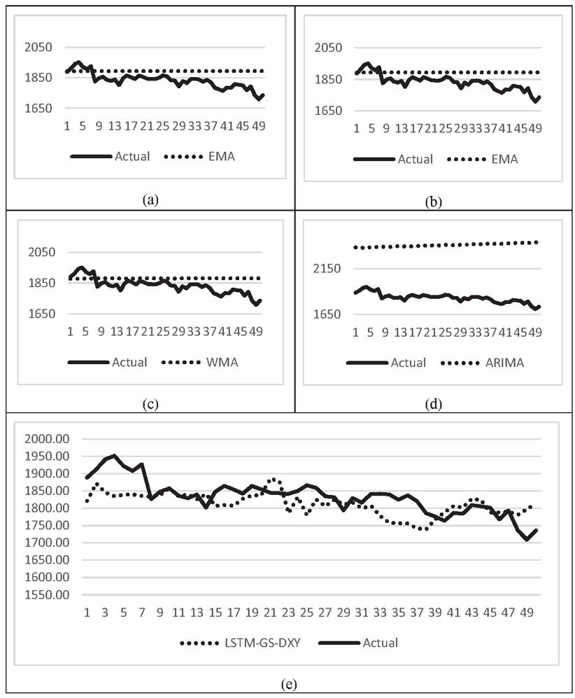
Figure 9 A comparison of actual gold prices with SMA, EMA, WMA, ARIMA, and LSTM-GS-DXY predictions.
Additionally, the performance of the LSTM-GS model on various previous days is shown in Figure 7. The number of days in the past is expressed on the horizontal axis, while the error rate MAPE is represented on the vertical axis. Figure 7 depicts that the MAPE error rate’s average, maximum, and minimum values are relatively low during the previous 8–55 days.
As previously mentioned, SMA, WMA, EMA, and ARIMA are used to compare the models to the baseline. The horizontal axis in Figure 7 represents the baseline, while the vertical axis represents the MAPE error rate. Figure 7 depicts the MAPE error rate’s average, maximum, and minimum values. Compared to all other baseline approaches, the proposed LSTM-GS-DXY system has the lowest error rates. The forecasting results indicate that the LSTM-GS-DXY is the most accurate for describing the data used in this study. Figure 8 also shows a comparison of the error rates of the actual gold price with gold-price predictions using (a) LSTM-GS, (b) LSTM-GS-DXY, (c) SMA, (d) EMA, e WMA, and (f) ARIMA over the previous 13 days.
In Figure 9, the actual gold price is compared to the gold-price forecast of the (a) SMA, (b) EMA, (c) WMA, (d) ARIMA, and (e) LSTM-GS-DXY.
As illustrated in Figures 8 and 9, when compared to the proposed LSTM-GS-DXY model to the LSTM-GS, SMA, EMA, WMA, and ARIMA, the proposed LSTM-GS-DXY has the lowest maximum and minimum error rates. Additionally, the proposed LSTM-GS-DXY has a relatively low average error rate compared to the LSTM-GS. Overall, the simulation results show that the proposed LSTM-GS-DXY outperforms other comparison methods.
5 Conclusion and Future Work
To examine with several inputs and one output in forecasting, this study proposed an LSTM system. Before processing inputs in the LSTM, this study examined the relationship between the inputs and output using association rules. This method established that the DXY influences GS. In practice, when the DXY or US Dollar Index changes, it will surpass the gold price because money will be invested in stable assets, such as gold. Using simulation software, various scenarios were created and analyzed based on features, past days, and epochs. The simulation-program results show that the LSTM-GS-DXY scheme produces the lowest MAPE. Although a difference in MAPE can be caused by a difference in past days and epochs, by using MAPE as the error metric, the proposed LSTM-GS-DXY scheme outperforms SMA, WMA, EMA, and ARIMA for forecasting gold price, thus demonstrating the utility of the proposed approach for maintaining a sustainable balance between the expected and actual gold prices. In the future, we expect to combine the proposed LSTM-GS-DXY system with other techniques to increase prediction accuracy, especially against unpredicted events such as war and pandemics that seriously affect the gold price.
Acknowledgment
The publication of this work was supported by the Gold Research Center.
References
[1] Adrangi B, Chatrath A, Raffiee K. Economic activity, inflation, and hedging: the case of gold and silver investments. The Journal of Wealth Management. 2003 Jul 31;6(2):60–77.
[2] Wang W, Xia W. Empirical Modeling for the Spot Price of Gold Based on Influencing Factors. Applied Economics and Finance. 2017;4(3):129–40.
[3] Napaaun P. The Analysis of Factors Influencing Gold Bar Price in Thailand. Thesis, Bangkok University, 2015.
[4] Board of Governors of the Federal Reserve System. (n.d.) Federal Reserve Board. Retrieved December 1, 2021, from https://www.federalreserve.gov/aboutthefed.htm.
[5] West Texas Intermediate (WTI). (n.d.) Investopedia. Retrieved March 31, 2021, from https://www.investopedia.com/terms/w/wti.asp.
[6] Who or What Is Dow Jones? (n.d.) Investopedia. Retrieved March 31, 2021, from https://www.investopedia.com/ask/answers/who-or-what-is-dow-jones/.
[7] U.S. Dollar Index (USDX). Retrieved March 31, 2021, from https://www.investopedia.com/terms/u/usdx.asp.
[8] Kroner KF, Kneafsey KP, Claessens S. Forecasting volatility in commodity markets. Journal of Forecasting. 1995 Mar;14(2):77–95.
[9] Kristjanpoller W, Minutolo MC. Gold price volatility: A forecasting approach using the Artificial Neural Network–GARCH model. Expert systems with applications. 2015 Nov 15;42(20):7245–51.
[10] Tealab, A., 2018. Time series forecasting using artificial neural networks methodologies: A systematic review. Future Computing and Informatics Journal, 3(2), pp. 334–340.
[11] Tully E, Lucey BM. A power GARCH examination of the gold market. Research in International Business and Finance. 2007 Jun 1;21(2):316–25.
[12] Trück S, Liang K. Modelling and forecasting volatility in the gold market. International Journal of Banking and Finance. 2012 Mar 22;9(1):48–80.
[13] Xu Q, Deng K, Jiang C, Sun F, Huang X. Composite quantile regression neural network with applications. Expert Systems with Applications. 2017 Jun 15;76:129–39.
[14] Hafezi R, Akhavan A. Forecasting gold price changes: Application of an equipped artificial neural network. AUT Journal of Modeling and Simulation. 2018 Jun 1;50(1):71–82.
[15] Schmidhuber J. Deep learning in neural networks: An overview. Neural networks. 2015 Jan 1;61:85–117.
[16] Zhou S, Lai KK, Yen J. A dynamic meta-learning rate-based model for gold market forecasting. Expert Systems with Applications. 2012 May 1;39(6):6168–73.
[17] Zhang P, Ci B. Deep belief network for gold price forecasting. Resources Policy. 2020 Dec 1;69:101806.
[18] Fischer T, Krauss C. Deep learning with long short-term memory networks for financial market predictions. European Journal of Operational Research. 2018 Oct 16;270(2):654–69.
[19] Livieris IE, Pintelas E, Pintelas P. A CNN–LSTM model for gold price time-series forecasting. Neural computing and applications. 2020 Dec;32(23):17351–60.
[20] Khani MM, Vahidnia S, Abbasi A. A Deep Learning-Based Method for Forecasting Gold Price with Respect to Pandemics. SN Computer Science. 2021 Jul;2(4):1–2.
[21] Agrawal R, Imieliñski T, Swami A. Mining association rules between sets of items in large databases. In Proceedings of the 1993 ACM SIGMOD international conference on Management of data 1993 Jun 1 (pp. 207–216).
[22] Karabatak M, Ince MC. A new feature selection method based on association rules for diagnosis of erythemato-squamous diseases. Expert Systems with Applications. 2009 Dec 1;36(10):12500–5.
[23] Huang C, Huang X, Fang Y, Xu J, Qu Y, Zhai P, Fan L, Yin H, Xu Y, Li J. Sample imbalance disease classification model based on association rule feature selection. Pattern Recognition Letters. 2020 May 1;133:280–6.
[24] Qu Y, Fang Y, Yan F. Feature selection algorithm based on association rules. In Journal of Physics: Conference Series 2019 Feb 1 (Vol. 1168, No. 5, p. 052012). IOP Publishing.
[25] Kaur M, Kang S. Market Basket Analysis: Identify the changing trends of market data using association rule mining. Procedia computer science. 2016 Jan 1;85:78–85.
[26] Gupta S, Mamtora R. A survey on association rule mining in market basket analysis. International Journal of Information and Computation Technology. 2014;4(4):409–14.
[27] Sagin AN, Ayvaz B. Determination of association rules with market basket analysis: application in the retail sector. Southeast Europe Journal of Soft Computing. 2018 May 10;7(1).
[28] Na SH, Sohn SY. Forecasting changes in Korea composite stock price index (KOSPI) using association rules. Expert Systems with Applications. 2011 Jul 1;38(7):9046–9.
[29] Cheng CH, Chen CH. Fuzzy time series model based on weighted association rule for financial market forecasting. Expert Systems. 2018 Aug;35(4):e12271.
[30] Lee SI, Yoo SJ. Multimodal deep learning for finance: integrating and forecasting international stock markets. The Journal of Supercomputing. 2020 Oct;76(10):8294–312.
[31] Xia X. Learning behavior mining and decision recommendation based on association rules in interactive learning environment. Interactive Learning Environments. 2020 Aug 4:1–6.
[32] Dahdouh K, Dakkak A, Oughdir L, Ibriz A. Association rules mining method of big data for e-learning recommendation engine. InInternational Conference on Advanced Intelligent Systems for Sustainable Development 2018 Jul 12 (pp. 477–491). Springer, Cham.
[33] Intayoad W, Becker T, Temdee P. Social context-aware recommendation for personalized online learning. Wireless Personal Communications. 2017 Nov;97(1):163–79.
[34] Smagulova K, James AP. Overview of long short-term memory neural networks. InDeep Learning Classifiers with Memristive Networks 2020 (pp. 139–153). Springer, Cham.
[35] Hochreiter S, Schmidhuber J. Long short-term memory. Neural computation. 1997 Nov 15;9(8):1735–80.
[36] Sivalingam KC, Mahendran S, Natarajan S. Forecasting gold prices based on extreme learning machine. International Journal of Computers Communications & Control. 2016 Mar 24;11(3):372–80.
[37] He Z, Zhou J, Dai HN, Wang H. Gold price forecast based on LSTM-CNN model. In2019 IEEE Intl Conf on Dependable, Autonomic and Secure Computing, Intl Conf on Pervasive Intelligence and Computing, Intl Conf on Cloud and Big Data Computing, Intl Conf on Cyber Science and Technology Congress (DASC/PiCom/CBDCom/CyberSciTech) 2019 Aug 5 (pp. 1046–1053). IEEE.
[38] Livieris IE, Pintelas E, Pintelas P. A CNN–LSTM model for gold price time-series forecasting. Neural computing and applications. 2020 Dec;32(23):17351–60.
[39] Lewis ND. Deep Time Series Forecasting with Python. Create Space Independent Publishing Platform. 2016 Dec.
[40] Kingma DP, Ba J. Adam: A method for stochastic optimization. arXiv preprint arXiv:1412.6980. 2014 Dec 22.
[41] Hansun S. A new approach of moving average method in time series analysis. In2013 conference on new media studies (CoNMedia) 2013 Nov 27 (pp. 1–4). IEEE.
[42] Zhang Z, Qiao Y, Zhang T, Lu Y. Fractional weight moving average based thresholding scheme for VLC with mobile-phone camera. IEEE Photonics Journal. 2019 Jan 21;11(1):1–8.
[43] Klinker F. Exponential moving average versus moving exponential average. Mathematische Semesterberichte. 2011 Apr;58(1):97–107.
Biographies

Laor Boongasame is currently a Lecturer with the School of Science, King Mongkut’s Institute of Technology Ladkrabang, Bangkok, Thailand. She received the Ph.D. degree in computer engineering from the King Mongkut’s University of Technology Thonburi, Thailand. Her research interests involve buyer coalitions, n-person game theory, and investment. She has published several research papers in internationally refereed journals and has presented several papers at several international conferences.

Piboonlit Viriyaphol is currently a Director of Gold Research Center, a research and development unit at Gold Traders Association, Bangkok, Thailand. He received the B.Eng. degree in computer engineering in 1996 from Kasetsart University, Thailand. He received the M.Sc. degree in computer information system, in 2000, and the Ph.D. degree in telecommunication science, in 2006, from Assumption University, Thailand. He has been working with many universities in Thailand, such as Bangkok University, Assumption University, and King Mongkut’s Institute of Technology Ladkrabang, Bangkok Thailand, for both communication-based and financial-market-related research. His areas of research interests include traffic engineering, routing techniques, approximation techniques, and price modeling and forecasting in commodity market.

Kriangkrai Tassanavipas is currently the Director of Innovation and Invention Excellence Center (IIEC), Faculty of Engineering and Technology, Panyapiwat Institute of Management, Bangkok, Thailand. He received the B.Eng. degree in computer engineering, the M.Eng. degree in electrical engineering, respectively, from the Prince of Songkla University, and the Ph.D. degree in robotics and automation from the King Mongkut’s University of Technology Thonburi, Thailand. His research interests include robotic and automation, computer vision, IoT (Internet of Things), artificial intelligence, and biomedical engineering fields. He has experience working with large companies in Thailand such as CPALL, FORD, ABB, etc. Also, he has been a guest speaker for Thailand’s universities including King Mongkut’s Institute of Technology Ladkrabang, Prince of Songkla University, Maidol University, etc.

Punnarumol Temdee received the B.Eng. degree in electronic and telecommunication engineering, the M.Eng. degree in electrical engineering, and the Ph.D. degree in electrical and computer engineering from the King Mongkut’s University of Technology Thonburi. She is currently a Lecturer with the School of Information Technology, Mae Fah Luang University, Thailand. Her research expertise is in artificial intelligence-based application, context-aware computing, and pattern classification.
Journal of Mobile Multimedia, Vol. 19_1, 165–186.
doi: 10.13052/jmm1550-4646.1919
© 2022 River Publishers