Empirical Model for Total Precipitable Water Retrieval from Ground-based GNSS Observations in Thailand

Yuttapong Rangsanseri^1,*, Weeranat Phasamak¹, and Seubson Soisuvarn²

¹Faculty of Engineering, King Mongkut’s Institute of Technology Ladkrabang, Ladkrabang, Bangkok, Thailand

²NOAA/NESDIS/Center for Satellite Applications and Research, College Park, MD, USA

E-mail: yuttapong.ra@kmitl.ac.th; 59601303@kmitl.ac.th; seubson.soisuvarn@noaa.gov

* Corresponding Author

Received 23 January 2019; Accepted 02 June 2020; Publication 17 August 2020

Abstract

Retrieval of Total Precipitable Water (TPW) from ground-based Global Navigation Satellite System (GNSS) observations is a challenging task due to its real-time and high temporal resolution nature. In this paper, we present a method for establishing an analytical model for retrieving the TPW based on the GNSS observations over 1-year period from 12 stations distributed across Thailand. The derived Zenith Total Delay (ZTD) at all stations agrees well with the TPW data available from the Global Data Assimilation System (GDAS) Numerical Weather Prediction (NWP) model. First, a unique relationship between the ZTD and the TPW was established by taking into account the variations in station altitudes. Then, a bias correction technique with Probability Distribution Function (PDF) matching was applied to improve the final model. The inversion model of the TPW from ZTD was then easily obtained by using a numerical technique. The performance of our method has been successfully evaluated on an independent test data. This model can be useful for near real-time TPW measurements from globally available GNSS receivers.

Keywords: GNSS Remote Sensing, Zenith Total Delay, Total Precipitable Water, PDF Matching.

1 Introduction

Total precipitable water (TPW) is the total amount of water in the Earth’s atmosphere derived by integrating all the water vapor in columns of atmosphere from the surface to the top of the atmosphere, measured in kilograms per square meter (kg/m²) or equivalently in millimeter (mm) of condensate units. Further, TPW is one of many geophysical variables that can help us better understand our complex Earth systems that play essential roles in climate change. There are several methods to derive atmospheric TPW, for example, direct measurements using the vertical profile of atmospheric temperature, humidity and other related atmospheric parameters, and indirect measurements from passive satellite microwave radiometers [1].

Measurement of the TPW field from microwave radiometers can be used to determine the precipitation potential in an operational weather forecast. Observations from an Advanced Microwave Scanning Radiometer—Earth Observing System (AMSR-E) [2] and a Tropical Rainfall Measuring Mission (TRMM) Microwave Imager (TMI) [3] have been assimilated in a Meso-scale Analysis by the Japan Meteorological Agency (JMA) [4].

Zenith total delay (ZTD) measures the delay of a signal received from a Global Navigation Satellite System (GNSS) satellite at zenith direction, caused by the presence of neutral atmosphere and expressed as excess path length. The ZTD has two components: a delay due to hydrostatic pressure and one due to the amount of water vapor along the ray path. The ZTD depends on the surface pressure and the TPW content above the GNSS receiving station [5]. Signals broadcast by the Global Positioning System (GPS) satellites have been used since 1992 to monitor the atmosphere from ground-based stations. This type of sensor was first used by Bevis et al [6]. Generally, slow variation in the ZTD is due to hydrostatic component, whereas more rapid change is due to variation in water vapor [7]. The ZTD observations in numerical weather prediction (NWP) models have previously been studied [8–10]. Faccani et al. investigated the impact of the ZTD data collected by 15 GPS stations at a LAM center in the Basilicata region in Italy for the winter of 2003 and spring of 2004. They used the 3-Dimensional VARiational (3DVAR) assimilation scheme. They improved mean and Root Mean Square (RMS) errors in rainfall forecasts, using the ZTD data compared to rain gauges [11].

The TPW data have been derived from the ZTD data collected by a vast network of ground-based GPS stations covering the continental United States. The TPW retrievals were assimilated in a rapid update cycle. With this approach, Gutman et al. [12] demonstrated a clear positive impact when they assimilated the GPS TPW into the 3-hour predictions of humidity. Holben et al. [13] estimated the TPW using the Japanese Geostationary Meteorology Satellite (GMS) over a tropical ocean surface and concluded that the GMS data were appropriate in mapping water vapor content. It is clear that estimation of water vapor over oceans is easy, because emissivity and temperature of the ocean surface are relatively constant [14]. For effective use of atmospheric moisture information, sensed from the ground-based GNSS stations, data processing and delivery must be timely, preferably available in less than one hour [15]. An approximately 15-minute latency of the TPW data input into the NWP models was the target for the GNSS Meteorological products. The TPW has been derived from the ZTD using Wang et al.’s physical-based technique [16].

We developed an empirical relationship between the ground based GNSS ZTD observations and TPW data, available from an NWP model. We collected the ZTD data from existing the GNSS receiving stations in Thailand and the TPW data from the NWP model of the Global Data Assimilation System (GDAS). Collocation from these two data sources is described in Section 2. A preliminary relationship between the ZTD and TPW is presented in Section 3, followed by a refined and final model in Section 4. Section 5 presents the implementation of the final model, derived in Section 4, in which the TPWs were retrieved and validated. We present our conclusions in Section 6.

2 Collocating ZTD with TPW

We used two datasets to train our empirical model. The first was the GNSS ZTD data from July 2017 to August 2018. The ZTD data was obtained from GNSS receivers controlled by the Thai GNSS and Space Weather Information Data Center at King Mongkut’s Institute of Technology Ladkrabang (KMITL), Thailand [17], and from the Department of Public Works and Town and Country Planning, Ministry of Interior, Thailand. We used 12 GPS receivers from different locations across Thailand, namely, NKNY, SPBR, PJRK, CHAN, CPN, SOKA, NKSW, KMT1, KMT2, DPT9, NKNI, and CMU. The locations and their altitudes are shown in Figure 1.

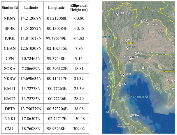
Figure 1 Positions and altitudes of GPS receiver stations used (left) and a map of Thailand (right).

2.1 ZTD Data

To train the model, raw GPS data needed to be processed first. We used RTKLIB (RTKPOST, postprocessing analysis) software to produce a file that contained the ZTD data in millimeters. Data from the KMITL GNSS base stations and the Department of Public Works and Town & Country Planning stations were in a Receiver Independent Exchange (RINEX) format. A RINEX Navigation message file, with precise satellite ephemeris and satellite clock was used to compute the ZTD. The RTKPOST settings are shown in Table 1. The estimated ZTD output was at 60-second intervals. Each hourly interval was then averaged to produce one hour resolution data.

Bad data from the ZTD signal collection were excluded. The NNKI station was the source of most missing and noisy data. A time series of the ZTD signals over a 1-year period (July 2017 and August 2018) showed similar characteristics (Figure 2). In the winter months, the amount of water vapor in the atmosphere was low, resulting in lower ZTD values (Figure 2). In the next step, we used these ZTD signals to collocate with the TPW data from each station.

Table 1 RTKPOST Settings

Positioning Mode	PPP Fixed
Frequency/Filter Type	L1+L2, Combined
Elevation Mask (°)	15
Earth Tide Correction	Solid
Ionosphere Correction	Estimate TEC
Troposphere Correction	Estimate ZTD
Satellite Ephemeris/Clock	Precise
Datum/Height	WGS84/Ellipsoidal
Rover	X/Y/Z-ECEF(m)

2.2 TPW Data

The TPW is one of many meteorological parameters in gridded output fields in an NWP model, which are used to collocate with ZTD. Here, the TPW was obtained from the GDAS NWP model. The GDAS that we used had a resolution of 0.25° in both latitude and longitude. The GDAS model output data was produced four times a day, at 00, 06, 12, and 18 UTC. To map the TWP to the GNSS receiver locations, we needed to interpolate the TPW to the exact location and time of each station. Since the TPW value from the GDAS was gridded at approximately 25 km × 25 km, to find a TPW value at the location of the GNSS station location, we temporally interpolated the TPW values between the GDAS cycles to match the ZTD values. The relationship between the interpolated TPW value and the ZTD value at each station was then determined, as discussed in the next section.

2.3 ZTD and TPW Relationship

After the ZTD and TPW values were obtained for all the 12 GNSS receiver stations, we established an empirical relationship between the ZTD and TPW. The time series of the ZTD and TPW for every station is shown in Figure 2. Since these ZTD data were still very noisy, we averaged them over 3,600-second intervals to reduce noise. Figure 2 shows that the ZTD observations correlated very well with the TPW values calculated for all stations, except the NNKI station, where there was a large number of missing data, where poor quality data had been rejected by quality control. Over a 1-year period (July 2017–August 2018), a seasonal fluctuation of the ZTD, caused by the TPW, especially a decrease in the TPW, during the winter months (˜December–February), can be seen clearly. The seasonal ZTD fluctuation was due to the fluctuation in relative humidity.

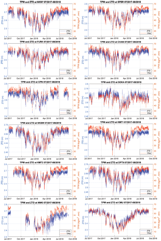
Figure 2 TPW collocated with ZTD observed at 12 GNSS stations in Thailand.

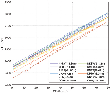
Figure 3 Relationships between TPW and ZTD for each station.

We then bin-averaged the TPW at 2-mm bins, so that they correlated well with the ZTD. The ZTD, as a function of the TPW, was then plotted (Figure 3 [dash line]), with the graph showing an almost linear relationship. However, there appeared to be a different offset for each station. This was largely caused by the difference in signal delay to stations, located at different altitudes. The linear regression equations for the ZTD vs TPW for each station are presented in (1) and shown as solid lines in Figure 3:

$$\begin{array}{r}\begin{array}{rl}ZT{D}_{NNKY}& =5.7699\ast TP{W}_{NNKY}+2344.5981\\ ZT{D}_{SPBR}& =5.4733\ast TP{W}_{SPBR}+2347.5062\\ ZT{D}_{PJRK}& =5.5909\ast TP{W}_{PJRK}+2364.9656\\ ZT{D}_{CHAN}& =5.7592\ast TP{W}_{CHAN}+2351.0948\\ ZT{D}_{CPN}& =5.8509\ast TP{W}_{CPN}+2331.1833\\ ZT{D}_{SOKA}& =5.8077\ast TP{W}_{SOKA}+2349.7293\\ ZT{D}_{NKSW}& =5.2141\ast TP{W}_{NKSW}+2356.6251\\ ZT{D}_{KMT1}& =5.5506\ast TP{W}_{KMT1}+2322.0873\\ ZT{D}_{KMT2}& =5.5841\ast TP{W}_{KMT2}+2327.3091\\ ZT{D}_{DPT9}& =5.3745\ast TP{W}_{DPT9}+2342.7058\\ ZT{D}_{NNKI}& =5.4509\ast TP{W}_{NNKI}+2300.7617\\ ZT{D}_{CMU}& =6.0648\ast TP{W}_{CMU}+2252.4613\end{array}\end{array}$$

(1)

where ZTD_s was the ZTD at station s and TPW_s was the collocated TPW at the same station. The slope of the ZTD (mm) per TPW (mm) for every station was close to the mean slope of $\tilde{5}\text{.}6$ mm/mm. However, the offsets differed between stations, because of altitude differences, that we will address in Section 3.

3 Modeling of ZTD

We have seen that the ZTD depended on both the TPW and GNSS receiver station altitudes. To simplify the problem, we derived a relationship between the ZTD and the TPW for all stations in a generic form, by first considering only the effect of altitude and then finding the effect of the TPW. Finally, we combined the two effects together into a final form.

3.1 Ellipsoidal Height Dependency

Based on 1-year GNSS data and Thailand’s geophysical area, the most frequently occurring of TPW was in the range of 50–52 mm. We then decided to use the TPW value at this bin to find the relationship between the ZTD and altitude. The mean ZTDs associated with the TPW in the 50–52 mm bin for every station were plotted against station altitude in Figure 4: this showed that the ZTD decreased logarithmically with altitude, i.e., fitted a model in the form of a∗log(b∗h + 1) + c. The coefficients in this model that best fitted the data are shown in (2):

$$W\left(h\right)=-48.64\ast log(0.0128\ast h+1)+2640,$$

(2)

where W is the ZTD in the TPW 50–52 bin and h represents the ellipsoidal height in meters. This equation is valid for h ≥ −1/0.0128, about −78 m.

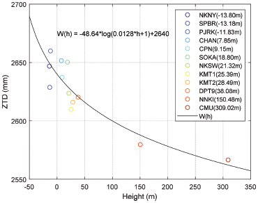
Figure 4 Relationship between the ZTD and ellipsoidal height for TPW bin at 50–52 mm.

3.2 TPW Dependency

We removed the ZTD altitude dependency for each station at their respective altitudes by subtracting (2) from (1). This aligned the ZTDs for all the 12 stations. The results are shown in Figure 5. The ZTDs for all the 12 stations were then close to linearly dependent on the TPW.

A linear regression analysis showed that the relationship between the ZTD and TPW can be modeled as:

$$ZT{D}_0=5.682\ast TPW-294.7,$$

(3)

where ZTD₀ is the ZTD with no height dependency.

3.3 Combining the Model

As mentioned earlier, the ZTD was dependent on both the TPW and ellipsoidal station height. By combining (2) and (3) we obtained a preliminary model for the ZTD at any station as

$$M(tpw,h)=5.682\ast tpw-48.64\ast log(0.0128\ast h+1)+2345.3$$

(4)

where M is the preliminary model of the ZTD given the tpw and h. This shows that the ZTD signals decreased logarithmically with height and linearly increased with TPW with a slope of 5.682 mm/mm. This means that for every 1 mm change in the TPW, there was a change of 5.682 mm in the ZTD delay signal.

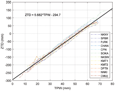
Figure 5 ZTD vs TPW after removal of altitude dependency.

To validate the accuracy of this model, we plotted M(tpw,h) as a function of the TPW for every station by substituting h for the actual altitude in (4). The resulting 12 solid curves for each site (in Figure 3) were overlaid with obtained measurement data (dash line). The results are shown in Figure 6. It is clear that the preliminary ZTD model obtained in (4) was consistent with the observation data.

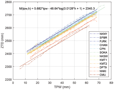
Figure 6 Preliminary model with observation data from 12 stations.

Table 2 Differences between calculated and observed ZTDs

		Ellipsoidal	Error (mm)
No.	Station Id.	Height (m)	Mean	S.D.
1	NKNY	-13.80	-2.94	18.80
2	SPBR	-13.18	-15.79	19.90
3	PJRK	-11.83	13.54	18.38
4	CHAN	7.86	19.62	18.49
5	CPN	9.15	6.31	18.74
6	SOKA	18.81	23.91	17.41
7	NKSW	21.32	0.29	20.29
8	KMT1	25.39	-13.70	17.55
9	KMT2	28.49	-5.12	18.11
10	DPT9	38.08	2.60	16.85
11	NNKI	150.48	-1.02	30.75
12	CMU	309.02	2.13	20.60

The differences between the ZTD calculated from the model and the observed ZTD data at each station were reported as mean errors and standard deviation (Table 2). The overall bias and standard deviation calculated from all the 12 stations data were 2.42 mm and 22.81 mm.

4 Fine-Tuning the Model

4.1 ZTD Residual Errors

In Figure 7, the mean difference (bias) between the measured data and data calculated from the ZTD model is shown as a function of the TPW. The error bars indicate the standard deviation of the difference at each TPW bin. We did not consider differences for TPW < 10 mm and TPW > 70 mm to be statistically significant, because of small number of the data points. Therefore, we decided to quality control the mean difference within the TPW range between 10 and 70 mm as shown in Figure 7. The mean bias for the TPW between 60 and 70 mm had a negative slope, indicating that the model was overestimated linearly over the ZTD. We believe that the residual errors in this TPW range were either because the simple linear model was not able to capture the GNSS ZTD signal accurately or because the GNSS ZTD had become saturated beyond TPW > 60 mm. The situation for TPW > 60 mm is beyond the scope of this paper; therefore, here, we focused only on correcting the residual errors of the ZTD model for the 10–60 mm range of the TPW. Nevertheless, we believe that the model is practically valid for the entire range of possible TPW even though some residual error may still remain.

4.2 Bias Correction with PDF Matching

One way to correct the residual error in the ZTD model is by using a Probability Distribution Function (PDF) matching technique described hereunder. This technique aims to compute a correction to a variable, in this case a ZTD model, so that the resulting corrected values “matched” underlining reference values. In our case, we computed the ZTD correction (ΔZTD) to the preliminary ZTD model so that the corrected ZTD model “matched” the observed ZTD. Instead of “matching” the PDF directly, we derived the correction through a Cumulative Distribution Function (CDF), since the PDF is the derivative of the CDF and the CDF correction is more easily implemented. Figure 8(a) shows the CDF of the observed ZTD and the preliminary ZTD model. The ZTD correction (ΔZTD) to the preliminary ZTD model that results in a “match” between the PDF of the corrected model and the PDF of the observed ZTD is shown as the red curve in Figure 8(b). In order to cover the full ZTD range, we implemented a third-order polynomial fit to the data

$$\mathrm{\Delta }ZTD\left(x\right)=-3.409\ast x^3+{1.788}^{\ast }{x}^2-4.634\ast x+1.842$$

(5)

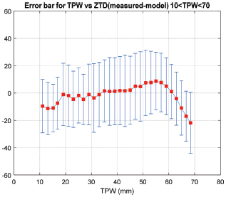
Figure 7 Mean differences between the observed and calculated ZTD as a function of TPW. Error bars were derived from measured and model.

where x is the preliminary model and M (tpw,h) was calculated by (4). Finally, we combined (4) and (5) to form the final ZTD model:

$$ZTD(tpw,h)=5.682\ast tpw-48.64\ast log(0.0128\ast h+1)+2345.3-\mathrm{\Delta }ZTD$$

(6)

To verify the validity of the residual error correction, we drew density scatter plots between the measured ZTD and the model (Figure 9), showing the residual error before and after correction. The average error of the means for the final model decreased from 2.42 to −0.37 with a comparable standard deviation with respect to the preliminary model. However, the final residual error for TPW > 60 mm remained underestimated relative to the observed signal as described in Section 4.1.

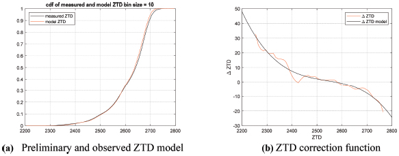
Figure 8 (a) CDF of the preliminary ZTD model and the observed ZTD. (b) ZTD correction function for the preliminary ZTD model.

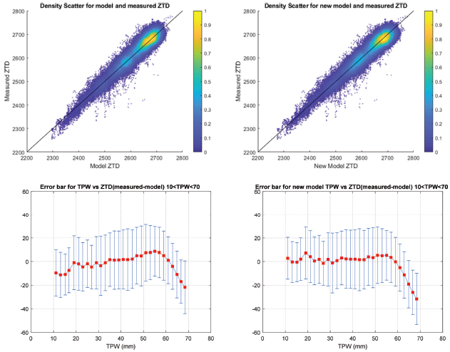
Figure 9 Density scatter plots and mean error bars of the preliminary model (left) and the final model (right).

5 TPW Retrieval

5.1 TPW Inversion Method

We can solve for the TPW using the ZTD model derived in (6). We used maximum likelihood estimation to search for the TPW solutions. Given a GNSS receiver station altitude, we searched through all possible TPW values within a [0, 80] mm range in 0.1 mm step resolution and found the TPW that minimized the cost function:

$$\mathrm{Cost\; function}=\frac{{(ZTD-M(tpw,h))}^2}{std},$$

(7)

where std is the standard deviation of the M(tpw,h). The value for the std was 23.18 mm (Figure 10b) which was the standard deviation of the entire observation data from all the GNSS receiver stations in the period between July 2017 and August 2018.

The resulting TPW retrieval values for the whole observation period are shown in Figure 10. Figure 10a shows the histogram of the differences between retrieved TPW and TPW trained by the GDAS, with a mean bias of 0.059 mm and a standard deviation of 3.83 mm. Figure 10c compares the TPW PDFs from the retrieval and the GDAS. Figure 10d shows the TPW scatter plots.

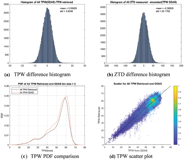
Figure 10 TPW retrieval from ZTD model. (a) TPW difference histogram. (b) ZTD difference histogram. (c) TPW PDF comparison and (d) TPW scatter plots.

5.2 Validation Result

To validate our TPW retrieval results, we selected an independent ZTD dataset from the KMT2 station over a 1-month period in January 2019 and ran the model on it. The resulting TPW time series is shown as the blue curve in Figure 11a, and the corresponding TPW from the GDAS is shown as the red curve. Although there was some noise in the retrieval, one can see that the retrieved TPW tracked that of the GDAS TPW very well. This noise could be easily reduced by using a sample average running window. Figure 11b shows the histogram of the TPW difference. The mean bias was 1.8337, and the standard deviation was 2.8. The TPW accuracy of 2.8 was comparable to the radiometer retrieval and the GPS retrieval from Mears et al. [1]. The statistics would be significantly improved with a sample average running window.

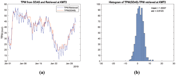
Figure 11 TPW retrieval from KMT2 station.

6 Conclusion

The Zeneith Total Delay (ZTD) is a measurement of the delay in receiving signals from Global Navigation Satellite System (GNSS) satellites which are caused mainly by the presence of the atmospheric water along its path to the surface. The ZTD delay signal provided us with an opportunity to measure the TPW indirectly. We processed the ZTD signals from the 12 GNSS ground base stations located at different altitudes in Thailand and then collocated the ZTD with the TPW variables in the GDAS NWP model to develop a forward model empirically. We found that the ZTD signals decreased logarithmically with height and linearly increased with the TPW with a sensitivity of 5.682 mm/mm. The residual errors were further corrected by using a PDF matching technique. The final model exhibited a standard deviation of 23 mm. The resulting model was tested for the TPW retrieval using an independent dataset from a single GNSS station over a month of data: the TPW retrieval showed a standard deviation of 2.8 mm. This model is very straightforward to implement and can produce the TPW measurements within an acceptable accuracy from the ZTD observations; making it suitable to be used in the existing ground-based GNSS receivers to generate the TPW measurements in near real-time.

Acknowledgments

We would like to thank Professor Pornchai Supnithi of the KMITL for his kind advice and useful suggestions about this research topic and the Department of Public Works and Town & Country Planning for providing us with the GNSS data.

References

[1] Mears, C. A., J. Wang, D. Smith, F. J. Wentz, “Intercomparison of Total Precipitable Water Measurements Made by Satellite-Borne Microwave Radiometers and Ground-Based GPS Instruments,” Journal of Geophysical Research: Atmospheres, 120, pp. 2492–2504, 2015.

[2] T. Kawanishi, T. Sezai, Y. Ito, K. Imaoka, T. Ishido, A. Shibata, M. Inahata, R. W. Spencer, “The Advanced Microwave Scanning Radiometer for the Earth Observing System (AMSR-E),” Geosci. Remote Sens., 41, pp. 184–194, 2003.

[3] Wentz, F. J., “A 17-Year Climate Record of Environmental Parameters Derived from the Tropical Rainfall Measuring Mission (TRMM) Microwave Imager,” Journal of Climate, 28, pp. 6882–6902, 2015.

[4] Japan Meteorological Agency, “Outline of Operational Numerical Weather Prediction at Japan Meteorological Agency,” http://www.jma. go.jp/jma/jma-eng/jma-center/nwp/outline-nwp/index.htm.

[5] L. Bengtsson, “The Use of GPS Measurements for Water Vapour Determination,” Bull. Amer. Meteor. Soc., 84, pp. 1249–1258, 2003.

[6] M. Bevis, S. Businger, T. Herring, C. Rocken, R. Anthes, R. Ware, “GPS Meteorology: Remote Sensing of Atmospheric Water Vapor using the Global Positioning System,” J. Geophys. Res., 97, pp. 787–801, 1992.

[7] P. Poli, P. Moll, F.-Z. EL Guelai, S.B. Healy, E. Andersson, “Forecast Impact Studies of Zenith Total Delay Data from European Near Realtime GPS Stations in Météo France 4DVAR,” J. Geophys. Res., 112, 2007.

[8] K. Boniface, V. Ducrocq, G. Jaubert, X. Yan, P. Brousseau, F. Masson, C. Champollion, J. Chery, E. Doerflinger, “Impact of High-resolution Data Assimilation of GPS Zenith Delay on Mediterranean Heavy Rainfall Forecasting,” Ann. Geophys., 27, pp. 2739–2753, 2009.

[9] S. R. Macpherson, G. Deblonde, J. M. Aparicio, B. Casati, “Impact of NOAA Ground-based GPS Observations on the Canadian Regional Analysis and Forecast System,” Mon. Wea. Rev., 136, pp. 2727–2746, 2008.

[10] H. Vedel, and X.-Y. Huang, “Impact of Ground based GPS Data on Numerical Weather Prediction,” J. Meteor. Soc., 82, pp. 459–472, 2004.

[11] C. Faccani, R. Ferretia, R. Pacione, T. Paolucci, F. Vespe, L. Cucurull, “Impact of a High Density GPS Network on the Operational Forecast,” Adv. Geosci., 2, pp. 73–76, 2005.

[12] Gutman, S. I., S. R. Sahm, S. G. Benjamin, B. E. Schwartz, K. L. Holub, J. Q. Stewart, T. L. Smith, “Rapid Retrieval and Assimilation of Ground-based GPS Precipitable Water Observations at the NOAA Forecast Systems Laboratory: Impact on Weather Forecasts,” J. Meteorol. Soc. Jpn., 82, pp. 351– 360, 2004.

[13] T.Aoki, T.Inoue, “Estimation of the Precipitable Water from the IR Channel of the Geostationary Satellite,” Remote Sensing of Environment, 12, 219–228, 1982.

[14] B. N. Holben, T. Eck, “Precipitable Water in Sahel Measured using Sunphotometry,” Agric. and Forest Meteo, 52, 95–107, 1990.

[15] J. Jones, “An Assessment of The Quality of GPS Water Vapour Estimates and Their Use in Operational Meteorology and Climate Monitoring,” PhD thesis, Institute of Engineering Surveying and Space Geodesy, University of Nottingham. 2010.

[16] J. Wang, L. Zhang, A. Dai, T. Van Hove, J. Van Baelen, “A Near-global, 2-hourly Data Set of Atmospheric Precipitable Water from Ground-based GPS Measurements,” J. Geophys. Res., 112, D11107.

[17] Thai GNSS and Space Weather Information Data Center, http://iono-gnss.kmitl.ac.th

Biographies

Yuttapong Rangsanseri received his B.Eng. and M.Eng. degrees in electrical engineering from the King Mongkut’s Institute of Technology Ladkrabang (KMITL), Thailand, in 1985 and 1987, respectively, and his Ph.D. degree from the Institute National Polytechnique de Grenoble, France, in 1992. He is currently an associate professor in the Department of Telecommunications Engineering at the KMITL. His research interests include image processing, pattern reognition, and remote sensing.

Weeranat Phasamak received his B.Eng. degree in telecommunication engineering and M.Eng. degree in electrical engineering, both from the King Mongkut’s Institute of Technology Ladkrabang (KMITL). He is currently pursuing his doctoral degree in electrical engineering at the KMITL. His research interests include Global Navigation Satellite System (GNSS) remote sensing, signal and image processing, and communication systems.

Seubson Soisuvarn received his B.Eng. degree in electrical engineering from the Kasetsart University, Bangkok, Thailand, in 1998, and the M.S.E.E. and Ph.D. degrees in electrical engineering from the University of Central Florida, Orlando, FL in 2001 and 2006, respectively.

Since 2006, he has been with the Ocean Surface Winds Team as a UCAR Project Scientist at the Center for Satellite Applications and Research, National Environmental Satellite, Data, and Information Service (NESDIS), National Oceanic and Atmospheric Administration (NOAA). His research interests include active and passive microwave remote sensing, scatterometer wind retrieval algorithm and product development, and GNSS reflectometry of ocean surface winds and waves. He has worked on calibration and validation of scatterometers from ASCAT, Oceansat-2, RapidScat, ScatSAT-1,GNSS reflectometry from TechDemoSat-1, and CYGNSS. He has developed a high wind geophysical model function (CMOD5.H) for C-band scatterometer that has been operationally utilized by the US National Weather Service. He is currently working on operational wind data products from the ScatSAT-1 to be utilized by NOAA.

Journal of Mobile Multimedia, Vol. 16_1-2, 161–180.
doi: 10.13052/jmm1550-4646.16128
© 2020 River Publishers

Abstract

1 Introduction

2 Collocating ZTD with TPW

2.1 ZTD Data

2.2 TPW Data

2.3 ZTD and TPW Relationship

3 Modeling of ZTD

3.1 Ellipsoidal Height Dependency

3.2 TPW Dependency

3.3 Combining the Model

4 Fine-Tuning the Model

4.1 ZTD Residual Errors

4.2 Bias Correction with PDF Matching

5 TPW Retrieval

5.1 TPW Inversion Method

5.2 Validation Result

6 Conclusion

Acknowledgments

References

Biographies