Examination of the Bi-LSTM Based 5G-OFDM Wireless Network Over Rayleigh Fading Channel Conditions
Sanjaya Kumar Sarangi1, Rasmita Lenka2, Ravi Shankar3,*, Haider Mehraj4 and V. Gokula Krishnan5
1Department of Computer Science, Utkal University, Bhubaneswar, India
2School of Electronics, KIIT Deemed to be University, Campus 12, Odisha, India
3Department of Electronics and Communication Engineering, SR University, Warangal, India
4Department of Electronics and Communication Engineering, Baba Ghulam Shah Badshah University, J & K, India
5Department of Computer Science and Engineering, Saveetha School of Engineering, Saveetha Institute of Medical and Technical Sciences (SIMATS), Thandalam, Chennai – 602105, Tamil Nadu, India
E-mail: sanjaya.res.cs@utkaluniversity.ac.in; rasmitafet@kiit.ac.in; ravi.mrce@gmail.com; haidermehraj@bgsbu.ac.in; gokul_kris143@yahoo.com
*Corresponding Author
Received 14 September 2022; Accepted 12 February 2023; Publication 29 April 2023
Abstract
Fifth generation (5G) wireless networks’ system performance is dependent on having perfect knowledge of the channel state information (CSI). Deep learning (DL) has helped improve both the end-to-end reliability of 5G and beyond fifth generation (B5G) networks and the computational complexity of these networks. This work uses the Bi-linear long short-term memory (Bi-LSTM) scheme to examine the overall performance of the 5G orthogonal frequency division multiplexing (OFDM) technology. The least squares (LS) channel estimation scheme is a famous scheme employed to estimate the fading channel coefficients due to their lower complexity without the prior CSI. However, this scheme has an exceedingly high CSI error. Using pilot symbols (PS) and loss functions, this work has proposed the Bi-LSTM 5G OFDM estimators to improve the channel estimation obtained by the LS approach. All simulation analysis uses convex optimization (CO) software (CVX software) and stochastic gradient descent (SGD). When combined with many PS (72) and a cross-entropy loss function, the proposed Bi-LSTM outperforms the long-short-term memory (LSTM) cross-entropy, LS, and minimum mean square error (MMSE) estimators in low, medium, and high signal-to-noise ratio (SNR) regimes. The computational and training times of Bi-LSTM and LSTM DL estimators are also compared. Because of its DNN design, it can evaluate massive datasets, find hidden statistical patterns and characteristics, establish underlying relationships, and transfer what it has learnt to other contexts. Statistical analysis of the bit error rate (BER) reveals that Bi-LSTM outperforms the MMSE in terms of accurate channel prediction.
Keywords: DL, MMSE, LS, OFDM, Bi-LSTM, LSTM.
1 Introduction
1.1 Introduction
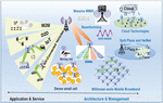
5G will become a prominent wireless infrastructure provider by satisfying diverse needs [1–5]. Both 5G and B5G wireless networks are linked to a lot of different other networks. Having the ability to partition physical network resources into logical slices, as well as massive connectivity, increased data throughput, and low latency, makes 5G more reliable. By increasing transmission speed or channel capacity, wireless users may access data, programs, and remote applications with extremely low latency. Smartphones, laptops, and other gadgets will rely less on internal memory and data collection. Due to cloud computing, certain tasks will not require many central processing units (CPUs). Figure 1 provides a simplified view of the 5G network architecture [6, 7]. The latency of a 5G connection is only 1 ms, while it was 200 ms for 4G. Remote actions may now be performed in real time thanks to wireless communication. The Internet of Things (IoT) is a promising and growing technology that is changing the world because of how many things can connect to it. To ease communication between networked devices, the IoT leverages the internet to regulate those with limited power. The idea and goal of IoT is to allow less latency and high reliability from end to end. Quality of service (QoS) in healthcare is conceivable with 5G Internet of Things (5G-IoT) because of its lowered latency and rise in sensors, for example. With the help of 5G networks, IoT systems will be able to connect single-point solutions and sensors to keep an eye on whole processes. These procedures may vary from research and development all the way to the conclusion of the product’s lifetime. The IoT with B5G and 5G wireless network integration is depicted in Figure 2 [8–10].
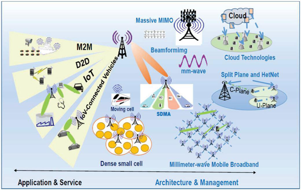
Figure 1 The schematic representation of the 5G wireless network.
In addition, OFDM is a widely used orthogonal modulation scheme. In OFDM, the wideband channel is subdivided into narrowband channels to reduce inter symbol interference (ISI). These subchannels adhere to the orthogonality property, but in the event of a significant Doppler shift, their orthogonality will vanish. Furthermore, multiple-input multiple-output (MIMO) diversity techniques enhance wireless data speed and end-to-end reliability. In the work [11], a novel MIMO-OFDM scheme is proposed, which presents fast data transmission rates, minimal out-of-band (OOB) emissions and a low peak-to-average power ratio (PAPR). Doppler spread is inherent in a high-velocity mobile environment and may mitigate the sub-carrier orthogonality, lowering signal detection effectiveness. PS priori channel knowledge influences CSI detector performance [12–14]. If there is no prior knowledge of the CSI, the CSI estimation is assumed to be imperfect. Immediately after getting the perfect knowledge of the CSI, CSI detectors are no longer required. The performance of OFDM systems is extremely sensitive to the techniques used for CSI estimation and signal identification. Consequently, a lot of work has gone into developing effective channel estimations and reliable signal detection schemes (see [15, 16] and references therein).
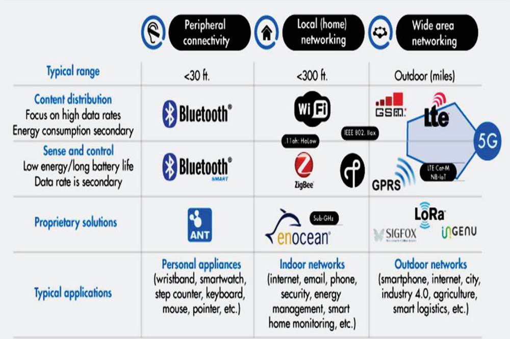
Figure 2 IoT with B5G and 5G wireless network integration.
Figure 3 Relationship between the AI, ML and DL.
1.2 Literature Survey
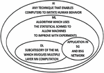
Artificial intelligence (AI) and machine learning (ML) enabled wireless networks to have already shown their impact in several recent 5G examples, including 5G network slicing [17–19], virtual reality (VR) and augmented reality (AR) [20, 21], big data analytics, mission-critical communications [21], and the massive IoT [22]. ML algorithms may replace traditional software with long rule lists. ML reduces the expensive process of hand-engineering features by using automatic feature extraction. Figure 3 shows the high-level link between AI, ML, and DL. In the work [23], the authors focus on ML-based B5G solutions. The work is organised according to the various kinds of ML algorithms to apply ML to 5G and B5G wireless networks. Further, the potential schemes are analysed for ML’s support of each 5G network requirement, emphasising their distinct use cases and rating their pros and cons for network operation. Furthermore, prospective B5G characteristics are listed to inspire further study on how ML might bring B5G to life [24–26]. LSTM is a specialised recurrent neural network (RNN) architecture with powerful modelling capabilities for long-term dependencies, allowing it to discover the connection between current and historical data. For this reason, mathematical modelling of 5G wireless networks is challenging owing to multipath propagation. Both DNNs and RNNs are examples of ML approaches that might be used to model the characteristics of the 5G wireless channel. DNN-based approaches do not need a model that can be solved mathematically, and it is easy to fix flaws like these. Loss estimation in a changing wireless channel presents a regression issue [27]. LSTM type DL architecture detects and predicts time series events with variable-sized delays [28, 29]. It is recommended to utilise a Bi-LSTM to address the issues with the LSTM. The authors of work [30] use an LSTM-based neural network (NN) to train the coefficients of a fading channel. When the cyclic prefix (CP) is removed and a limited number of pilots are used, the NN scheme proved to be superior to the more conventional LS and MMSE estimation systems. Based on the 5G tapped delay line “type C” model, the authors of the paper [31] claim that the Bi-LSTM technique reduces channel estimation error and BER in a MIMO-OFDM system considering the multipath propagation scenario. In this research, the Bi-LSTM channel estimation technique is used to the in single-input single-output (SISO) wireless communication system to enhance BER performance with reduced PS and no CP. The primary problems with signal estimation and channel characterisation in B5G wireless communication systems are handled by the improved NN schemes.
Many copies of a signal being delivered may lead to communication interference and a wide range of delays reaching the receiver due to multiple channels carrying the signal. This kind of interference may be mitigated by using the OFDM technique. Using the optimal signal detection algorithms and channel estimations improves multicarrier wireless system performance. This study uses Bi-LSTM-based DL to estimate the channel in multipath scenarios. CSI estimate is important for 5G and B5G systems [32]. Several CSI estimation algorithms exist. 5G wireless communications contain innovative techniques that need high processing complexity and are thus unsuitable. The primary problems with signal estimation and channel characterisation in B5G wireless communication systems are solved by the improved NN techniques. Communication interference, in the form of delay dispersion, is brought about by the considerable number of copies of a transmitted signal that arrive at the receiver through different channels. The OFDM scheme may mitigate these undesirable interference consequences. The next stage is to integrate an LSTM network with a convolutional neural network (CNN). In addition, the offline-online two-step training scheme has been modified, enabling more accurate predictions using real-world 5G wireless networks. Under the independent and identically distributed (i.i.d.) frequency flat doubly selective fading channels, the authors’ work [33] proposes an online DL-based CSI estimation technique. In addition to using previous channel estimates with well-chosen inputs, the DNN may use pilots and received signals to extract additional properties. The DNN may use LS estimation to boost channel estimation efficiency. Before monitoring a dynamic channel online, the DNN must learn to utilise simulated data offline. A pre-training strategy is created to improve the DNN’s initial settings, utilising many training epochs to reduce random initialization performance loss. The proposed solution uses DL’s learning and generalisation skills without channel data knowledge. It is more ideal for 5G networks with channel modelling ambiguities or time-varying fading links, such as high-mobility vehicle networks, cooperative cognitive relaying, device-to-device (D2D), machine-to-machine (M2M), and molecular communication systems [55–58]. In the work [57], the authors demonstrated that the node mobility has led the channel to lose its frequency flatness. Simulation and numerical findings reveal that the proposed DL-based estimator is more effective and robust against time selectivity. Recent interest has focused on DL physical layer applications. In [34, 35], a DL-based channel estimator is analysed for frequency-flat Rayleigh fading with temporal variations. The proposed receiver has been trained and evaluated using a DL algorithm. The proposed DL-based estimator is capable of dynamically tracking the channel status even without prior knowledge of the CSI. The simulation results demonstrate that the proposed NN estimator achieves better MMSE performance than both state-of-the-art DL-based designs and more conventional schemes. The DL-based estimator shows robustness with different pilot densities. The authors examine CSI estimation and present a DL-based channel estimate technique for real-time fading channel coefficients. After establishing several basic factors that impact a fading link’s CSI, the authors generate a data sample with feature and CSI information. Then, a DL approach combining LSTM and CNN is proposed. The CNN-LSTM hybrid algorithm performs superior to conventional DL-based approach. The purpose of the work [36] is to develop a DL Bi-LSTM RNN based CSI estimator for 5G OFDM systems.
The proposed estimator makes use of both online and offline techniques for training and practical use. Even though LS estimation is easy and less expensive, it has large channel estimate errors. The authors of [43] said that DL could be used to evaluate the perfect CSI. The research used the cross-entropy function, sum of squared errors (SSEs), and mean absolute error (MAE) as loss functions. In addition to the three layers of classification, the study used the root mean squared propagation (RMSProp), Adadelat, and SGD optimization methods. By using the proposed channel estimator, the efficacy of each classification layer is evaluated. Channel estimation and detection for OFDM wireless systems using feedforward DL NNs are developed in this study [37]. The suggested method has been shown to be more effective than the standard MMSE estimation method when anticipating the unknown effects of 5G networks. In [38], an online estimator for doubly selective channels using feedforward DL NNs is suggested. All the analysed works agree that the suggested estimate is superior to the industry standard MMSE estimator. In [39], a CNN DL estimator in a single dimension is investigated. Comparing the proposed estimator with MMSE, LS, and feedforward NN receivers for different complicated modulation schemes, the authors find that the proposed estimator performs better in terms of BER and mean square error (MSE). The suggested estimator has been shown to be superior to the conventional receivers. The online pilot assisted 5G system is analysed in the works [40, 59–64]. When there are few pilots and the initial channel data is unknown, the proposed estimate outperformed the LS and MMSE estimators, according to the contrasting study. The researchers in this work [41] used an artificial neural network (ANN) that had been optimized using a genetic algorithm to develop a CSI estimate. It is suggested that a specialised estimator be used in space time block code (STBC) MIMO-OFDM communication systems. The proposed estimator performed similarly to the LS and MMSE estimators at low SNRs, but it outperformed them both in terms of BER at high SNRs. In the study [53], the online DL-based CSI system is used to explore the DL LSTM method. To facilitate data recovery, the proposed estimator is first trained offline using simulated data sets. Then, it is deployed in real time propagation scenario while monitoring fading channel characteristics.
In the works [42, 43, 59, 60], the authors have proposed a CSI estimate for OFDM systems using ANN and performed a comparison analysis utilising three different DL optimization procedures to assess the estimator’s performance at each, assuming sparse multipath fading channel conditions. The recommended estimator outperformed matching pursuit-based and orthogonal matching pursuit-based estimators while requiring less computational effort. LS estimation is simple and less expensive, but it has large channel estimate errors. In the work [43], the authors suggest that the DL could be used to estimate LS channels. This study looks at 5G MIMO with Doppler spread and inaccurate channel estimates. As shown by the numerical findings, the suggested DL-assisted channel estimation technique is superior to the existing methods. As an alternative to using CNN, the authors suggest using Bi-LSTM as a CSI estimator. Given the smaller number of PS, the authors in the work [44] proposed a non-CSI channel estimate. The authors have proposed the data driven Bi-LSTM channel detector and estimator and it can significantly examine, classify, and recognize, and understand the statistical characteristics of wireless channels affected by ISI, electromagnetic interferences, co-channel interference (CCI), inter-user interference, self-interference, and others [44]. Despite the variety of DNN topologies, most research and implementations only use the “log” loss function [45]. This paper proposes two loss functions, MAE, and SSE, for coping with random channel statistical properties and constrained pilot densities. Bi-LSTM performance measures are compared to LS and MMSE CSI estimators. The Bi-LSTM-based estimator is superior to the LS and MMSE estimators and provides MMSE-like performance for large and low pilot numbers. The proposed estimator enhances OFDM wireless communication systems’ transmission data rates for a limited number of pilots. This article discusses the role that DL can play in overcoming challenges to autonomous 5G and B5G systems.
The main contribution of the paper is given below,
• Considering the tapped delay line type C (TDL-C) fading channel model, we build a 5G MIMO-OFDM network considering the Bi-LSTM DL scheme. It has been assumed that the proposed NOMA receiver does not have prior knowledge of the CSI and that the data symbols that are sent should include pilot signals to figure out the fading channel coefficients.
• In this work, cross entropy, MAE, SSE, and mean bias error (MBE) loss functions are given to produce the robust and precise channel estimator under Rayleigh fading channel conditions considering the limited number of PS.
• The proposed NOMA receiver is compared to the conventional MMSE and LS estimators. From the simulation results, the Bi-LSTM-based estimator is superior to both the LS and MMSE estimators, for both a small and substantial number of PS. The proposed estimate makes OFDM’s data transmission rate better because it works better when there are fewer pilots.
• The suggested channel estimator makes 5G OFDM systems work better overall, and when only a few pilots are used, it works better than the other estimators we looked at.
• We present a DNN for channel estimation. The DNN-based channel estimation does not require prior knowledge of the CSI. The DL-based channel estimation method trains a NN on a frequency- and time-selective fading channel with the help of LS channel estimations.
The work is organized in the following manner: In Section 2, the 5G-OFDM signal and channel model are analyzed, as well as a variety of receiver types. Further in Section 3, the Bi-LSTM-based CSI detection and estimation technique is presented, along with the offline and online training schemes. In addition, the loss function expressions are given in this section. The simulation results are presented in Section 4, and the article is concluded in Section 5.
2 Signal and Channel Model
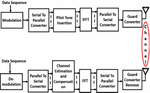
In this work, we examine the 5G MIMO-OFDM communication system, which is shown in Figure 4 [31]. Since the number of antennas on the transmitter (Tx) and the receiver (Rx) are and , respectively. So, the MIMO fading channel’s diversity order is equal to .
2.1 OFDM Transmitter
The modulation block encrypts and encodes, as seen in Figure 4. This block converts bits to symbols. The data sequence is mapped to the numbers of quadrature amplitude modulation (QAM) constellation symbols for encryption. We consider that the data is transmitted in the signalling intervals. The data vector is represented by and it is combination of all the QAM symbols in signalling time ; , expressed as [30–32],
| (1) |
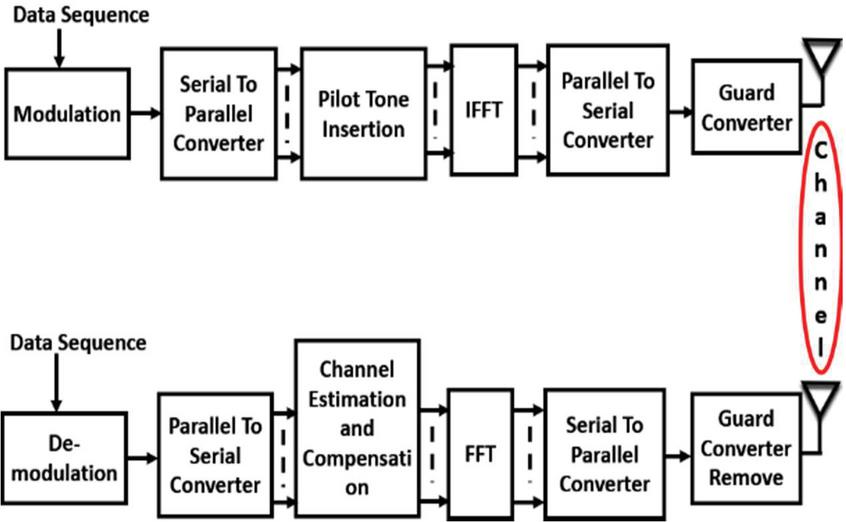
Figure 4 OFDM system model.
After the modulation block’s encoded data has been received, it is separated into vectors that correspond to the transmit antennas, as shown in the expression below,
| (2) |
The serial to parallel converter block is then used to convert the resultant signal vector to the parallel data vector. For channel estimation purpose, the signal vector is inserted with PS and the resulting signal vector is represented as, . The PS-inserted signal vector, denoted by is in the frequency domain; however, in order to convert it to the time domain signal vector, denoted by , an inverse fast Fourier transform (IFFT) algorithm is used. The time domain signal is expressed as,
| (3) |
ISI is a key problem for the MIMO-OFDM system; hence a CP has been inserted to reduce its effects. In the absence of guard bands in the OFDM system, a CP with a length of is employed in place of a guard interval. After CP insertion the signal vector is expressed as,
| (4) |
Where is the length of the fast Fourier transform (FFT). So, the signal vector has a length of , and it is generated by appending the last data symbols of to the beginning of the symbol as a CP.
2.2 5G Channel Modelling
The research [78] describes the 5G channel concept for 0.5 to 100 GHz. The fading channel models contain multi-path and Doppler shift phenomena, which cause frequency-selective and time-selective fading. In published works [30–32, 78], the TDL-C model has been considered for the non-line of sight fading channel from 0.5 to 100 GHz [33] with Rayleigh distributed fading links. According to the Jakes model, the power spectral density of each channel tap is expressed as [30–34],
| (5) |
The maximum value of the Doppler frequency in Hz is represented as and it is expressed as, , for a given speed (m/s) and a carrier frequency (Hz). The term represents the light speed. Since the inverse Fourier transform of the power spectral density is autocorrelation function (ACF) expressed as [30–34],
| (6) |
where represents the zeroth order Bessel function of the first kind. Since the time changes at every instant, the time index is discrete, and the discrete time ACF is written as [31],
| (7) |
The total symbol time is represented as and the term represents the time index. Let represents the time selective fading channel’s impulse response from the Rx antenna to Tx antenna. The multipath tap delay is represented by and is expressed as [30, 31],
| (8) |
Where the discrete amplitude of the resolved amplitude is represented by . Due to the relative motion between the Rx and Tx we are getting the doppler frequency, represented as . The discrete value of the doppler frequency is given as [30, 31], , where represents the relative velocity in discrete time and represents the discrete time phase shift of all the multi path components arriving in the tap. The received signal vector at the Rx after propagating over the time selective and frequency selective 5G channel may be expressed in (9) [30–32] by using the expression given in (8) and the signal that is broadcast in the expression (4).
| (9) |
where is expressed as, The AWGN noise vector is random process represented as . Each noise sample in the noise vector are i.i.d. random variables modelled as , i.e., circular shift with zero average value and spread around the mean is equal to . Using the formulation provided in (9), the fading channel coefficients can be easily estimated and evaluated the end-to-end OP and SER performance as given in the next subsection.
2.3 OFDM Receiver
At the Rx side the CP has been removed from the signal and the resulting signal vector is The length of the signal vector is . The signal is in serial form and the serial signal vector is converted to the parallel data. The time domain signal is converted to the frequency domain signal , represented as,
| (10) |
PS which are inserted for the channel estimation are extracted from the frequency domain signal and since the resulting signal is passed to the equalizer for removing the effect of the ISI. After equalization, the resulting parallel data vector is converted to the serial data vector. The serial data vectors are converted to the bit sequence by employing the demapping scheme in demodulation block.
3 LS and MMSE Channel Estimation
Perfect detection and estimation of the fading channel coefficients need the receiver to know the CSI in real-time propagation, particularly in time-selective fading channel scenarios. As such, PS-assisted CSI estimation relies heavily on multiplexing PS into the data stream. Frequency- or time-domain PS is dispersed using OFDM frames.
3.1 LS Detection Technique
The LS scheme approximates solutions in over-determined networks, which have more equations than unknowns. LS aims to minimise the cost function, represented as, . LS channel estimation locates the channel calculation to minimise the cost function, as expressed below,
| (11) |
The symbol stands for the conjugate transpose, while and stand for the signal being sent and the signal being received, respectively. Let is the 1st derivative of the cost function with respect to and putting equal to zero, as expressed below,
| (12) |
Considering , LS channel estimation is expressed as,
| (13) |
For each narrowband subchannel, the LS channel approximation is given below,
| (14) |
The LS method is straightforward to use, however it does not work well when there is node mobility, i.e., time varying fading channel conditions, expressed below,
| (15) |
We can evaluate the value of the weight by further minimizing the expression given in (15). Let the estimated value of the channel matrix is represented as and the exact value of the channel matrix is given as . The difference between the true value and the expected value of the channel matrix is given as, . Where represents the error matrix. It can be readily seen that the and the LS channel estimate is orthogonal with each other. The inner product between the and is expressed below,
| (16) | ||
Where the is the ACF between the matrix and . Further mathematical manipulation leads to,
| (17) |
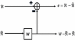
The schematic representation of the conventional MMSE receiver is given in Figure 5. Using the weight matrix given in (17), the MMSE channel estimation is given below,
| (18) | ||
| (19) |
Where represents the variance. It can be shown that, despite its complexity, the MMSE estimator outperforms the LS estimator significantly.
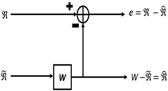
Figure 5 The schematic representation of the MMSE receiver.
4 Analysis of Bi-LSTM Based CSI Estimation
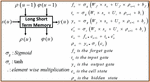
The fading channel coefficients in a 5G network are estimated using Bi-LSTM scheme. The Bi-LSTM network is the result of combining two RNN networks. This algorithm ensures that networks are always have knowledge of both the present and the prior sequences. Since there are two hidden layers and a two-way mechanism in place, we may concurrently store information from the past and the future. In reverse, LSTM is an RNN that can remember what will happen in the future. Inputs and applications often follow a sequential pattern. The interdependencies between them provide crucial insight into how they should be dealt with. RNNs, which can simulate the passage of time, perform well in such settings. The main concern of the RNN scheme is the vanishing gradients. When the gradient is too small, parameter changes can be neglected. Long data sequences are exceedingly difficult to train. Bi-directional RNN is an exact reproduction of the RNN processing sequence since it performs analyses on inputs in both the forward and backward directions. Now, an RNN with both forward and backward capabilities may potentially anticipate future events. LSTM and gated recurrent units (GRU) are two RNN designs that are widely used. LSTM is superior to RNN when considering the long-term dependencies. The Bi-LSTM is a well-liked choice for natural language processing (NLP) applications. The introduction of feedback connections sets LSTM apart from conventional feedforward NNs. It is capable of handling data sequences in their whole, not just isolated instances. The conventional LSTM components are the cell state, hidden state, forget gate, output gate and gate. Figure 6 shows a graphical representation of the input/output pairs for a single time step in an unrolled LSTM. The LSTM network receives the input denoted by the letter [77]. This input might be the output of a CNN, or it could simply be the input sequence itself. The inputs for the LSTM at the preceding time step are and . The output of the LSTM for this time step is denoted by the symbol The LSTM is also responsible for the generation of the and values, which are then used by the subsequent time step LSTM. It is important to take note that the LSTM equations also produce and . These are for the internal consumption of the LSTM and are utilized for producing and .
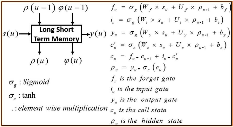
Figure 6 LSTM cell and various expressions [77].
4.1 The Proposed Bi-LSTM Based CSI Information
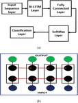
The weights and biases of the recommended estimator are enhanced by using SGD [46] and CO techniques. SGD optimization schemes have gained prominence in 5G-IoT. Traditional SGD is different from SGD [47, 48]. With the SGD scheme, the rate at which weights are adjusted (the “learning rate,” or “alpha”) is constant. The SGD optimization, which uses the cross entropy, MAE, cross entropy for the mutually exclusive class, and SSE loss functions, is used to train the proposed estimator. Simply put, a loss function is a metric for evaluating how effectively a prediction model can predict the statistical characteristics of a channel, considering the low number of PS. The scheme is adjusted to get the optimal value by minimising the loss function once the learning problem has been transformed into an optimization problem. Input sequence, Bi-LSTM, fully linked, softmax, and output classification make up the five layers that make up the proposed scheme. A NN layer is used as part of the implementation of the Softmax layer [49, 50]. This layer comes before the output layer. Both the output layer and the Softmax layer need a certain number of nodes to function properly. A Bi-LSTM layer is used whenever there is a need to uncover the long-term bi-directional correlations that exist between different time steps in a time series or sequence of data. Bi-LSTM is a sequence processing model, and it comprises two LSTMs: one that processes the input in a forward way, and the other that processes it in a backwards fashion. The quantity of information that can be accessed by the network is effectively increased using Bi-LSTMs, which in turn improves the context that can be accessed by the algorithm. The amount of data that the network has access to is significantly increased by Bi-LSTMs, which helps the algorithm comprehend the context. The input field could only contain 255 characters. The fifteen hidden units of the Bi-LSTM layer show the last component of the sequence. The four classifications are defined by a fully connected layer of size five, a softmax layer, a classification layer, and a classification layer only. The structure of the proposed estimator is shown in Figure 7(a) [51]. Figure 7(a) can be compressed into a single block as Figure 7(b) [52].

Figure 7 (a) Bi-LSTM NN and (b) Bi-LSTM cell.
4.2 Investigation of Bi-LSTM Channel Estimator
4.2.1 Offline investigation
Although DNNs are the most advanced 5G wireless network architecture, training them is a computationally complex, resource-intensive, and time-consuming process. GPUs are the most useful hardware for training a DNN [34, 35]. Due to the presence of a massive number of Bi-LSTM-NN parameters, including weights and biases, that must be updated during training, the proposed CSI estimate is time-consuming to train, and offline training is a good option. With the ability to perform AI computing operations in parallel, DL graphics processing units (GPUs) have the potential to drastically cut down on training times. When evaluating GPUs, you should think about how many you can connect, the availability of the software that goes along with it, licencing, data parallelism, memory utilisation, and performance. Since the suggested CSI estimate requires a long training period and several Bi-LSTM NN parameters, including biases, and weights, must be adjusted during training, it is recommended that it be done offline.
4.2.2 Online investigation
In the online implementation, the transmitted signal will be mitigated using the trained CSI estimate [36]. During offline training, a random data set for learning is generated for a single sub carrier. Frame every frame, OFDM merely sends a single pilot and data symbol over the channel. The received data are utilised to reconstruct the OFDM signal using frames with varying degrees of channel estimate uncertainty. All classical estimators depend largely on mathematical fading channel models based on Gaussian statistics since these models are tractable and guarantee that the estimator will be linear, stationary, and linear in time. Researchers have developed several fading channel models that closely match the actual channel parameters, even though it is challenging to account for additional CSI errors and unknown surrounding effects using precise channel models. These models of fading channels may be used in conjunction with channel modelling to provide high-quality, practically applicable training datasets [36]. Using the third-generation partnership project (3GPP) TR 38.901 V16.0.0 standard channel model [37, 38], this research determines the end-to-end OP and SER performance of 5G wireless networks and the cumulative fading channel distribution of 5G NOMA. Several methods exist for determining the loss function, which is the deviation between the estimator’s results and the input values. The activation functions in matrix laboratory (MATLAB) 2021 include binary step function, Sigmoid, Leaky rectified linear activation function (ReLU), and rectified linear activation function (ReLU) function [39]. The loss functions Cross entropy, MAE, SSE, and MBE are expressed as,
| Cross Entropy | (20) | |
| MAE | (21) | |
| SSE | (22) | |
| MBE | (23) |
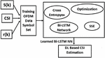
In (20) represents the OFDM symbol for the class, and denote the class number and sample number, respectively. Additionally, represents the Bi-LSTM based CSI channel estimation for sample belonging to class . Figure 8 shows how to build a training dataset and use offline DL to get a trained CSI estimate.
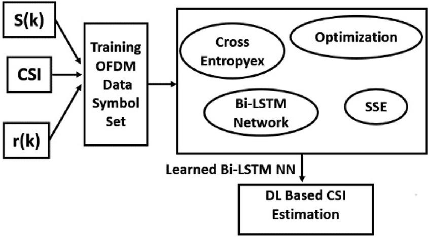
Figure 8 The Bi-LSTM-NN-based CSI estimator’s offline DL procedure and generation of an OFDM complicated data set are both based on Bi-LSTM.
5 Simulation Results and Discussions
Here, in this section, numerical and simulation results have been demonstrated for analysing the end-to-end system performance of the Bi-LSTM based 5G-OFDM system. The primary drawback of traditional estimating methods is the need for CSI. Prior CSI expertise is not necessary for our simulations. The most reliable iteration of the suggested CSI estimate is produced by considering different loss functions and optimization techniques like CO and SGD. The simulation software’s Python 3.9.2, MATLAB 5G Toolbox, and CVX are being considered for use in the simulation and optimization processes. The Bi-LSTM SGD-based CSI estimator is suggested in the study [53], which also evaluated the BER performance for low, medium, and high SNR regimes, respectively. A priori uncertainty in the statistics of the applied fading model is assumed and considered for all simulations. Additionally, to create the most reliable CSI estimation, the SGD optimisation technique is employed to train the suggested estimator while employing various loss functions. Table 1 shows Bi-LSTM, LSTM, and training possibilities.
Table 1 Bi-LSTM layer and LSTM layer NN training parameters
| Parameter | Value |
| Length of the input vector | 300 |
| Length of the Bi-LSTM layer | 40 neurons (hidden) |
| Length of the LSTM layer | 40 neurons (hidden) |
| Size of the fully connected layers | 6 |
| Loss Functions | MAE/L1 Loss, MBE, SSE |
| Mini Batch Size | 1500 |
| Total number of Epochs | 1500 |
| ML algorithm | SGD |
| Number of trainings OFDM symbols | 10000 OFDM frame |
| Number of Validation OFDM symbols | 5000 OFDM frame |
| Algorithm test data size | 15000 OFDM frame |
Table 2 contains the fading channel characteristics and the model for the OFDM system. The proposed channel estimator’s performance is compared over several scenarios, including PS values of 8, 16, and 72 and the PyTorch mean absolute error (L Loss Function) (MAE/L Loss), MBE, and SSE loss functions. For all simulations, the SGD optimization scheme is employed.
Table 2 OFDM model system parameters
| Digital Modulation Technique | QAM |
| Carrier frequency | 2.6 GHz |
| Number of multiple paths | Forty hidden neurons |
| Length of the CP | 20 |
| Number of subcarriers | 72 |
| Number of pilots | 8, 16, and 72 pilots |

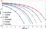
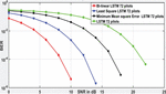
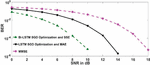
Figure 9 Performance comparison of BER and SNR in dB employing 8, 16, and 72 pilots while considering SGD optimization, SSE, and MAE/L1 loss functions.
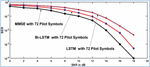
Figure 9 shows that when there are enough PS (72 or more), the proposed Bi-LSTM SGD estimator outperforms the Bi-LSTM SGD, LS, and MMSE estimators in the intermediate and higher SNR regimes. The Bi-LSTM-MAE/L estimator outperforms the LS estimator in the 0–16 dB SNR range, while the LSTM-SGD estimator outperforms both in the 0–18 dB SNR range. The MMSE estimator agrees with the Bi-LSTM-MAE/L and LSTM-SGD estimators for the [0 to 12 dB] and [0 to 6 dB] SNR ranges, respectively. In the absence of these SNR bounds, the MMSE estimator outperforms the Bi-LSTM-MAE/L and the LSTM-SGD estimators. From 0 to 18 dB, Bi-LSTM MAE/L outperforms LSTM SGD. The curves show that at SNR values between 0 and 8 dB, the performance of the Bi-LSTM SGD and LSTM SSE estimators is quite consistent with the performance of the MMSE estimator. Bi-LSTM SGD and LSTM SSE are outperformed by the LS estimator by over 16 dB and over 12 dB, respectively. However, MMSE performs better than the Bi-LSTM SSE and LSTM SSE estimators by a margin of more than 8 dB. The BER performance of the proposed estimator is analysed for 6, 10, and 72 numbers of PS. The considered loss functions are cross entropy, MAE, SSE, and MBE loss functions. For minimising the BER, the CO optimization method using CVX software, and the SGD optimization method are considered. Considering the 72 PS, it is clear from the curves in Figure 10 that the proposed Bi-LSTM cross entropy scheme outperformed the LSTM cross entropy, LS, and MMSE estimators for low, medium, and high SNR regimes. Figure 11 shows that when the pilot number is seventy-two and the MAE loss function is utilised, the Bi-LSTM MAE estimator performs better than the LS estimator. Also, the LSTM MAE does better in the range of 0–18 dB SNR. Also, the performance of the MMSE estimator and the Bi-LSTM MAE estimator are remarkably close for the ranges 0 to 15 dB SNR and 0 to 6 dB SNR. Over specific SNR limits, MMSE outperforms Bi-LSTM and LSTM MAE. A Bi-LSTM performs better than a single-directional LSTM in terms of MAE. The LSTM MAE has a range of 6–20 dB.
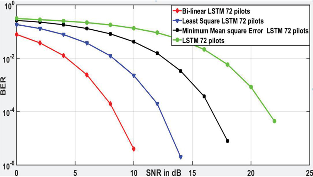
Figure 10 The BER performance comparison between the Bi-LSTM and other conventional estimators for 72 numbers of PS.
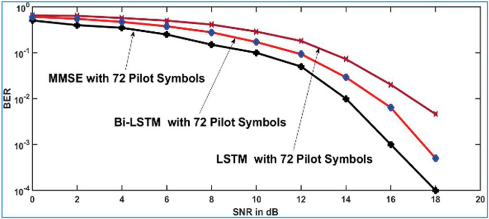
Figure 11 BER comparison of 72 pilots between the suggested, LSTM, and conventional estimators.
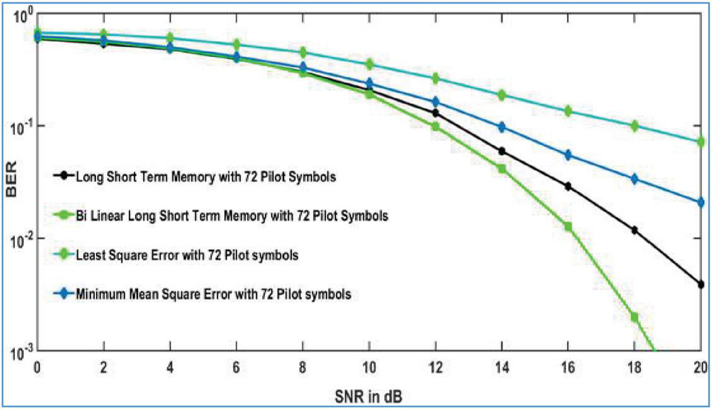
Figure 12 Bi-LSTM and other channel estimators’ BER performance with 72 pilots and SSE loss function.
Figure 12 shows that when the SSE loss function is used, the Bi-LSTM SSE and LSTM SSE estimators perform better than the MMSE estimator in the low SNR region [0–10 dB]. The Bi-LSTM SSE and LSTM SSE estimators perform worse than the MMSE estimators starting at 10 dB. The Bi-LSTM SSE is exceeded by the LS estimator by 18 dB. Together, LSTM’s squared error sum is greater than LSTM’s squared error sum by 10 to 20 dB. The LS underperforms MMSE because the estimation technique does not consider prior knowledge of the CSI. With a large enough number of pilots, MMSE’s improved performance is due to the application of second-order statistics. Figure 13 gives the performance comparison between the proposed estimator with other conventional channel estimators for various loss functions considering the 72 PS. MMSE and Bi-directional cross entropy LSTM provide near BER performance in all SNR regimes. This fraction is same whether utilising 0 to 10 dB SNR, two-way LSTM (cross entropy), LSTM, and MMSE.
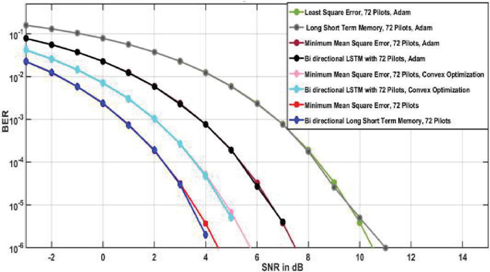
Figure 13 BER comparison of several receiver estimators utilising 72 pilots, the SGD learning method, and the loss functions cross entropy, MAE, and SSE.
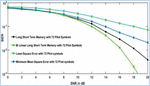
Figure 14 compares the performance of the Bi-LSTM (cross entropy), the LSTM (cross entropy), and the traditional channel detection and estimation schemes over a range of SNR values and loss functions. In comparison to both the LSTM (cross entropy) and traditional estimators, the Bi-LSTM (cross entropy) shows substantial improvement, as shown by the graphs. The suggested Bi-LSTM estimators (cross entropy) perform comparably in the 0–10 dB SNR range. The suggested estimator outperforms both the Bi-LSTM MAE, which is trained by the lowest of the average absolute error loss functions, and the two-way LSTM cross-entropy estimator, which is trained to minimise the cross-entropy loss function by 10 dB. The curves demonstrate how useful Bi-LSTM-based estimators may be in scenarios when there are a limited number of PS and a priori uncertainty about the CSI. The curves show how testing multiple loss functions in DL may help select the optimum layout estimator. Further, it is demonstrated that the proposed estimator is superior to one that uses a fixed number of PS and is sensitive to the prior knowledge of the CSI. Furthermore, plots demonstrate the need for simulations considering the various loss functions to find the optimal structure for each estimate in the DL procedure. Like the Bi-LSTM (cross entropy) performance at 72 pilots, the Bi-LSTM error performance at 10 PS is also comparable. Therefore, the presented estimators with a few PS are recommended for usage in 5G OFDM wireless communication systems to greatly enhance their data rate. Since the suggested estimator advocated employing a data-driven training approach, the fading channel statistics are insensitive to a priori knowledge of the CSI.
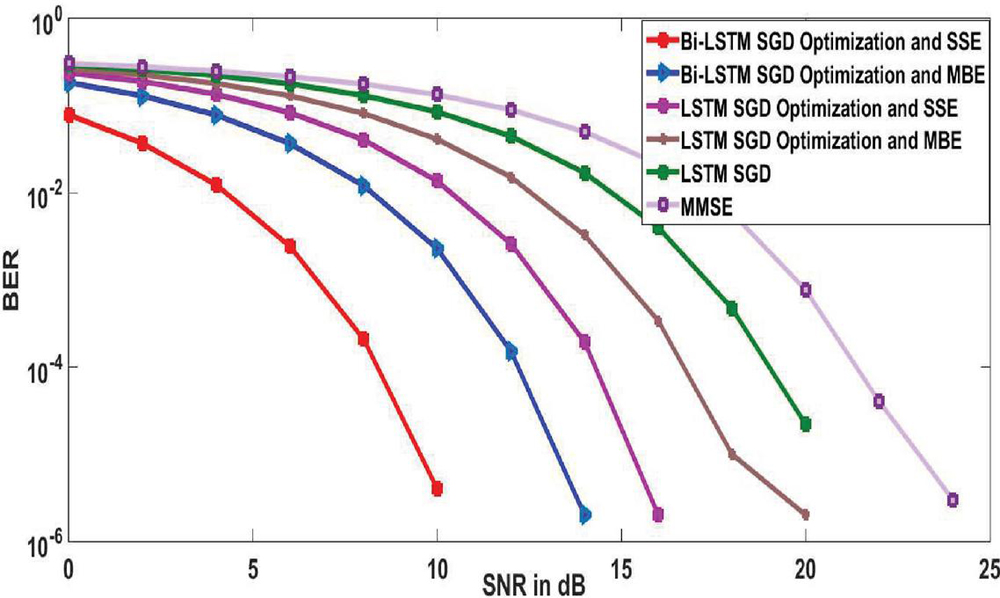
Figure 14 LS, MMSE, LSTM, and Bi-LSTM estimators with 8 PS utilising SGD learning and cross-entropy, MAE, and SSE loss functions.
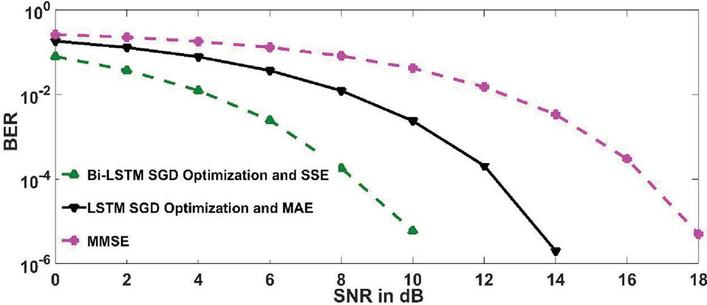
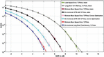
Figure 15 The BER performance of the proposed, LSTM, and traditional estimators was compared using four pilots and the SSE loss function.
Figure 15 shows the estimated values for LSTM (cross entropy), LS, and MMSE in 6 distinct PS. The suggested system further demonstrates the superiority of the two-way LSTM estimator over conventional estimators, which become ineffective at 0 dB. Moreover, the proposed two-way LSTM estimator is shown to be superior to LSTM. From 0 to 14 dB, LSTM (cross entropy) agrees with the LSTM, and at 15 dB, it becomes a two-way LSTM (cross entropy). Perform similarly to the recommended Bi-LSTM estimators for the 0–5 dB SNR range (cross entropy, medium absolute error, or squared error sum). The proposed two-way LSTM estimator outperforms the Bi-LSTM cross-entropy estimator by 10 dB in terms of squared error and is on par with the two-way LSTM MAE estimator in terms of SNR gain. Training loss curves provide an accurate measure of the DL NN training procedure’s success. Depending on the information provided by the loss curves, the user may determine whether to proceed with further training. For DL’s NN-based estimators, Figure 15 shows the losses for pilot numbers 72, 10, and 6 (cross entropy, MAE, and SSE). The results are highlighted and verified by the curves shown in Figures 11–15. The curves in the Figure 15 for the Bi-LSTM cross entropy and LSTM cross entropy estimators demonstrate their superiority over other estimators. Figures 13 and 14 show the BER performance of each DL NN-based CSI estimate, whereas Figure 15 shows the training loss curves for these estimates. When comparing the proposed estimators to other examined estimators, accuracy is utilised to describe how effectively each estimator gets the knowledge of perfect CSI. Accuracy is measured by dividing the number of correctly received symbols by the number of transmitted symbols. After training the proposed estimator with various parameters, we will test it on a fresh dataset. Further from Table III, we can observe each estimator’s accuracy in every simulated situation, furthermore it shows that the proposed Bi-LSTM-based estimator obtains accuracies between 98.61 and 100.
Table 3 Accuracy analysis for 72 pilot numbers
| Bi-LSTM | LSTM | MMSE | LS | |
| Cross entropy | 99.99 | 98.99 | 99.99 | 98.94 |
| SSE | 98.23 | 98.88 | 110 | 98.94 |
| MAE | 98.87 | 98.53 | 110 | 98.94 |
The alternative DL LSTM-based estimator performed between 97.88 and 99.99 percent accurately under the same test conditions as the original. The resulting BER performance is shown in Figure 14 to illustrate how the suggested estimator has learned robustly in response to the observed accuracies. Tables 1, 2, and 3 provide MMSE and LS results, respectively; these tables highlight the BER’s provided performance in Figures 12 through 14 and demonstrate that the accuracy of traditional estimators decreases noticeably when the number of pilots is reduced, as seen in Figures 15.
DL schemes are used to analyse large datasets, find statistical correlations and properties, construct feature-specified connections, and obtain new data sets. All 5G and B5G networks should take this into account. Feed forward transmission procedures dominate the complexity of all NNs, for example, LSTM and Bi-LSTM. The feed-forward pass computes the combined weights of the layers preceding the current one. When the errors are assessed using a feedback pass, the weights are revised accordingly. The LSTM’s computational complexity is given below,
| (24) |
stands for the weight matrix, for the number of outputs, for the number of hidden layers, for the number of inputs, for the number of memory cell blocks, and for the size of each block of memory [23]. The Bi-LSTM design consists of two LSTM NN sites and two routes of propagation (forward and backward). Hence, is used in Bi-LSTM. The computational complexity of Bi-LSTM is,
| (25) |
The amount of time spent in training is another indicator of complexity. The accuracy comparison between Bi-LSTM and LSTM layer is shown in Table 4. The used computer contains an Intel (R) Core i5-2400 processor running at 3.10–3.30 GHz and 12 GB of RAM. When compared to their Bi-LSTM counterparts, estimators based on LSTM need less time to analyse data. Because of this, their complexity is quite low.
Table 4 Layer and LSTM layer
| Seventy-two | Seventy-two | Seventy-two | Ten | Ten | Six | Six |
| Pilots | Pilots | Pilots | Pilots | Pilots | Pilots | Pilots |
| Bi-LSTM | LSTM | Bi-LSTM | LSTM | Bi-LSTM | LSTM | |
| Cross entropy | 99.99 | 99.99 | 99.80 | 98.90 | 99.78 | 98.90 |
| SSE | 97.23 | 99.88 | 99.23 | 97.85 | 97.23 | 98.80 |
| MBE | 97.87 | 98.10 | 99.87 | 98.54 | 97.87 | 98.81 |
6 Conclusion
In terms of BER and accuracy metrics, the LSTM DL based CSI, LS, and MMSE estimators outperform the Bi-LSTM receiver in a variety of simulated scenarios. For DL Bi-LSTM and LSTM-based estimators, it contains details on the computational and training time complexity. The proposed channel detection scheme is based on the DL approach. It is helpful for 5G and B5G systems because it can analyse vast volumes of data, find statistical dependencies and features, build correlations between features, and generalise the information obtained for new datasets. The suggested online pilot-assisted CSI estimator is the proposed DL Bi-LSTM. It outperforms traditional estimators and is robust to a limited number of pilots. In case of real time communication scenario where due to the doppler spread the fading channel coefficients are changing very rapidly (non-Gaussian or non-stationary channels), it is almost impossible to get perfect knowledge of the CSI. In these cases, the proposed Bi-LSTM estimate is better than both the traditional and the LSTM based CSI estimator. The proposed CSI estimator does better than traditional CSI estimators at low SNRs, especially for lower PS, and it works the same for both large and small pilot numbers. The proposed Bi-LSTM-based 5G system offers the most accurate predictions for 72, 10, and 6 pilots for all loss functions. The proposed LSTM and Bi-LSTM estimators are quite reliable, with a MAE between 97.61 and 99% and a sum of 72, 10, and 6 pilot error loss functions of 70%. There is much promise in both 5G and the next version of B5G. New, user-adjustable loss functions illustrated in two examples (MAE and SSE errors). The computational and learning challenges of the LSTM estimator are used to characterise its difficulty.
7 Future Scope
• Investigate the efficacy of the recommended estimator in terms of both its performance and its accuracy using a variety of research techniques, including as the Nesterov accelerated gradient, Momentum, Adam variant of gradient descent (AMSGrad), and root mean squared propagation (RMSprop).
• Examine the effectiveness of the suggested estimator in terms of both its performance and its accuracy by using various lengths and types of CPs. The research and development of robust loss functions via the use of robust estimators such as Geman-McClure, Cauchy, Redescenders, and Hampel.
• Cross entropy, MAE and SSE loss functions are used to examine the efficacy of the RNN, LSTM, and GRU based estimations for the 72, 10, and 6 pilots, respectively.
References
[1] Pandya S, Wakchaure MA, Shankar R, Annam JR. “Analysis of NOMA-OFDM 5G wireless system using deep neural network”, The Journal of Defense Modeling and Simulation, vol. 19, Issue 4, pp. 799–806, 2022. DOI: 10.1177/1548512921999108.
[2] R. Tiwari and S. Deshmukh, “Handover Count Based MAP Estimation of Velocity with Prior Distribution Approximated via NGSIM Data-Set,” in IEEE Transactions on Intelligent Transportation Systems, vol. 23, no. 5, pp. 4352–4361, May 2022, DOI: 10.1109/TITS.2020.3043888.
[3] Chaudhary BP, Shankar R, Mishra RK. “A tutorial on cooperative non-orthogonal multiple access networks”, The Journal of Defense Modeling and Simulation, vol. 19, Issue 4, pp. 563–573, 2022. DOI: 10.1177/1548512920986627.
[4] Ravi Tiwari, Siddharth Deshmukh, “Analysis and design of an efficient handoff management strategy via velocity estimation in HetNets”, Transactions on Emerging Telecommunications Technologies, vol. 33, Issue 3, e3642, March 2022. https://doi.org/10.1002/ett.3642.
[5] R. Tiwari and S. Deshmukh, “Prior Information-Based Bayesian MMSE Estimation of Velocity in HetNets,” in IEEE Wireless Communications Letters, vol. 8, no. 1, pp. 81–84, Feb. 2019. DOI: 10.1109/LWC.2018.2857805.
[6] M. Agiwal, A. Roy and N. Saxena, “Next Generation 5G Wireless Networks: A Comprehensive Survey”, IEEE Communications Surveys & Tutorials, vol. 18, no. 3, pp. 1617–1655, 2016. DOI: 10.1109/COMST.2016.2532458.
[7] Dankan Gowda V, Avinash Sharma, B. Kameswara Rao, Ravi Shankar, Parismita Sarma, Abhay Chaturvedi, Naziya Hussain, “Industrial quality healthcare services using Internet of Things and fog computing approach”, Measurement: Sensors, Elsevier, vol. 24, pp. 100517, 2022, ISSN 2665–9174, https://doi.org/10.1016/j.measen.2022.100517.K.
[8] Shafique, B. A. Khawaja, F. Sabir, S. Qazi, and M. Mustaqim, “Internet of Things (IoT) for Next-Generation Smart Systems: A Review of Current Challenges, Future Trends and Prospects for Emerging 5G-IoT Scenarios,” in IEEE Access, vol. 8, pp. 23022–23040, 2020. DOI: 10.1109/ACCESS.2020.2970118.
[9] X. Liu and X. Zhang, “Rate and Energy Efficiency Improvements for 5G-Based IoT with Simultaneous Transfer,” IEEE Internet of Things Journal, vol. 6, no. 4, pp. 5971–5980, Aug. 2019. DOI: 10.1109/JIOT.2018.2863267.
[10] Ahmed, Rizwan and Malviya, Anil Kumar and Kaur, Maninder Jeet and Mishra, Ved P., “Comprehensive Survey of Key Technologies Enabling 5G-IoT”, Proceedings of 2nd International Conference on Advanced Computing and Software Engineering (ICACSE) 2019, Available at SSRN: https://ssrn.com/abstract=3351007~or~http://dx.doi.org/10.2139/ssrn.3351007.
[11] M. H. Mahmud, K. Khaleduzzaman, S. Sarker and L. Chandra Paul, “Effect of Path Loss Models on Performance of 5G Compatible MIMO window-OFDM Systems”, International Conference on Smart Technologies in Computing, Electrical and Electronics (ICSTCEE), pp. 257–262, 2020. DOI: 10.1109/ICSTCEE49637.2020.9277121.
[12] Bhardwaj, Lokesh, Ritesh Kumar Mishra, and Ravi Shankar. “Investigation of Low-Density Parity Check Codes Concatenated Multi-User Massive Multiple-Input Multiple-Output Systems with Imperfect Channel State Information.” The Journal of Defense Modeling and Simulation, vol. 19, no. 3, pp. 539–50, July 2022. https://doi.org/10.1177/1548512920968639.
[13] T. Li, X. Hao, and X. Yue, “A Power Domain Multiplexing Based Co-Carrier Transmission Method in Hybrid Satellite Communication Networks,” in IEEE Access, vol. 8, pp. 120036–120043, 2020, DOI: 10.1109/ACCESS.2020.3005860.
[14] Ravi Shankar, Ritesh Kumar Mishra, “S-DF Cooperative Communication System over Time Selective Fading Channel”, Journal of Information science and Engineering, vol. 35, Issue 6, pp. 1223–1248, 2019. DOI: 10.6688/JISE.201911\_35(6).0004.
[15] Das, A.K., Pramanik, A., “A Survey Report on Underwater Acoustic Channel Estimation of MIMO-OFDM System”, In: Bhattacharjee, D., Kole, D.K., Dey, N., Basu, S., Plewczynski, D. (eds) Proceedings of International Conference on Frontiers in Computing and Systems. Advances in Intelligent Systems and Computing, vol. 1255, 2021. Springer, Singapore. https://doi.org/10.1007/978--981-15--7834-2\_69.
[16] Chitikena, Rajeshbabu, and P. Estherrani. “Time-Varying Analysis of Channel Estimation in OFDM.” Advances in Smart System Technologies, pp. 669–678. Springer, Singapore, 2021.
[17] N. Taherkhani and S. Pierre, “Centralized and Localized Data Congestion Control Strategy for Vehicular Ad Hoc Networks Using a Machine Learning Clustering Algorithm,” IEEE Transactions on Intelligent Transportation Systems, vol. 17, no. 11, pp. 3275–3285, Nov. 2016. DOI: 10.1109/TITS.2016.2546555.
[18] J. Kwak, Y. Kim, L. B. Le, and S. Chong, “Hybrid Content Caching in 5G Wireless Networks: Cloud Versus Edge Caching,” IEEE Transactions on Wireless Communications, vol. 17, no. 5, pp. 3030–3045, May 2018, doi: 10.1109/TWC.2018.2805893.
[19] Z. Chang, L. Lei, Z. Zhou, S. Mao, and T. Ristaniemi, “Learn to Cache: Machine Learning for Network Edge Caching in the Big Data Era,” IEEE Wireless Communications, vol. 25, no. 3, pp. 28–35, June 2018, doi: 10.1109/MWC.2018.1700317.
[20] A. Saeed and M. Kolberg, “Towards Optimizing WLANs Power Saving: Novel Context-Aware Network Traffic Classification Based on a Machine Learning Approach,” IEEE Access, vol. 7, pp. 3122–3135, 2019, DOI: 10.1109/ACCESS.2018.2888813.
[21] E. Bastug, M. Bennis, E. Zeydan, M. A. Kader, I. A. Karatepe, A. S. Er, and M. Debbah, “Big data meets telcos: A proactive caching perspective,” J. Commun. Netw., vol. 17, no. 6, pp. 549–557, Dec. 2015. https://doi.org/10.48550/arXiv.1602.06215.
[22] A. Imran, A. Zoha, and A. Abu-Dayya, “Challenges in 5G: How to empower SON with big data for enabling 5G,” IEEE Netw., vol. 28, no. 6, pp. 27–33, Nov./Dec. 2014.
[23] M. E. Morocho-Cayamcela, H. Lee and W. Lim, “Machine Learning for 5G/B5G Mobile and Wireless Communications: Potential, Limitations, and Future Directions,” in IEEE Access, vol. 7, pp. 137184–137206, 2019, doi: 10.1109/ACCESS.2019.2942390.
[24] F. Kadri, M. Baraoui and I. Nouaouri, “An LSTM-based DL Approach with Application to Predicting Hospital Emergency Department Admissions,” 2019 International Conference on Industrial Engineering and Systems Management (IESM), pp. 1–6, 2019. DOI: 10.1109/IESM45758.2019.8948130.
[25] Kaushik, S., Choudhury, A., Dasgupta, N., Natarajan, S., Pickett, L.A., Dutt, V., “Ensemble of Multi-headed Machine Learning Architectures for Time-Series Forecasting of Healthcare Expenditures”, In: Johri, P., Verma, J., Paul, S. (eds) Applications of Machine Learning. Algorithms for Intelligent Systems. Springer, Singapore, 2020. https://doi.org/10.1007/978--981-15--3357-0\_14.
[26] Batbaatar E, Ryu KH., “Ontology-Based Healthcare Named Entity Recognition from Twitter Messages Using a Recurrent NN Approach”, International Journal of Environmental Research and Public Health, vol. 16, pp. 3628, 2019.
[27] Thien HT, Tuan PV, Koo I, “Deep Learning-Based Approach to Fast Power Allocation in SISO SWIPT Systems with a Power-Splitting Scheme”, Applied Sciences, vol. 10, pp. 3634, 2020.
[28] L. Fernández Maimó, Á. L. Perales Gómez, F. J. García Clemente, M. Gil Pérez, and G. Martínez Pérez, “A Self-Adaptive Deep Learning-Based System for Anomaly Detection in 5G Networks,” in IEEE Access, vol. 6, pp. 7700–7712, 2018, doi: 10.1109/ACCESS.2018.2803446.
[29] M. Schuster and K. K. Paliwal, “Bidirectional recurrent neural networks,” in IEEE Transactions on Signal Processing, vol. 45, no. 11, pp. 2673–2681, Nov. 1997, doi: 10.1109/78.650093.
[30] Narengerile. Deep learning-based signal detection in OFDM systems. (https://www.mathworks.com/matlabcentral/fileexchange/72321-deep-learning-based-signal-detection-in-ofdm-systems), MATLAB Central File Exchange. Retrieved September 26, 2020.
[31] Le HA, Van Chien T, Nguyen TH, et al., “Machine Learning-Based 5G-and-Beyond Channel Estimation for MIMO-OFDM Communication Systems”, Sensors, vol. 21, pp. 4861, 2021.
[32] C. Luo, J. Ji, Q. Wang, X. Chen, and P. Li, “Channel State Information Prediction for 5G Wireless Communications: A Deep Learning Approach,” in IEEE Transactions on Network Science and Engineering, vol. 7, no. 1, pp. 227–236, 1 Jan.–March 2020. DOI: 10.1109/TNSE.2018.2848960.
[33] Y. Yang, F. Gao, X. Ma, and S. Zhang, “Deep Learning-Based Channel Estimation for Doubly Selective Fading Channels,” in IEEE Access, vol. 7, pp. 36579–36589, 2019. DOI: 10.1109/ACCESS.2019.2901066.
[34] Q. Bai, J. Wang, Y. Zhang, and J. Song, “Deep Learning-Based Channel Estimation Algorithm Over Time Selective Fading Channels,” in IEEE Transactions on Cognitive Communications and Networking, vol. 6, no. 1, pp. 125–134, March 2020. DOI: 10.1109/TCCN.2019.2943455.
[35] D Venkata Ratnam, K Nageswara Rao. “Bi-LSTM based deep learning method for 5G signal detection and channel estimation”, AIMS Electronics and Electrical Engineering, vol. 5, Issue 4, pp. 2021, 334–341, 2021. DOI: 10.3934/electreng.2021017.
[36] Essai Ali MH, Taha IBM., “Channel state information estimation for 5G wireless communication systems: recurrent NNs approach”, PeerJ Computer Science, vol. 7, pp. e682, 2021. https://doi.org/10.7717/peerj-cs.682.
[37] H. Ye, G. Y. Li and B. -H. Juang, “Power of Deep Learning for Channel Estimation and Signal Detection in OFDM Systems,” in IEEE Wireless Communications Letters, vol. 7, no. 1, pp. 114–117, Feb. 2018. DOI: 10.1109/LWC.2017.2757490.
[38] J. M. Kang, C. J. Chun, and I. M. Kim, “Deep Learning Based Channel Estimation for MIMO Systems with Received SNR Feedback,” in IEEE Access, vol. 8, pp. 121162–121181, 2020. DOI: 10.1109/ACCESS.2020.3006518.
[39] Ponnaluru, S., Penke, S. “Deep learning for estimating the channel in orthogonal frequency division multiplexing systems”, J Ambient Intell Human Comput, vol. 12, pp. 5325–5336, 2021. https://doi.org/10.1007/s12652-020-02010-1.
[40] Essai Ali MH., “Deep learning-based pilot-assisted channel state estimator for OFDM systems”, IET Communications, vol. 15, Issue 2, pp. 257–264, 2021. https://doi.org/10.1049/cmu2.12051.
[41] A. Sarwar, S. M. Shah, and I. Zafar, “Channel Estimation in Space Time Block Coded MIMO-OFDM System using Genetically Evolved Artificial Neural Network,” 17th International Bhurban Conference on Applied Sciences and Technology (IBCAST), pp. 703–709, 2020. DOI: 10.1109/IBCAST47879.2020.9044539.
[42] Senol, H., Bin Tahir, A.R. and Özmen, A., “Artificial neural network-based estimation of sparse multipath channels in OFDM systems”, Telecommun Syst, vol. 77, pp. 231–240, 2021. https://doi.org/10.1007/s11235--021-00754--5.
[43] A. L. Ha, T. Van Chien, T. H. Nguyen, W. Choi, and V. D. Nguyen, “Deep Learning-Aided 5G Channel Estimation,” 15th International Conference on Ubiquitous Information Management and Communication (IMCOM), 2021, pp. 1–7. DOI: 10.1109/IMCOM51814.2021.9377351.
[44] H. Deng and B. Himed, “Interference Mitigation Processing for Spectrum-Sharing Between Radar and Wireless Communications Systems,” in IEEE Transactions on Aerospace and Electronic Systems, vol. 49, no. 3, pp. 1911–1919, July 2013. DOI: 10.1109/TAES.2013.6558027.
[45] Janocha K, Czarnecki WM Japa., “On loss functions for deep NNs in classification”, arXiv preprint. arXiv:1702.05659, 2017.
[46] Ketkar, Nikhil. “Stochastic gradient descent.” In Deep learning with Python, Apress, Berkeley, CA, pp. 113–132, 2017.
[47] Scaman, Kevin, Cedric Malherbe, and Ludovic Dos Santos. “Convergence Rates of Non-Convex Stochastic Gradient Descent Under a Generic Lojasiewicz Condition and Local Smoothness.” In International Conference on Machine Learning, pp. 19310–19327. PMLR, 2022.
[48] Li, Qing, Diwen Xiong, and Mingsheng Shang. “Adjusted stochastic gradient descent for latent factor analysis.” Information Sciences, vol. 588, pp. 196–213, 2022.
[49] Lou, Zhipeng, Wanrong Zhu, and Wei Biao Wu. “Beyond sub-gaussian noises: Sharp concentration analysis for stochastic gradient descent.” Journal of Machine Learning Research, vol. 23, pp. 1–22, 2022.
[50] Bianchi, Pascal, Walid Hachem, and Sholom Schechtman. “Convergence of constant step stochastic gradient descent for non-smooth non-convex functions.” Set-Valued and Variational Analysis, pp. 1–31, 2022.
[51] Backhoff-Veraguas, Julio, Joaquin Fontbona, Gonzalo Rios, and Felipe Tobar. “Stochastic gradient descent in Wasserstein space.” arXiv preprint arXiv:2201.04232, 2022.
[52] Vijayalakshmi, Kaliyamoorthy, Krishnasamy Vijayakumar, and Kandasamy Nandhakumar. “Prediction of virtual energy storage capacity of the air-conditioner using a stochastic gradient descent based artificial neural network”. Electric Power Systems Research, vol. 208, pp. 107879, 2022.
[53] Hua, Hang, Xiaoming Wang, and Youyun Xu. “Signal detection in uplink pilot-assisted multi-user MIMO systems with deep learning.” In Computing, Communications, and IoT Applications (ComComAp), IEEE, pp. 369–373, 2019.
[54] Hochreiter S, Schmidhuber J., “Long short-term memory”, Neural Computation, vol. 9, pp. 1735–1780, 1997. DOI: 10.1162/neco.1997.9.8.1735.
[55] Ravi Shankar, Manoj Kumar Beuria, Gopal Ramchandra Kulkarni, Abu Sarwar Zamani, Patteti Krishna, V. Gokula Krishnan, “Examination of the DL Based Ubiquitous Multiple Input Multiple Output U/L NOMA System Considering Robust Fading Channel Conditions for Military Communication Scenario”, Journal of Information Science and Engineering, vol. 38, Issue 6, 2022. DOI: 10.6688/JISE.20221138(6).0013.
[56] Ravi Shankar, Ayaz Ahmad, Saminathan Veerappan, Manoj Kumar Beuria, Patteti Krishna, Sudhansu Sekhar Singh, V. Gokula Krishnan “Examination of User Pairing NOMA System Considering the DQN Scheme over Time-Varying Fading Channel Conditions”. Journal of Information Science and Engineering, vol. 38, pp. 859–875, July 2022. DOI: 10.6688/JISE.20220738(4).0010.
[57] Kumar, Indrajeet, Vikash Sachan, Ravi Shankar, and Ritesh Kumar Mishra. “An investigation of wireless S-DF hybrid satellite terrestrial relaying network over time selective fading channel.” Traitement du Signal, vol. 35, no. 2, pp. 103, 2018.
[58] Shankar, Ravi, Indrajeet Kumar, and Ritesh Kumar Mishra. “Pairwise Error Probability Analysis of Dual Hop Relaying Network over Time Selective Nakagami-m Fading Channel with Imperfect CSI and Node Mobility.” Traitement du Signal, vol. 36, no. 3, 2019.
[59] A. Kumar, D. Chaturvedi, M. Saravanakumar, and S. Raghavan, “SIW Cavity-Backed Self-Triplexing Antenna with T-Shaped Slot,” Asia-Pacific Microwave Conference (APMC), 2018, pp. 1588–1590, doi: 10.23919/APMC.2018.8617526.
[60] D. Chaturvedi, A. Kumar, and S. Raghavan, “Wideband HMSIW-based slotted antenna for wireless fidelity application,” IET Microw. Antennas Propag., vol. 13, no. 2, pp. 258–262, 2019.
[61] A. Kumar and S. Raghavan, “A design of miniaturized half-mode SIW cavity backed antenna,” 2016 IEEE Indian Antenna Week (IAW 2016), pp. 4–7, 2016. DOI: 10.1109/IndianAW.2016.7883585.
[62] A. Kumar and S. Raghavan, “Design of SIW cavity-backed self-triplexing antenna,” Electron. Lett., vol. 54, no. 10, pp. 611–612, 2018.
[63] A. Kumar and M. J. Al- Hasan, “A coplanar-waveguide-fed planar integrated cavity backed slotted antenna array using TE 33 mode,” Int. J. RF Microw. Comput-Aid. Eng., vol. 30, no. 10, 2020.
[64] A. Kumar and S. Raghavan, “Broadband dual-circularly polarised SIW cavity antenna using a stacked structure,” Electron. Lett., vol. 53, no. 17, pp. 1171–1172, 2017.
[65] Al-Saggaf, Ubaid M., Muhammad Moinuddin, Syed Saad Azhar Ali, Syed Sajjad Hussain Rizvi, and Muhammad Faisal. “Machine Learning Aided Channel Equalization in Filter Bank Multi-Carrier Communications for 5G.” Wearable and Neuronic Antennas for Medical and Wireless Applications (2022): 1–9.
[66] Emil Björnson, Jakob Hoydis and Luca Sanguinetti, “Massive MIMO Networks: Spectral, Energy, and Hardware Efficiency”, Foundations and Trends in Signal Processing, vol. 11, Issue 3–4, pp. 154–655, 2017, http://dx.doi.org/10.1561/2000000093.
[67] Van Chien, T., Björnson, E., Larsson, E.G. “Joint pilot design and uplink power allocation in multi-cell Massive MIMO systems”, IEEE Trans. Wirel. Commun., vol. 17, pp. 2000–2015, 2018.
[68] Björnson, E., Hoydis, J., Sanguinetti, L., “Massive MIMO has unlimited capacity”, IEEE Trans. Wirel. Commun., vol. 17, pp. 574–590, 2018.
[69] Van Chien, T., Ngo, H.Q., Chatzinotas, S., Ottersten, B., Debbah, M. “Uplink Power Control in Massive MIMO with Double Scattering Channels”, arXiv 2021, arXiv:2103.04129.
[70] Wu, S., Wang, C.X., Haas, H., Alwakeel, M.M., Ai, B., “A non-stationary wideband channel model for massive MIMO communication systems”, IEEE Trans. Wirel. Commun., vol. 14, pp. 1434–1446, 2014.
[71] J. Yuan, H. Q. Ngo, and M. Matthaiou, “Machine Learning-Based Channel Prediction in Massive MIMO With Channel Aging,” IEEE Transactions on Wireless Communications, vol. 19, no. 5, pp. 2960–2973, May 2020, doi: 10.1109/TWC.2020.2969627.
[72] Dong, Peihao, Hua Zhang, Geoffrey Ye Li, Ivan Simoes Gaspar, and Navid NaderiAlizadeh. “Deep CNN-based channel estimation for mmWave massive MIMO systems.” IEEE Journal of Selected Topics in Signal Processing, vol. 13, no. 5, pp. 989–1000, 2019.
[73] Kawakami, Kazuya. “Supervised sequence labelling with recurrent neural networks.” PhD diss., Technical University of Munich, 2008.
[74] Seeliger, Alexander, Stefan Luettgen, Timo Nolle, and Max Mühlhäuser. “Learning of process representations using recurrent neural networks”, International Conference on Advanced Information Systems Engineering, pp. 109–124. Springer, Cham, 2021.
[75] Kang, J.M., Chun, C.J., Kim, I.M., Kim, D.I. “Deep RNN-Based Channel Tracking for Wireless Energy Transfer System”, IEEE Syst. J., vol. 14, pp. 4340–4343, 2020.
[76] Pan, Jing, Hangguan Shan, Rongpeng Li, Yingxiao Wu, Weihua Wu, and Tony QS Quek. “Channel estimation based on deep learning in vehicle-to-everything environments.” IEEE Communications Letters, vol. 25, no. 6, 1891–1895, 2021.
[77] Manu Rastogi, Tutorial on LSTMs: A Computational Perspective, Apr 6, 2020. Online [https://towardsdatascience.com/tutorial-on-lstm-a-computational-perspective].
[78] Study on Channel Model for Frequencies from 0.5 to 100 GHz (Release 15). Technical Report. 3GPP TR 38.901. 2018. Available online: https://www.3gpp.org/DynaReport/38901.htm (accessed on 14 July 2021)
Biographies

Sanjaya Kumar Sarangi, Senior Member IEEE and ACM. Dept. of Computer Science, Utkal University, distinguished background in Academic, Research and Industry sectors combined with 22 years of experiences for the knowledge towards achieving the institutions objectives though skill, knowledge and to nourish the global educational system. He holds PhD in Computer Science, Master of Technology in Comp.Sc & Engg. He was visiting Doctoral Fellow in the University of California, USA. His Research findings are in Wireless Ad hoc and Sensor Network, IDS, Mobile Communications, Geospatial Science and Remote Sensing, Climate Change and Disaster prediction system. He has number of publications in Journals, Patents and Conferences. His interest also in Information and Communication Technology (ICT) to enhance and optimize the information and worldwide research that can lead to be improved the student learning and teaching methods. Also undertakes the ICT based support for the smooth functioning of e-learning system for the universities.

Rasmita Lenka received the B.TECH degree in Electronics & Tele Comm. Engineering from Biju Pattnaik. University of Technology, in 2004, M.TECH degree in Communication System from Veer SurendraSai University of Technology (VSSUT) ODISHA in 2010. She completed her Ph.D in KIIT Deemed To Be University. She has 16 years of teaching experience and currently working as an Assistant Professor in School of Electronics KIIT Deemed University, Bhubaneswar. Her research area broadly includes signal processing and Image processing and its application. Her interest includes: Wireless sensor network, Mobile computing AI.

Ravi Shankar received his BE degree in Electronics and Communication Engineering from Jiwaji University, Gwalior, India, in 2006. He received his MTech degree in Electronics and Communication Engineering from GGSIPU, New Delhi, India, in 2012. He received a PhD in Wireless Communication from the National Institute of Technology Patna, Patna, India, in 2019. He was an assistant professor at MRCE Faridabad, from 2013 to 2014, where he was engaged in researching wireless communication networks. He is presently an assistant professor at SR University, Warangal, India. His current research interests cover cooperative communication, D2D communication, IoT/M2M networks and networks protocols. He is a student member of IEEE.

Haider Mehraj received his B. Tech in Electronics and Communication Engineering from the Guru Nanak Dev University, Amritsar, India in 2009, MTech in Communication and Information Technology from National Institute of Technology, Srinagar, India in 2011 and PhD in Biometrics at the National Institute of Technology, Srinagar, India in 2022. He is currently working as Assistant Professor in BGSB University, Rajouri, India. He has several national and international publications to his credit. His research interests include Biometrics, Image Processing, Deep Learning, and Pattern Recognition.

V. Gokula Krishnan is currently working as Professor in the Department of Computer Science and Engineering in Saveetha School of Engineering, Saveetha Institute of Medical and Technical Sciences, Thandalam, Chennai, Tamil Nadu, India. He has completed his Under-Graduation (BE) in Anna University, Post-Graduation (M.Tech) in Dr. MGR University and Ph.D in Sathyabama Institute of Science and Technology, Chennai. He has more than 16 years of teaching experience in various colleges in Chennai and Hyderabad. He has published several papers in SCI/Scopus/WoS indexed journals and also he has presented various papers in National/International Conferences. His area of interest includes Computer Networks, Computer Architecture, Data Structures, Software Engineering etc. He serves as the guest editor, editorial member and also as reviewer in many reputed international journals. He is a member of Professional Bodies like ISTE, IAENG, CSI and IEEE etc.
Journal of Mobile Multimedia, Vol. 19_4, 1067–1106.
doi: 10.13052/jmm1550-4646.1948
© 2023 River Publishers