Models Prediction and Estimation of ENSO and Karachi Rainfall Cycles Through AR-GARCH and GARCH Process
Asma Zaffar1,*, Rizwan Khan1, Nimra Malik2, Muhammad Amir3, Vali Uddin4 and Muhammad Asif5
1Department of Mathematics and Sciences, Sir Syed University of Engineering & Technology, Karachi, Pakistan
2Business Development Manager at National Center of GIS and Space Applications (NCGSA), Institute of Space Technology (IST) Islamabad, Pakistan
3Professor and Dean Computer and Electrical Engineering, Sir Syed University of Engineering & Technology Karachi, Pakistan
4Professor and Vice Chancellor, Sir Syed University of Engineering & Technology Karachi, Pakistan
5Professor and Dean Computing and Applied Sciences, Sir Syed University of Engineering & Technology Karachi, Pakistan
E-mail: aszafar@ssuet.edu.pk; rk03450300999@gmail.com; nimrahnoor10@gmail.com; maamir@ssuet.edu.pk; drvali@ssuet.edu.pk; muasif@ssuet.edu.pk
*Corresponding Author
Received 29 March 2024; Accepted 02 December 2024
Abstract
Karachi rainfall and ENSO cycles have influenced on earth climates. The effects of El-Nino Southern Oscillation (ENSO) on the rainfall climate system of the Karachi region are analyzed. The research is working on the ENSO and rainfall Karachi region massive datasets information gathered for the period 1961–2021, which are break down into cycles (1st – 10th). The novelty of this study is to analyze the factor of the ENSO effect, which is parallel to the Karachi rainfall region, as well as other factors such as deforestation. ENSO-Rainfall Karachi region cycles are also measured via statistical techniques. The estimate Model and forecasting of volatility through the comparative study of AR(R) – GARCH (P, Q) and GARCH (P, Q) Models. Effect of El Niño-Southern Oscillation (ENSO) on Karachi Rainfall as a case study suitable to research on its behavior for estimating forecast evolution of ENSO-Rainfall Karachi region cycles. The technique of AR(R) – GARCH (P, Q) and GARCH (P, Q) process is feasible for ensuring the appropriateness of the impacts on Karachi region rainfall and ENSO cycle. Different value of AR(R) – GARCH (P, Q) and GARCH (P, Q) Models is used. RMSE, MAE, MAPE and U Test are calculated to describe which technique provide the maximum accuracy of forecasting and Predictions. Most of the forecasting evaluation describe that GARCH (P, Q) has highest accuracy to predicting and forecasting ENSO and Karachi Rainfall Cycles as comparative others three models. This study confirms that, the duration of ENSO years, the tendency of Karachi region rainfall is reduced. The study shows that the relationship between ENSO-Rainfall Karachi region cycles are uncertainty. In the immediate year following the El Nino event, the July and September months, as well as the summer monsoon season, had a statistically significant 90% rainfall deficit.
Keywords: GARCH (P, Q), ENSO, Karachi region, RMSE, ENSO, Forecasting.
1 Introduction
ENSO (El Niño-Southern Oscillation) is a climate phenomenon that occurs in the tropical Pacific Ocean. It has a significant impact on global weather patterns and can influence rainfall patterns in various regions around the world. During El Niño, the sea surface temperatures in the central and eastern tropical Pacific Ocean become unusually warm. This warming can lead to changes in atmospheric circulation patterns, affecting global weather patterns, under which we are examining its impacts on Karachi city which is on the edge of El-Nino impact, while the rest of the country is out of the reach of its effects. The main part of the study is to notice El-Nino’s impact on Rainfall of the city. The impact of El Niño on rainfall varies depending on the location, but some general patterns have been observed. ENSO’s implications on shift of Rainfall trends are commonly seen in the western Pacific, including Southeast Asia and parts of Australia. These regions may experience drought conditions as the usual moisture-laden trade winds weaken, leading to reduced rainfall. On the other hand, some areas in the eastern Pacific, such as parts of South America, may experience above-average rainfall during El Niño events [1]. Altogether, the effects of El-Nino on precipitation vary in different regions of the world. The study shows the deep association of ENSO with rainfall, seen in the specific region. ENSO is affecting rainfall similarly as other factors do, like deforestation.
ENSO, short for El Niño-Southern Oscillation, is a climate phenomenon that occurs in the tropical Pacific Ocean. It has a significant impact on global weather patterns and can influence rainfall patterns in various regions around the world [2, 3]. The counterpart phases of El Niño and La Niña occur irregularly but typically last for several months to a year or more. During El Niño, the sea surface temperatures in the central and eastern tropical Pacific Ocean become unusually warm. It is reported that the change in the static moment of ENSO is an important indicator of human-induced climate change [4]. This warming can lead to changes in atmospheric circulation patterns, affecting global weather patterns. Over the last century, ENSO characteristics underwent significant changes [4]. El Niño impact on rainfall varies depending on the location, but some general patterns have been observed. Different studies have investigated non-linearity in the ENSO cycle from different points of view [5, 6]. El Niño is often associated with below-average rainfall in the western Pacific, including Southeast Asia and parts of Australia. These regions may experience drought conditions as the normal moisture in trade winds got weaken, leading to reduced rainfall. On the other hand, some areas in the eastern Pacific, such as parts of South America, may experience above-average rainfall during El Niño events. In contrast, La Niña is characterized by cooler than normal sea surface temperatures in the tropical Pacific Ocean. La Niña events generally have the opposite effect on rainfall patterns compared to El Niño. During La Niña, there is often increased rainfall in the western Pacific. Conversely, areas in the eastern Pacific, such as parts of South America, may experience drier-than-normal conditions during La Niña events. It is important to note that El Niño and La Niña can have a significant influence on rainfall patterns; still they are not the only factor that determines regional climate variations. Local geography, topography, and other climate systems also play a role in determining rainfall patterns in specific regions. Overall, the impacts of ENSO on rainfall are complex and vary across different parts of the world. Scientists and meteorologists closely monitor ENSO events to better understand their effects on weather patterns and provide more accurate forecasts.
The impact of rainfall on the Enso (El Niño-Southern Oscillation) phenomenon is significant. ENSO refers to the natural climate pattern that occurs in the tropical Pacific Ocean, characterized by the warming and cooling of surface waters in that region. It has a strong influence on weather and climate patterns around the world [7]. During El Niño events, which are part of the ENSO cycle, the sea surface temperatures in the central and eastern Pacific Ocean become unusually warm. This warming of the ocean has widespread effects on global weather patterns [8]. El Niño events tend to bring above-average rainfall to the western coasts of South America, including Peru and Ecuador. These regions experience heavy rainfall and may even face flooding and landslides. Conversely, some areas in the western Pacific, such as Indonesia and Australia, often experience drier conditions during El Niño. On the other hand, La Niña events are characterized by cooler than normal sea surface temperatures in the eastern and central Pacific [9]. La Niña can produce opposite impacts on rainfall patterns compared to El Niño. It often brings above average rainfall to the western Pacific, including parts of Indonesia and northern Australia. It is important to notice that the exact impacts of ENSO on rainfall patterns can vary depending on the strength and duration of El Niño or La Niña event, as well as other climate factors. Local geography and atmospheric conditions can also influence rainfall within the region. Therefore, it is essential to consider regional and local climate characteristics when assessing the impact of ENSO on Rainfall.
2 Data Description and Research Methodology
The mean monthly data of El-Nino Southern Oscillation (ENSO) and Rainfall cycle Karachi region from 1961 to 2020 (cycles 1st-10th) is under observation. Pakistan Metrological department provide the Rainfall Karachi region dataset and the El-Nino Southern Oscillation (ENSO) is collected form World Data Center. The method of Box Jenkins is used to calculate the stationary condition of AR-GARCH. The appropriate models of AR (R) and GARCH are selected by Akike information Criterion (AIC), Schwarz Info Criterion (SC) and Hann Quin (HIC). The forecasting tendency of each model for each cycle would be observed by diagnostic tests like mean absolute error (MAE). Root mean square error (RMSE) and Mean absolute percentage error (MAPE) (Simon P. Neill in Fundamental of Ocean). Maximum log likelihood is also used to ensure maximum values of AR-GARCH. The least values of Akike Info Criterion (AIC), Schwarz and Hann criterion (SC) will show us the adequacy of each modeling process. Forecast with the appropriate model of ENSO and Rainfall cycles of Karachi region are checked for accuracy by RMSE, MAE and MAPE. An explanation of these error finding terminologies are given. Hence AR-GARCH model is one of the best statistical methods used in volatility [10]. A large dataset is analyzed using GARCH (P, Q) model. The idea of AR (R) model is verily relevant to volatility modeling, such that the GARCH model can be joined with AR (R) model. Selection of model to guess the residue of the data sample depends on choosing the model that has lowest chance of error. The model will be generalized autoregressive if it is considered for error variance.
3 Statistical Analysis Description
This section covered the statistical analysis background.
3.1 Information Criterion
Akaike information criterion: Hirotogu Akaike in 1973 introduced an AIC test. It is new form of the highly likelihood values. The condition of selection is based on the minimum number of AICs. In the formula P is the parameter numbers of model. Maximum values are measure of the better fit. The likelihood is a factor of the fitted technique.
| (1) |
Hannan-Quinn criterion: HQC is like substitute of either AIC or SIC also used for selection of model. Where P is parameter of model and N shows the observations number.
| (2) |
Schwarz criterion: SIC check is performed to have accurate model. This model works on the minimum values of SIC. Gideon E. Schwarz introduced this useful criterion. It has much resemblance with AIC.
| (3) |
3.2 Forecasting Evaluation
The predicting and forecasting tendency of each model for each cycle would be observed by the test of diagnostic, for example, mean absolute error MAE, root mean square error RMSE and mean absolute percentage error MAPE [11]. Forecast with the appropriate model of ENSO/Rainfall cycles are checked for accuracy by RMSE, MAE and MAPE. A depiction of these error finding expressions are given. Hence this variation of auto regressive GARCH model is one of the best statistical methods used in volatility [12]. A large dataset is analyzed using GARCH (1-1) model. The idea of auto regression is verily related to volatility modeling, such that the generalized autoregressive conditional Heteroskedacitic GARCH model can be joined with simple AR model. Forecast with the best appropriate model of ENSO Rainfall cycles are established for accuracy via RMSE, MAPE and MAE while GARCH provides exact method of assessing volatility. Here we need Box Jenkins method actually to process the stationary type of AR (R)-GARCH (P, Q).
MAE (Mean Absolute Error) Extreme values of forecasting error are not included in MAE.
| (4) |
RMSE (Root Mean Squared Error) The large individual error affects the total forecast error (P.P Biemer, Quality Statistics).
| (5) |
MAPE (Mean Absolute Percentage Error) Extreme deviations are not arranged by MAPE (Koehler 2006). At this stage positive & negative error will not match MAPE.
| (6) |
Theil’s U-Statistics is described as
| (7) |
3.3 Testing the Normality
This process is to test either there is normal distribution or not. This test has basically relation with the magnitude of kurtosis and graphical view of skewness. Values closer to zero mean that data sets are normally distributed. The Jarque–Bera test also tells us kurtosis and skewness.
Kurtosis shows the peakness of the dataset. Kurtosis is calculated as
| (8) |
Skewness shows the limit of asymmetry of the data set.
| (9) |
JBS (Jarque–Bera Statistics test) is considered with the dataset normality with excessive kurtosis that tends to zero and skewness equal to zero. Null hypothesis is a normal distribution with excessive kurtosis and no skewness occurs. Jarque–Bera test statistics are tabulated with two-degree freedom as Chi squared distribution.
| (10) |
4 Mathematical Models
This section consists of background of the techniques which are used in our study. The basic procedure to execute AR-GARCH model for ENSO’s impact on Rainfall are mentioned below
Time Series Dataset: The historical dataset for time series must be collected for both indices of ENSO e.g. SOI or Nino Index; and Rainfall records in specified region of Karachi. The ENSO/Rainfall data of 60 years is taken, which is sufficient time period to tabulate different ENSO phases and their impacts.
Autoregressive Components [AR]: The AR component deals the autocorrelation in dataset, in which present values of variable are dependent on its previous values. Thus Rainfall indices are taken as dependent variable, while ENSO as independent variable in Autoregression. This tells the sensitivity of interdependence between ENSO and respective Rainfall occurred.
Conditional Heteroskedasticity [GARCH]: Heteroskedasticity means to change volatility in the data upon time. The GARCH model takes such volatility. The volatility in Rainfall estimation can be examined, which increases in required ENSO epoch by including ENSO’s indices to be the predictor of selected GARCH.
Model Estimation: It estimates the parameters of AR-GARCH model by using statistical methods appropriately. The optimal lag orders of AR and GARCH should be found first, also to estimate the coefficients that determine the relation and measurements of rainfall.
Volatility Analysis: The GARCH model is then understand that how volatility in Rainfall spells change with different ENSO events. It provides an insight of El-Nino episodes which are linked with more phenomenon or intense Rainfall behavior.
Inference and Interpretation: when the model is estimated, hypothesis tests are performed and assessed the validity of the estimations. Results are deciphered to know the strength and nature of the interdependence between Rainfall & ENSO; also the volatility trends are relevant with ENSO phases.
Forecasting and Scenario Analysis: The AR-GARCH model is also useful in forecasting future Precipitation relied on predicted ENSO parameters. Additional analysis can help estimate how variation in ENSO epochs that exert Rainfall multifaceted.
Statistical techniques and making effective estimates and prediction are mandatory for understanding time series data analysis of AR-GARCH Model. Moreover, the reliability & quality of the datasets used in the modeling play a pivotal part to obtain meaningful results.
4.1 AR (p)-GARCH (P, Q) Process
The autoregressive process (AR) is established via Yule [13]. An autoregressive process AR (R) can be described via a sum of weighted lags; they are earlier values and a white noise. The generalized Autoregressive process AR (R) of lag p is described as mentioned.
| (11) |
Here is known as white noise along with mean E (, Variance ( and Covariance (, , if s 0. For every t, let is independent of the is uncorrelated with for each .
The AR (R)-GARCH (1, 1) technique was established by [14]. The volatility of stochastic model was introduced by [15, 16]. The GARCH (P, Q) model has more exactness to emphasize the turbulence of variances. AR (R)-GARCH (P, Q) model is favorable in studies of volatile grouping and the relative forecasts’ volatility [17]. AR (R) – GARCH (1, 1) processes have good forecasting capabilities than other traditional models [18]. AR(R)-GARCH (P, Q) is most appropriate in multi periodic long term prediction. AR (R) – GARCH (P, Q) model is generally calculated for forecasting and modeling for different types of dataset-handling that includes climatological and economic modeling. The GARCH (P, Q) of is mentioned as:
| (12) | |
The model:
| (13) |
AR (R) – GARCH (1, 1) technique is a covariance-stationary along with the process of white noise if and only if . The process of the variance of the covariance-stationary is described as follow.
| (14) |
AR (R) -GARCH (P, Q) technique is stationary if it sustains stationary conditions. The GARCH (1, 1) technique is mostly going with the leptokurtic therefore the kurtosis greater is than 3 which means the behavior is heavy tailed. GARCH (1, 1) technique is specified with AR (R); is defined as follows (t = 01, 2,…).
| (15) | |
| (16) | |
| (17) |
Where E(, Variance ( and Covariance (, if s 0.
The Box-Jenkins methods by the way of AR-GARCH calculate more techniques, to assess models and to predict the ENSO and Rainfall cycles dataset. The AR-GARCH model is selected with a minimum square approximation. This model works with all important techniques to make it fully effective. For any distinctive criterion, that ensures the fitness of dataset in such model with controlling errors by SE Regression. The values of AR (R) is often taken less than 4, simultaneously, GARCH functions normally on values of 1 and 2 because in AR-GARCH merely least values will be occurred [18]. The data are split into two tables first are primarily diagnostic tests of this model for each 6-year period and all of the ten cycles are done which gathered data sets between 1961 to 2020 and the behavior of ENSO-Rainfall is judged easily. We have decided AR and GARCH each of which is very feasible for modeling unpredictable fluctuations of ENSO and rain interdependence. That’s why the volatility model is suitable to predict it and by combining these forecasting capabilities of future rainfall because of the effect of ENSO [19].
4.2 GARCH (P, Q) Process
This model is used when the variance is not constant for error terms. Heteroskedasticity shows the variation of irregular pattern in statistical model. GARCH type models are specifically used for climatic modeling to notice log returns [20], such models are found reasonable in terms of criteria. The non-stationary situation of the conditional variance shows results of AR-GARCH and according to criteria of either AIC or BIC the appropriate model might be AR (1) – GARCH (1, 1). The differences of samples will be the mean centered process, the white noise with a type of autoregression process has conditional heteroskedasticity to seek for feasible model, and the parameters p & q are actually order of noise.
Consider () be the series of arbitrary variables such that
| (18) |
It is the generalized autoregressive conditional heteroskedasticity or GARCH (q, p) process if;
| (19) |
Where is a nonnegative process such that
| (20) | |
| (21) |
Equation (2.2.1) clearly shows the stationery condition of Model GARCH (1, 1), if ( t) is also stationary. The process ( t) is enough for analyzing higher order moments and properties of GARCH. This theorem yields that this equation can be used to keep the process ( t) stationery.
5 Results Discussion
This method includes calculation and forecast the upcoming impact of El-Nino on Karachi’s Rainfall with Box-Jenkins, AR (R) and -GARCH (P, Q) models. The El-Nino Southern Oscillation cycle has been increasing climate variability every year on some regions. ENSO episodes of above normal and below normal events on specified regions of Karachi have risked ocean and atmosphere; observing climatic systems for the tropical Pacific Ocean. This study will observe that the trends in Rainfall over the city are due to El-Nino events. The findings have shown that ENSO undoubtedly affecting severely the rainfall of Karachi and the city receives less than a normal rainfall during ENSO periods (Pakistan Meteorological Department). Dataset given by world data center is quite facilitative in this case. The fitted and appropriate model AR (R) -GARCH (P, Q) are selected by AIC, SC and HIC using dataset cycle (1st-10th) with the application of AR (R) -GARCH (P, Q) and individual GARCH (P, Q) process. The last values of Akike Info Criterion, Schwarz and Hann criterion will show us the adequacy of each modeling process. In this study, the goodness of fit of the AR (R)-GARCH (P, Q) technique is calculated on the basis of residuals and the standardized residuals. The Lagrange multiplier (LM) test for heteroskedasticity and the test of Ljung-Box is calculated for serial correlation. In the stationary technique, the coefficient of determination is calculated to forecast and predict the variable of dependent from the independent variable. One of the objectives of this study was to estimate, calculate and forecast the future Rainfall Karachi as a case study and ENSO cycles with Box-Jenkins AR (R) – GARCH (P, Q) models. The autonomous model (GARCH) is mostly the three parameters only that an unlimited number allowed of square roots to impact the existing infinite variables.
5.1 AR(R)-GARCH (P, Q) Technique
Table 1 describes the Diagnostic Test for ENSO Cycles (1st – 10th) with GARCH (P, Q) specification with AR(R) in which R-squared values are determining the proportion of variance, which is then adequately adjusted though. The SE-Regression is incorporated to measure the logical regression within the dataset that shows a positive correlation between two variables and the estimator of the parameter is derived by log-likelihood function. Along all above tools, different information criteria are utilized to seek best fitted model. The Durbin Watson statistics ranges from zero to four; clearly shows the positive correlation here in the general run of ENSO episodes analyzed by AR-GARCH Model. The adequacy of the best fitted models is checked via AIC, SC, HQC and Maximum log likelihood tests. The criteria of selection of the most fitted model are least values of AIC, SC, and HQC, where DW value should be less than 2. Majority of cycles followed the best appropriate model is GARCH (1, 1) with specification AR (2) and AR (3). There are similar values of log-likelihood all of them are negative, hence the goodness of the model is ensured as long as no anomalous behavior is seen, the 4th cycle will be called the better among all due to lowest from rest values. This way the ENSO is calculated on its appropriate AR (R)-GARCH (P, Q) model.
Table 1 Diagnostic test AR (R) – GARCH (P, Q) for ENSO cycles from (1st to 10th)
| Cycles | AR-GARCH | R | ADJ R | SE Reg. | Log Likelihood | AIC | SIC | HQC | DWS |
| 1961–1966 | (2)-(1-1) | 0.74337 | 0.162542 | 0.842605 | -82.45085 | 2.4291 | 2.58729 | 2.492 | 1.558 |
| 1967–1972 | (5)-(2-1) | 0.7663 | 0.206487 | 0.888685 | -87.75582 | 2.6043 | 2.79405 | 2.679 | 0.856 |
| 1973–1978 | (2)-(1-1) | 0.83012 | 0.475626 | 0.885046 | -85.92933 | 2.5258 | 2.68391 | 2.588 | 1.287 |
| 1979–1984 | (1)-(1,1) | 0.86869 | 0.479538 | 0.784459 | -79.02013 | 2.3338 | 2.49199 | 2.396 | 1.905 |
| 1985–1990 | (3)-(1,1) | 0.77935 | 0.267620 | 0.941304 | -91.30837 | 2.6752 | 2.83333 | 2.738 | 1.247 |
| 1991–1996 | (3)-(2,1) | 0.901801 | 0.190406 | 0.888493 | -87.89447 | 2.5804 | 2.73850 | 2.643 | 1.403 |
| 1997–2002 | (3)-(1,2) | 0.64887 | 0.152957 | 1.162959 | -98.49694 | 2.9026 | 3.09241 | 2.978 | 2.978 |
| 2003–2008 | (2)-(1,1) | 0.92435 | 0.180898 | 0.903383 | -89.24233 | 2.6178 | 2.77594 | 2.680 | 1.744 |
| 2009–2014 | (4)-(1,2) | 0.91660 | 0.078684 | 1.101287 | -101.8314 | 3.0230 | 3.24443 | 3.111 | 1.819 |
| 2015–2020 | (2)-(1,2) | 0.71300 | 0.159461 | 0.870562 | -83.04994 | 2.5013 | 2.72273 | 2.589 | 1.592 |
Table 2 Forecast evolution for ENSO cycles from (1st to 10th)
| Cycles | AR-GARCH | RMSE | MAE | MAPE | U-Test | GARCH=C(3)+C(4)Resid(1)+C(5)GARCH(1) |
| 1961–1966 | (2)-(1,1) | 0.9152 | 0.7254 | 180.69 | 0.7978 | 0.017947+019936+0.900230 |
| 1967–1972 | (5)-(2,1) | 0.9996 | 0.8086 | 101.68 | 0.8715 | 0.001332+0.008493+0.156859 |
| 1973–1978 | (2)-(1,1) | 1.3823 | 1.1733 | 130.95 | 0.8708 | 0.55193+0.002581+21.38425 |
| 1979–1984 | (1)-(1,1) | 1.0912 | 0.7978 | 234.01 | 0.6628 | 0.006018+0.001470+4.094382 |
| 1985–1990 | (3)-(1,1) | 1.1208 | 0.9016 | 109.32 | 0.9127 | 0.111683+0.005758+19.39579 |
| 1991–1996 | (3)-(2,1) | 0.9995 | 0.8366 | 403.606 | 0.4992 | 0.108520+0.006335+17.13043 |
| 1997–2002 | (3)-(1,2) | 1.3317 | 1.1028 | 119.832 | 0.8248 | 0.194698+0.33448+5.820899 |
| 2003–2008 | (2)-(1,1) | 1.0012 | 0.7786 | 163.93 | 0.8234 | 0.048834+0.023072+2.116619 |
| 2009–2014 | (4)-(1,2) | 1.1907 | 0.9983 | 241.47 | 0.6922 | 0.085046+0.052821+1.434612 |
| 2015–2020 | (2)-(1,2) | 1.0254 | 0.8387 | 324.93 | 0.6055 | 0.175658+0.059638+2.945404 |
Table 2 also describes that the values of R-squared except in few cycles that seem to decrease lags among estimated sum of squares and total sum of squares hence the degree of freedom is also increased by its adjustment. The standard errors are apparently regressing moderately around unidentified mean and the model fitness decided by each criterion is equivalent. The dataset has positive autocorrelation by DWS test.
Table 2 shows the forecasting evolution of error involved in the modeling process by every direction. These vales identify the accuracy of a predictive model by quantifying the differences between predicted and actual values. Lower values indicate better model performance, but the choice of value depends on the specific characteristics of the dataset analysis.
Least values in every column are decisive for model’s accuracy. The Theil index, on the other hand, is a measure used in economics and statistics to quantify economic inequality. It is particularly used to assess the inequality in the distribution of a set of values. The least values in the table of Theil’s index are showing less difference with desired outcomes. Here the model has conditional heteroskedasticity to control randomness in variance.
Table 3 Diagnostic test AR (R) – GARCH (P, Q) for rainfall cycles from (1st to 10th)
| Cycles | AR-GARCH | R | ADJ R | SE Reg. | Log Likelihood. | AIC. | SC. | HQC. | DW. |
| 1961–1966 | (1)-(1,1) | 0.995 | 0.086689 | 41.58617 | -354.0312 | 9.97308 | 10.131 | 10.03603 | 1.1310 |
| 1967–1972 | (12)-(1,2) | 0.5397 | 0.069014 | 61.25636 | -356.4163 | 10.0671 | 10.256 | 10.14265 | 1.3979 |
| 1973–1978 | (5)-(1,1) | 0.7365 | 0.174088 | 57.45361 | -337.1965 | 9.58879 | 9.8417 | 9.689498 | 1.4530 |
| 1979–1984 | (16)-(1,1) | 0.7487 | 0.089452 | 51.04133 | -374.6150 | 10.5448 | 10.702 | 10.60780 | 1.7266 |
| 1985–1990 | (13)-(1,2) | 0.9208 | 0.006827 | 27.58570 | -314.7867 | 8.91074 | 9.1004 | 8.986271 | 1.8935 |
| 1991–1996 | (1)-(1,1) | 0.8534 | 0.072249 | 42.05574 | -342.8037 | 9.66121 | 9.8193 | 9.724153 | 1.9812 |
| 1997–2002 | (10)-(1,2) | 0.9678 | 0.213205 | 14.00232 | -273.6398 | 7.82332 | 8.0762 | 7.924033 | 1.4633 |
| 2003–2008 | (12)-(1,2) | 0.8756 | 0.028414 | 49.14396 | -371.7462 | 10.4929 | 10.682 | 10.56848 | 1.9565 |
| 2009–2014 | (10)-(1,1) | 0.9537 | 0.110499 | 44.06727 | -351.8870 | 9.91352 | 10.071 | 9.976470 | 1.3943 |
| 2015–2020 | (9)-(1,1) | 0.9233 | 0.048429 | 33.38418 | -333.2007 | 9.39446 | 9.5525 | 9.457405 | 1.3091 |
Table 4 Table of Forecast Evolution for Rainfall Cycles from (1st to 10th)
| Cycles | AR-GARCH | RMSE | MAE | MAPE | U-Test | GARCH=C(3)+C(4)Resid(1)+C(5)GARCH(1) |
| 1961–1966 | (1)-(1,1) | 47.100 | 18.637 | 23.73 | 0.9907 | 1170.159+180.2076+6.493393 |
| 1967–1972 | (12)-(1,2) | 31.860 | 13.431 | 217.189 | 0.7736 | -6.594011+1.417043-4.653361 |
| 1973–1978 | (5)-(1,1) | 57.912 | 22.651 | 97.902 | 0.9522 | -3.62777+2.023289-1.793009 |
| 1979–1984 | (16)-(1,1) | 45.047 | 19.534 | 39.31 | 0.7035 | 610.3365+524.4360+1.163796 |
| 1985–1990 | (13)-(1,2) | 28.512 | 11.143 | 84.31 | 0.7368 | 6.407947+2.974455+2.154362 |
| 1991–1996 | (1)-(1,1) | 45.276 | 17.769 | 80.54 | 0.8874 | 33.74261+4.234611+7.968290 |
| 1997–2002 | (10)-(1,2) | 13.146 | 9.913 | 57.64 | 0.8755 | 22.70540+8.411252+2.699408 |
| 2003–2008 | (12)-(1,2) | 51.054 | 21.086 | 314.36 | 0.6652 | 828.9202+740.3107+1.119692 |
| 2009–2014 | (10)-(1,1) | 41.054 | 18.24 | 127.18 | 0.8314 | 41.32656+3.538266+11.67989 |
| 2015–2020 | (9)-(1,1) | 34.809 | 18.123 | 79.21 | 0.7692 | 25.31056+46.69268+0.542067 |
Table 4 shows the SE regression is calculated and opted that R-squared efficient as SE-regression. However, the variables and the differences due to some error are considerable with expected fluctuation. In the comparison of goodness of cycles; 7th cycle is far better for log-likelihood technique, while other samples are equivalent. Average difference between information criteria is remarkable thus the model is best fitted for such model.
Table 4 shows that forecast evolution of Rainfall spells have weak correspondence with better Thiel’s U outcome. It is to be mentioned that, we applied Thiel’s-U by comparing the forecasted rainfall values with the actual observed rainfall values, under ENSO’s auspices. The calculation is maintained for both the errors in magnitude and the direction of change. Other common metrics include MAE, RMSE, and MAPE. The choice of metric depends on the specific characteristics of the data and the goals of the forecasting effort.
Conclusively, when there is measuring accuracy of the system; econometricians emphasize the importance of large errors also give a relative basis for comparison with delicate forecasting methods. For example, the statistical tool like Thiel’s U-Test has both factors of forecast and observation. In tabulated values it is observed that the U-Test is hardly reaching to 1 which shows that a model is very good fit for this dataset of both Rainfall and ENSO, also if the test was exceeding 1.0 then we would not choose this forecasting model as a basic methodology with considerable result. As we looking into Theil’s inequality they are not more than 1 for both ENSO and Rainfall. The inputs are examined which provides the information about quality of accuracy measure and assumption to the model by comparing the output or a forecast from the model. Also it seems necessary to check inputs to improve the model as well as to check output for having the appropriate model.
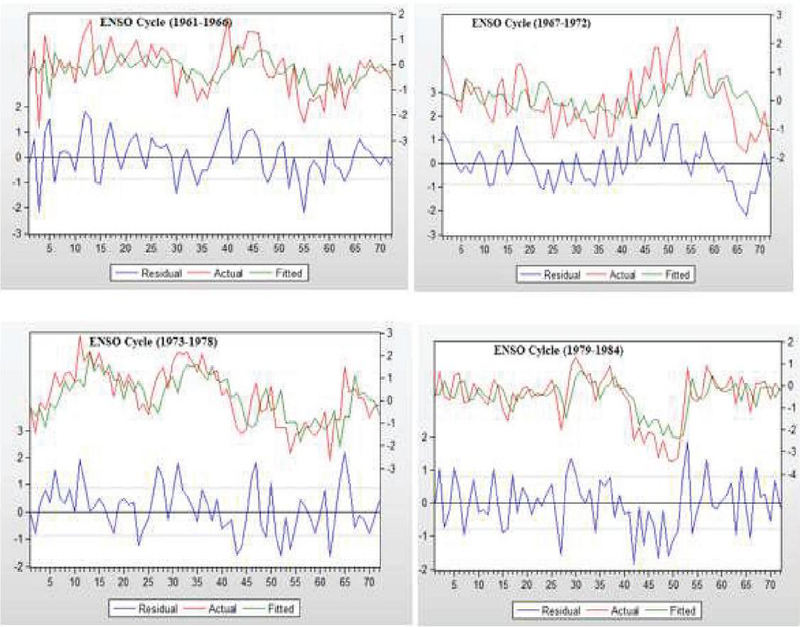
Figure 1 Actual values, fitted values and Residual value of AR (R) – GARCH (1, 1) Model of ENSO Cycles.
Figure 1 describe that Actual values, fitted values and Residue graph of ENSO Cycles which are shows that Actual values and fitted values have same behavior that shows the given dataset is good predictable. Actual values, Fitted values and Residue graph of AR (2) – GARCH (1, 1) Model of ENSO Cycle (1961–1966). All three parameters move along with slight deviation which exhibit efficacy of such model. Actual values, Fitted values and Residue graph of AR (5) – GARCH (2, 1) Model of ENSO Cycle (1967–1972). It shows tendency of appropriateness as the values of the three change persistently. Actual values, Fitted values and Residue graph of AR (2) – GARCH (1, 1) Model of ENSO cycle (1973–1978). In this cycle the fitted values show some dissimilarity with actual and residues. For Actual values, Fitted values and Residue graph of AR (1) – GARCH (1, 1) Model of ENSO cycle (1979–1984). For this cycle there is minimum regression between fitted values and actual values.
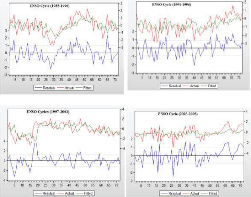
Figure 2 Actual values, fitted values and Residual value of AR (R) – GARCH (1, 1) Model of ENSO Cycles.
Figure 2 shows that for Actual values, Fitted values and Residue graph of AR (3) – GARCH (1, 1) Model of ENSO cycle (1985–1990). There is a slight contrast between actual and residual values though coincide as well on some levels. For Actual values, Fitted values and Residue graph of AR (3) – GARCH (2, 1) Model of ENSO cycle (1991–1996). Actual values match with error terms involved in each calculation while it has minor uneven distribution with fitted values. For Actual values, Fitted values and Residue graph of AR (1) – GARCH (1, 2) Model of ENSO cycle (1997–2002). We can see similarities between Actual and Fitted values on most of the points with subsequent Residual error. For Actual values, Fitted values and Residue graph of AR (2) – GARCH (1, 1) Model of ENSO cycle (2003–2008). There are relative values of both actual and fitted values and some exact overlapping can also be observed.
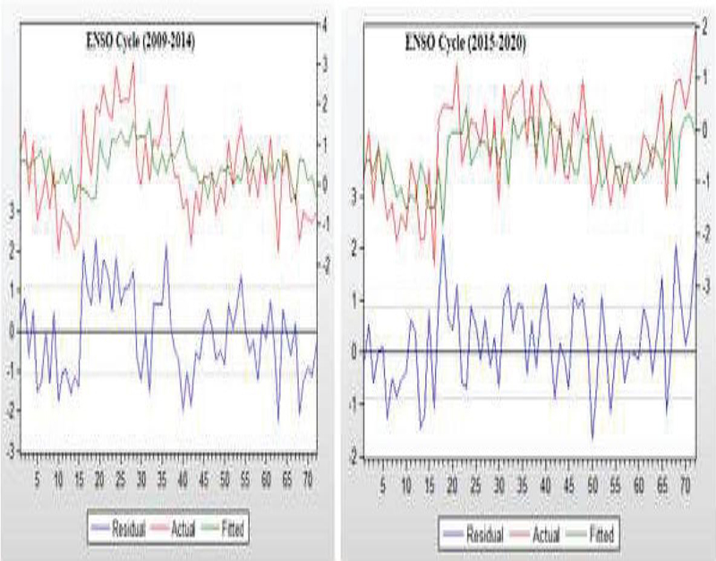
Figure 3 Actual values, fitted values and Residual value of AR (R) – GARCH (1, 1) Model of ENSO Cycles.
Figure 3 describe for Actual values, Fitted values and Residue graph of AR (4) – GARCH (1, 2) Model of ENSO cycle (2009–2014). The fitted values tend to lag behind actual value with equivalent fluctuation. The Actual values, Fitted values and Residue graph of AR (2) – GARCH (1, 2) Model of ENSO cycle (2015–2020). Here fitted values turn round between limitations of actual values and do not exceed on any of the point.
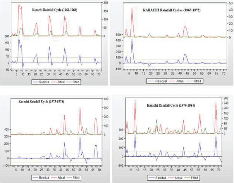
Figure 4 Actual values, fitted values and Residual value of AR (R) – GARCH (1, 1) Model of Rainfall Karachi Cycles.
Figure 4 describe that Actual values, fitted values and Residue graph of AR (R) – GARCH (1, 1) Model of Rainfall Karachi Cycles which show that Actual values and fitted values have same behavior that shows the given dataset is good predictable. Actual values, Fitted values and Residue graph of AR (1) – GARCH (1, 1) Model of Rainfall Cycle (1961–1966). All of three regression parameters follow almost constant distribution. Actual values, Fitted values and Residue graph of AR (12) – GARCH (1, 2) Model of Rainfall Cycle (1967–1972). Here the fitted values follow the actual trends with considerable difference on few iterations. Actual values, Fitted values and Residue graph of AR (15) – GARCH (1, 1) Model of Rainfall Cycle (1973–1978). In this cycle fitted values behave inactively in Rainfall months with approximately followed residues. Actual values, Fitted values and Residue graph of AR (16) – GARCH (1, 1) Model of Rainfall Cycle (1979–1984). Fitted values vary similarly along actual values with low equivocation.
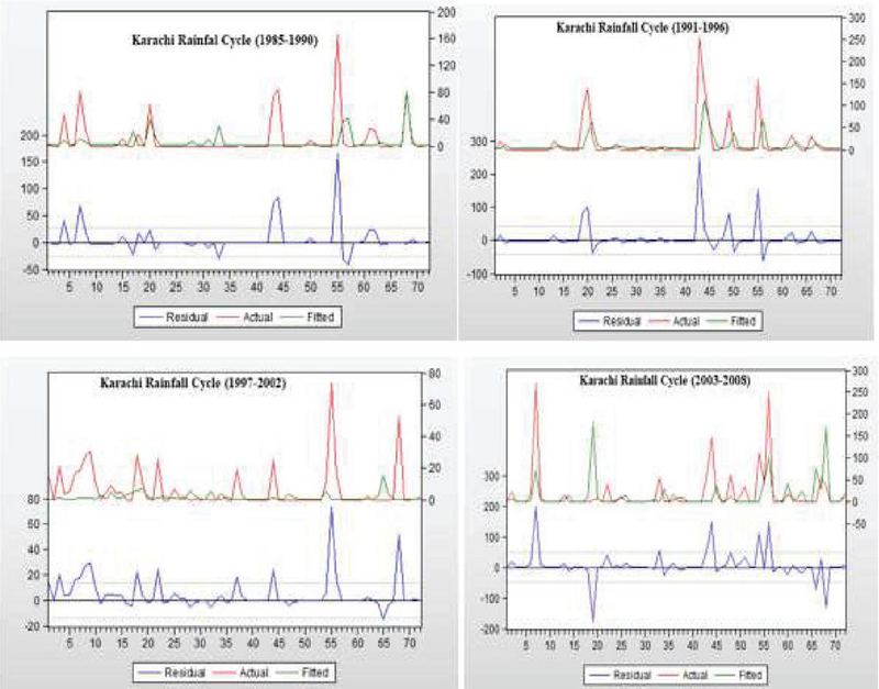
Figure 5 Actual values, fitted values and Residual value of AR (R) – GARCH (1, 1) Model of Rainfall Karachi Cycles.
Figure 5 shows that the Actual values, Fitted values and Residue graph of AR (13) – GARCH (1, 2) Model of Rainfall Cycle (1985–1990). Upon changing parameters fitted values do not follow actual values except on few stages. Actual values, Fitted values and Residue graph of AR (1) – GARCH (1, 1) Model of Rainfall Cycle (1991–1996). By altering parameters, the fitted values diverge from the actual values, with only a few terms exhibiting alignment. Actual values, Fitted values and Residue graph of AR (10) – GARCH (1, 2) Model of Rainfall Cycle (1997–2002). Fitted values occur with low randomness so it can be termed as poor fitness of the Model. Actual values, Fitted values and Residue graph of AR (12) – GARCH (1, 2) Model of Rainfall Cycle (2003–2008). This cycle’s distributions are apparently compelling on same points thus shows good relevance between the values.
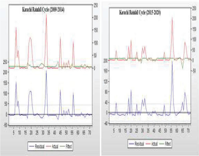
Figure 6 Actual values, fitted values and Residual value of AR (R) – GARCH (1, 1) Model of Rainfall Karachi Cycles.
Figure 6 describe that the Actual values, Fitted values and Residue graph of AR (10) – GARCH (1, 1) Model of Rainfall Cycle (2009–2014). The fitted values consistently change along the actual values, demonstrating harsh ambiguity. Actual values, Fitted values and Residue graph of AR (9) – GARCH (1, 1) Model of Rainfall Cycle (2015–2020). Less relevance can be seen in actual and found values, where residue terms move just along.
5.2 GARCH (P, Q) Process
Regression can actually be fitting a function in datasets and to make the function workable, it needs analysis of regression to generate the relationship of function to conclude the system of model bearing good outcomes. This model is useful when the variance is not constant for error terms. Heteroskedasticity shows the variation of irregular pattern in statistical model. GARCH models are specifically used for climatic modeling to notice log returns (Zheng. Et.al 2018). The non-stationary situation of the conditional variance shows results of AR-GARCH and according to criterions of either AIC or BIC the appropriate model might be AR (1) – GARCH (1, 1). The differences of samples will be the mean centered process, the white noise with a type of autoregression process has conditional heteroskedasticity to seek for feasible model, and the parameters p & q are actually order of noise. The research is suggesting that ENSO/Rainfall forecasts which may have non-stationary conditional variance, and the results of AR-GARCH indicate the non-stationary persistence. The datasets alike Rainfall and ENSO which is highly unpredictable hence GARCH model select with autoregression which is Heteroskedasticity defined an uncommon sample of error term variability or variance in a statistical form (Helmut Pruscha 2016). This paper analyses classified autoregression period along with white noise and conditional heteroskedasticity variance.
Table 5 Diagnostic Test of GARCH (P, Q) for ENSO Cycles (1st to 10th)
| Cycles | GARCH | R | ADJ R | SE-Reg. | Log Likel. | AIC. | SC. | HQC. | DW. |
| 1961–1966 | (1,2) | 0.87631 | 0.031785 | 0.935270 | -87.25631 | 2.5626 | 2.72077 | 2.625 | 1.121 |
| 1967–1972 | (1,1) | 0.7876 | 0.000796 | 0.998029 | -100.2851 | 2.8412 | 2.90449 | 2.866 | 0.611 |
| 1973–1978 | (3,1) | 0.9865 | 0.010225 | 1.228441 | -109.2778 | 3.2021 | 3.39188 | 3.277 | 0.501 |
| 1979–1984 | (1,1) | 0.8457 | 0.001700 | 1.088290 | -99.49280 | 2.8194 | 2.88248 | 2.844 | 0.597 |
| 1985–1990 | (1,1) | 0.9854 | 0.000008 | 1.099926 | -106.0780 | 3.0021 | 3.06540 | 3.027 | 0.715 |
| 1991–1996 | (1,1) | 0.7566 | 0.026105 | 1.000268 | -100.9962 | 2.8610 | 2.92424 | 2.886 | 0.907 |
| 1997–2002 | (1,1) | 0.76521 | 0.201814 | 1.385257 | -106.9385 | 3.1094 | 3.26750 | 3.172 | 0.455 |
| 2003–2008 | (1,1) | 0.76521 | 0.001595 | 0.998962 | -104.4412 | 2.9567 | 3.01994 | 2.981 | 1.296 |
| 2009–2014 | (1,1) | 0.84654 | 0.069884 | 1.186764 | -110.0817 | 3.0856 | 3.11722 | 3.098 | 0.796 |
| 2015–2020 | (1,1) | 0.96578 | 0.091745 | 0.949992 | -97.39816 | 2.7610 | 2.82430 | 2.786 | 1.102 |
Table 5 Accordingly, by way of combining those models autoregression and GARCH wherein AR (p) is applied to the time series variance at the same time as GARCH (p, q) technique used in time series. The selection of appropriate model technique depends on Durbin-Watson statistics test and by values we see strong autocorrelation in the dataset. Least-square estimation is also estimated for GARCH and it shows the diagnostic test which is conducted with same method; model fitness is checked by AIC, HQC and BIC; Information criteria. Lower values indicate better model fit. Likelihood Ratio test compares the likelihood of the estimated model against a simple model. It helps to determine if more complex GARCH model significantly improves the fit. All cycles show that best appropriate model is GARCH (1, 1) process apart from few iterations.
Table 6 The Evolution of Forecast of ENSO Cycles by GARCH (P, Q) model of cycle (1st to 10th)
| Cycles | GARCH | RMSE | MAE | MAPE | U-Test |
| 1961–1966 | (1,2) | 0.9287 | 0.7405 | 227.98 | 0.7497 |
| 1967–1972 | (1,1) | 0.9910 | 0.806 | 99.366 | 0.97388 |
| 1973–1978 | (3,1) | 1.21988 | 1.0312 | 101.234 | 0.8445 |
| 1979–1984 | (1,1) | 1.0807 | 0.7916 | 248.71 | 0.6418 |
| 1985–1990 | (1,1) | 1.0922 | 0.8743 | 115.6 | 0.8844 |
| 1991–1996 | (1,1) | 0.9932 | 0.8319 | 479.90 | 0.4650 |
| 1997–2002 | (1,1) | 1.3756 | 1.0682 | 133.49 | 0.8132 |
| 2003–2008 | (1,1) | 0.99200 | 0.78441 | 125.519 | 0.9120 |
| 2009–2014 | (1,1) | 1.1867 | 0.9498 | 100.00 | 1.0000 |
| 2015–2020 | (1,1) | 0.943372 | 0.79410 | 190.146 | 0.7235 |
Table 6 describe that the GARCH modeling is performed for climate volatility along with evaluation metrics (RMSE, MAE, MAPE) and a measure of inequality (Theil Index). MAE is often used when the emphasis is on the magnitude of errors, while MAPE is useful when the emphasis is on the percentage difference. Both climatic indices show less relation as values are deviating from zero. Thus GARCH (P, Q) model is proving to be rarely responsive for ENSO relation with other weather epochs.
Table 7 Diagnostic Test of GARCH (P, Q) for Rainfall Cycles (1st to 10th)
| Cycles | GARCH | R | ADJ R | SE-Reg. | Log Likel. | AIC. | SC. | HQC. | DW. |
| 1961–1966 | (2,1) | 0.8166 | -0.166651 | 47.00131 | -355.9897 | 10.027 | 10.1855 | 10.09 | 0.797 |
| 1967–1972 | (1,1) | 0.7079 | -0.079820 | 61.56519 | -369.9068 | 10.386 | 10.5127 | 10.43 | 1.371 |
| 1973–1978 | (1,1) | 0.8116 | -0.116326 | 56.02249 | -336.1849 | 9.4495 | 9.57598 | 9.499 | 1.403 |
| 1979–1984 | (1,1) | 0.9187 | -0.187475 | 53.28809 | -372.7670 | 10.465 | 10.5922 | 10.51 | 1.707 |
| 1985–1990 | (2,1) | 0.8042 | -0.042124 | 28.25733 | -332.6192 | 9.3783 | 9.53641 | 9.441 | 1.813 |
| 1991–1996 | (2,1) | 0.6978 | -0.069956 | 45.16401 | -347.5970 | 9.7943 | 9.9524 | 9.857 | 1.229 |
| 1997–2002 | (1,1) | 0.7268 | -0.068620 | 13.14148 | -270.8147 | 7.6337 | 7.76022 | 7.684 | 1.570 |
| 2003–2008 | (2,1) | 0.9123 | -0.123181 | 51.35833 | -353.1582 | 9.9488 | 10.106 | 10.01 | 1.652 |
| 2009–2014 | (1,1) | 0.7032 | -0.032828 | 42.49825 | -350.7331 | 9.8536 | 9.98017 | 9.904 | 1.428 |
| 2015–2020 | (2,1) | 0.8124 | -0.124066 | 34.56743 | -332.3598 | 9.3711 | 9.5292 | 9.434 | 1.226 |
Table 7 shows positive autocorrelation and standard error is regressed minimally in 7th cycle; further endorsed by log-likelihood function. However, on R-squared values shows that positive correlation. model fitness is checked by AIC, HQC and BIC; Information criteria. Lower values indicate better model fit. Likelihood Ratio test compares the likelihood of the estimated model against a simple model. All cycles show that best appropriate model is GARCH (P, Q) process.
Table 8 The Evolution of Forecast of Karachi Rainfall Cycles by GARCH (P, Q) model (1st to 10th)
| Cycles | GARCH (p, q) | RMSE | MAE | MAPE | U-Test |
| 1961–1966 | (2,1) | 46.67 | 18.518 | 23.228 | 0.9832 |
| 1967–1972 | (1,1) | 61.136 | 19.269 | 37.543 | 0.9567 |
| 1973–1978 | (1,1) | 55.632 | 21.415 | 112.01 | 0.9351 |
| 1979–1984 | (1,1) | 52.916 | 21.025 | 50.553 | 0.9965 |
| 1985–1990 | (2,1) | 28.060 | 12.42 | 103.62 | 0.8308 |
| 1991–1996 | (2,1) | 44.849 | 17.685 | 85.920 | 0.8771 |
| 1997–2002 | (1,1) | 13.049 | 6.917 | 110.15 | 0.7662 |
| 2003–2008 | (2,1) | 51.000 | 19.472 | 58.658 | 0.9442 |
| 2009–2014 | (1,1) | 42.202 | 22.265 | 225.12 | 0.7575 |
| 2015–2020 | (2,1) | 34.326 | 15.04 | 51.693 | 0.8923 |
Table 8 indicates a slight correlation between the better Thiel’s U outcome and the anticipated evolution of rainfall Karachi cycles. It should be noted that, using ENSO’s guidance, we applied Thiel’s-U by contrasting the predicted and actual observed rainfall values. Both the size and direction of change mistakes are retained in the calculation. Additional popular measures are MAE, RMSE, and MAPE. The objectives of the forecasting endeavor and the unique properties of the data will determine which metric is used.
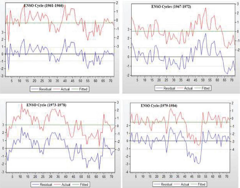
Figure 7 Actual values, fitted values and Residual value of GARCH (P, Q) Model of ENSO Cycles.
Figure 7 describe that Actual values, fitted values and Residue graph of GARCH (P, Q) technique of all ENSO cycles which show that Actual values and fitted values have same behavior that shows the given dataset is good predictable. The actual values, Fitted values and Residue graph of GARCH (1, 2) Model of ENSO Cycle (1961–1966). In this cycle the calculations have shown absolute La-Nina condition. It might be this Model’s weakness. The actual values and Fitted values and Residue graph of GARCH (1, 1) Model of ENSO Cycle (1967–1972). The model is indicating La-Nina condition. Actual values, Fitted values and Residue graph of GARCH (3, 1) Model of ENSO Cycle (1973–1978). Normal condition persisted by such model, which is termed as La-Nina. Actual values and Fitted values and Residue graph of GARCH (1, 1) Model of ENSO Cycle (1979–1984). No fluctuation shown by fitted values.
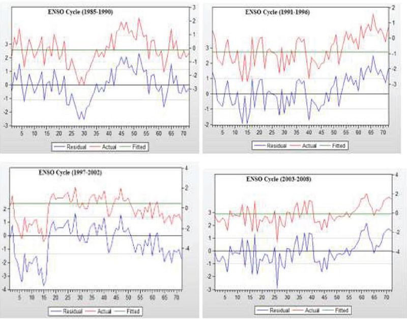
Figure 8 Actual values, fitted values and Residual value of GARCH (P, Q) Model of ENSO Cycles.
Figure 8 describe that the actual values and the fitted values and residue graph of GARCH (1, 1) Model of ENSO Cycle (1985–1990). Parameters of merely previous year could not confirm ENSO’s existence. Actual values, Fitted values and Residue graph of GARCH (1, 1) Model of ENSO Cycle (1991–1996). No distribution at all for fitted values. Actual values, Fitted values and Residue graph of GARCH (1, 1) Model of ENSO Cycle (1997–2002). ENSO cycles extend by two to seven years; hence limited observations cannot help find intensity of the phenomena. Actual values, Fitted values and Residue graph of GARCH (1, 1) Model of ENSO Cycle (2003–2008). Same results persist.
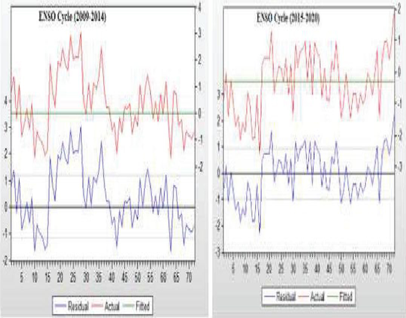
Figure 9 Actual values, fitted values and Residual value of GARCH (P, Q) Model of ENSO Cycles.
Figure 9 describe that the Actual values, fitted values and Residue graph of GARCH (1, 1) Model of ENSO Cycle (2009–2014) are same results persist. Actual values, Fitted values and Residue graph of GARCH (1, 1) Model of ENSO Cycle (2015–2020). This model performs monotonously.
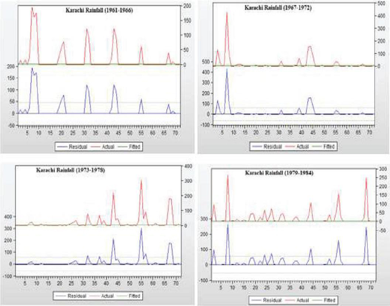
Figure 10 Actual values, fitted values and Residual value of GARCH (P, Q) Model of Rainfall Karachi Cycles.
Figures 10 describe that Actual values, fitted values and Residue graph of GARCH (P, Q) Model of Rainfall Karachi Cycles which show that Actual values and fitted values have same behavior that shows the given dataset is good predictable. Actual values, Fitted values and Residue graph of GARCH (2, 1) Model of Rainfall Cycle (1961–1966). Fitted values resulted in no rain at all. Actual values, Fitted values and Residue graph of GARCH (1, 1) Model of Rainfall Cycle (1967–1972). Same situation persists. Actual values, Fitted values and Residue graph of GARCH (1, 1) Model of Rainfall Cycle (1973–1978). This model has identical behavior. Actual values, Fitted values and Residue graph of GARCH (1, 1) Model of Rainfall Cycle (1979–1984).
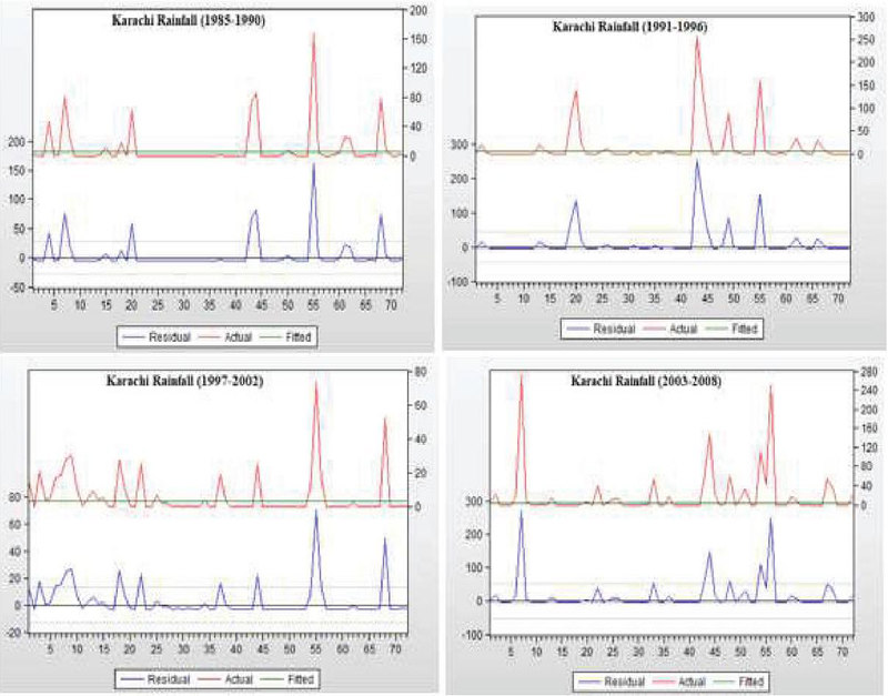
Figure 11 Actual values, fitted values and Residual value of GARCH (P, Q) Model of Rainfall Karachi Cycles.
Figure 11 describe the Actual values, fitted values and Residue graph of GARCH (2, 1) Model of Rainfall Cycle (1985–1990). Actual values, Fitted values and Residue graph of GARCH (2, 1) Model of Rainfall Cycle (1991–1996). Actual values, Fitted values and Residue graph of GARCH (1, 1) Model of Rainfall Cycle (1997–2002). Actual values, fitted values and Residue graph of GARCH (2, 1) Model of Rainfall Cycle (2003–2008) are is persists.
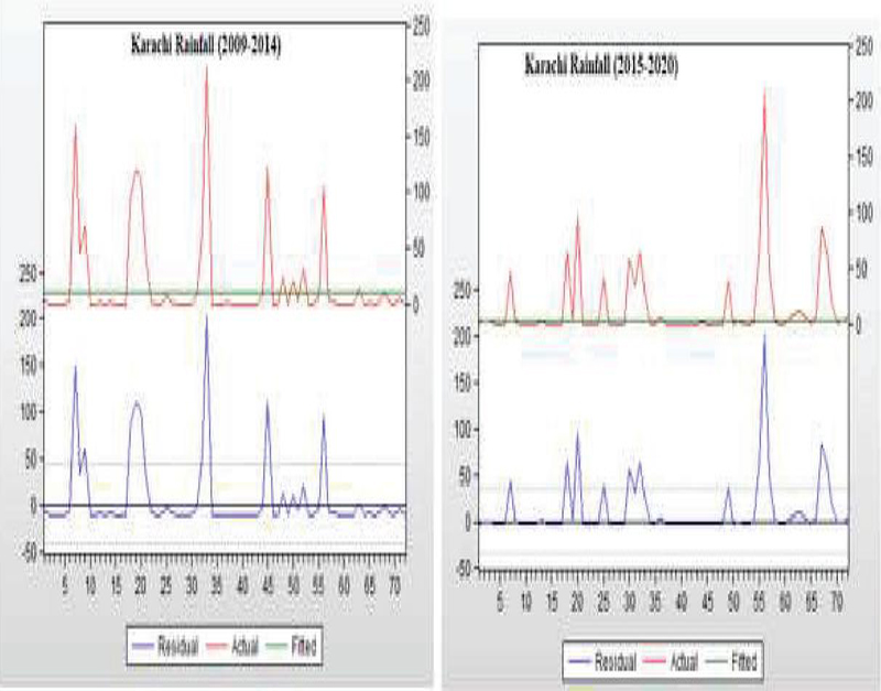
Figure 12 Actual values, fitted values and Residual value of GARCH (P, Q) Model of Rainfall Karachi Cycles.
Figure 12 described that the Actual values, Fitted values and Residue graph of GARCH (2, 1) Model of Rainfall Cycle (2009–2014). Actual values, Fitted values and Residue graph of GARCH (2, 1) Model of Rainfall Cycle (2015–2020).
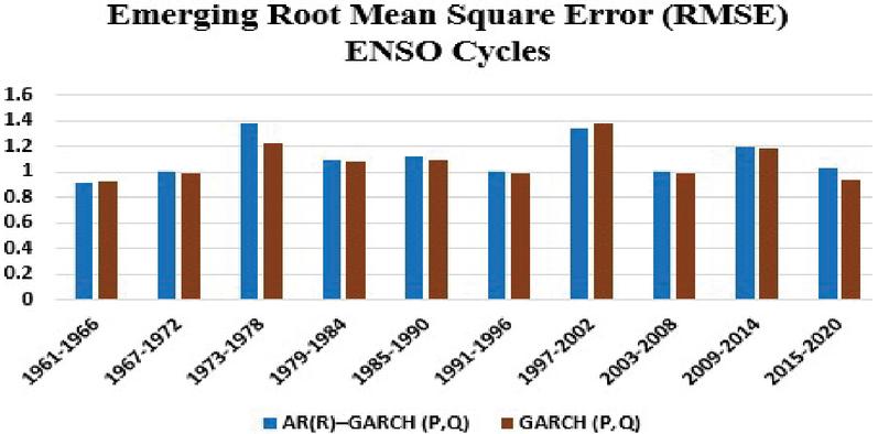
Figure 13 Emerging Root Mean Square Error (RMSE) of GARCH (P, Q) and AR (R)-GARCH (P, Q) model for ENSO Cycles (1st to 10th).
Figure 13 describe that the comparison of Emerging Root Mean Square Error (RMSE) of AR (R)-GRACH (P, Q) and GRACH (P, Q) model of ENSO Cycles (1st-10th). This figure shows that GRACH (P, Q) Model performed better than its combined other model.
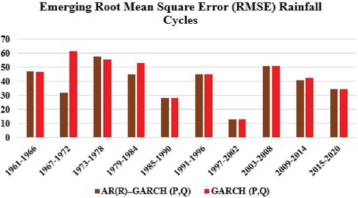
Figure 14 Emerging Root Mean Square Error (RMSE) of GARCH (P, Q) and AR (R)-GARCH (P, Q) Model for Karachi Rainfall Cycles (1st to 10th).
Figure 14 shows that the comparison of Emerging Root Mean Square Error (RMSE) of AR (R)-GRACH (P, Q) and GRACH (P, Q) model of Rainfall Cycles (1st-10th). This figure describes that GRACH (P, Q) Model performed better than its combined form with other model.
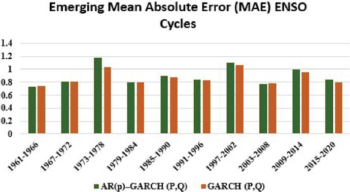
Figure 15 Emerging Mean Absolute Error (MAE) of GARCH (P, Q) and AR (R)-GARCH (P, Q) Model for ENSO Cycles (1st to 10th).
Figure 15 describe that the comparison of Emerging Mean Absolute Error (MAE) of AR (R)-GRACH (P, Q) and GRACH (P, Q) model of ENSO Cycles (1st-10th). This figure clearly shows that GRACH (P, Q) Model performed better than its combined form with other model.
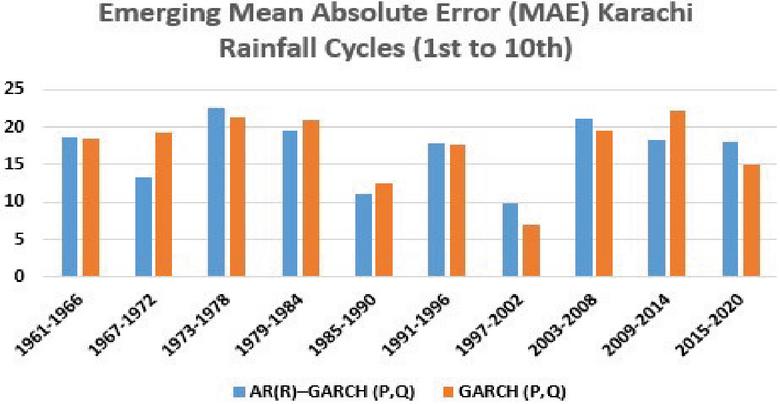
Figure 16 Emerging Mean Absolute Error (MAE) of GARCH (P, Q) and AR (R)-GARCH (P, Q) Model for Rainfall Cycles (1st to 10th).
Figure 16 explain the Emerging Mean Absolute Error (MAE) of GARCH (P, Q) and AR (R)-GARCH (P, Q) Model for Rainfall Cycles (1st to 10th). Majority cycles shows that the GARCH (P, Q) model performance is better than others.
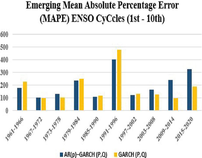
Figure 17 Emerging Mean Absolute Percentage Error (MAPE) of GARCH (P, Q) and AR (R)-GARCH (P, Q) Model for ENSO Cycles (1st to 10th).
Figure 17 describe that the comparison of Emerging Mean Absolute Percentage Error (MAPE) of AR (R)-GRACH (P, Q) and GRACH (P, Q) model of ENSO Cycles (1st-10th). This figure clearly shows that GRACH (P, Q) Model performed better than its combined form with other model.
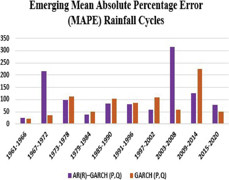
Figure 18 Emerging Mean Absolute Percentage Error (MAPE) of GARCH (P, Q) and AR (R)-GARCH (P, Q) Model for Rainfall Cycles (1st to 10th).
Figure 18 explain the Emerging Mean Absolute Percentage Error (MAPE) of GARCH (P, Q) and AR (R)-GARCH (P, Q) Model for Rainfall Cycles (1st to 10th). Majority cycles shows that the GARCH (P, Q) model performance is better than others.
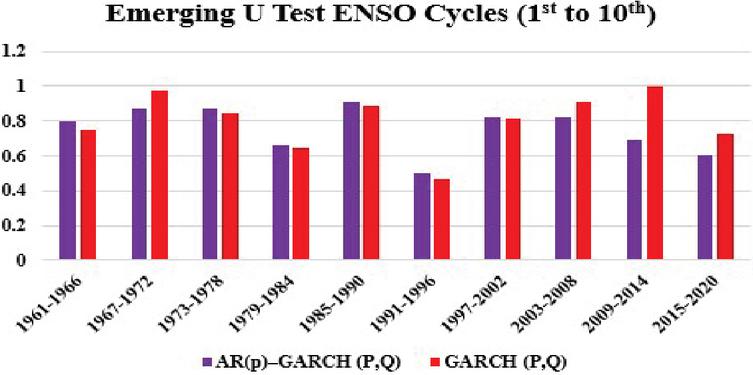
Figure 19 Emerging U Test of GARCH (P, Q) and AR (R)-GARCH (P, Q) Model for ENSO Cycles (1st to 10th).
Figure 19 describe that the comparison of Emerging U Test of AR (R)-GRACH (P, Q) and GRACH (P, Q) model of ENSO Cycles (1st-10th). This figure clearly shows that GRACH (P, Q) Model performed better than its combined form with other model.
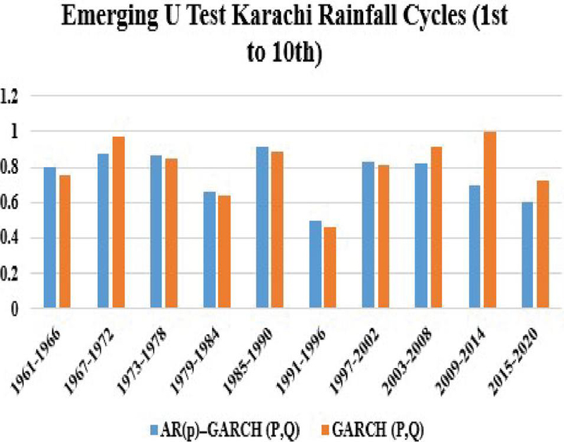
Figure 20 Emerging U Test of GARCH (P, Q) and AR (R)-GARCH (P, Q) Model for Rainfall Cycles (1st to 10th).
Figure 20 describe that the comparison of Emerging U Test of AR (R)-GRACH (P, Q) and GRACH (P, Q) model of Rainfall Cycles (1st-10th). This figure clearly shows that GRACH (P, Q) Model performed better than its combined form with other model.
6 Conclusion
This study addressed climatological condition due to ENSO and Rainfall, both are studied with their datasets and conclusively their comparative study is focused; that’s how they deal with each other especially, ENSO effecting Rainfall on region of Karachi. This phenomenon may arise due to the existence of alternative specifications, which are differentiating its nature by the time. The AR (R)-GARCH (P, Q) process time series model is suitable if the time variable renders an autoregression which is considered for the error variance. There is a methodological technique between ENSO and Rainfall cycles dataset for a casual determination with practically observed forecasts in limited time series dataset, which has resulted for the necessity of inferred study of forecasting accurately and choosing any method for forecasting, which behave simply as well as effectively. The practical methods based on ENSO for precipitation noticed, are higher from Oct Dec, also the prediction of rainfall is normal in the period; Jan to Sept, the combination of ENSO impact on the period Jan till March and July to Aug by approaching to excessive implication for many regions, in case of low stream flow from Arabian Sea while there is an active El-Nino episodes going on. In these Months; from July to August Karachi receives much Rainfall annually. Sometimes the spontaneous climatic vibes confirm the schematic representation of sea surface condition of Indian Ocean and land surface of the specific region, while performing modeling about ENSO. El-Niño usually reduces rainfalls, droughts, and disturbs weather patterns. However, the results of it on a specific location like Karachi depends on various other factors as well, including the severity and duration of the ENSO episodes, along other regional climatological factors. In August, 2020, Karachi had had highest Rainfall of 366.8 mm (PMD; Karachi extremes, 2020), which is said to be latest weather anomaly driven by ENSO to the city.
The generalized autoregressive heteroskedasticity, GARCH is an important process of approaching volatility by an estimation of ENSO/Rainfall dataset. In model of GARCH (P, Q) current volatility is affected by its previous record as well as by its previous volatility variation of other time series. We fixed GARCH model with time series preceding or subsequent to the ten cycles, which assess an alteration in the heteroskedastic characteristics of ENSO Index. GARCH model for the ENSO and Rainfall cycles are numerically essential for both periods. It will make us better to infer the relation of both time series, i.e., significantly ENSO/Rainfall and drought condition. Otherwise, it can indicate a minor impact of ENSO on Rainfall with respect to randomly correlated coefficient. Conclusively, the bivariate GARCH models have shown stronger conditional correlation of ENSO on Rainfall as compared to unconditional correlation. It’s important to note that the impacts of ENSO events on local weather patterns are complex and can vary from one event to another. Additionally, regional climate influences, local geography, and other atmospheric patterns can also play a significant role in determining how ENSO affects a specific area like Karachi.
Acknowledgments
The authors are also thankful to the World Data Centre (WDC) and National Oceanic and Atmospheric Administration (NOAA) for providing the ENSO data and Pakistan Metrological department provide Karachi Rainfall Data.
References
[1] Johnson, N. C., Collins, D. C., Feldstein, S. B., L’Heureux, M. L., and Riddle, E. E. (2014). Skillful wintertime North American temperature forecasts out to 4 weeks based on the state of ENSO and the MJO. Weather and Forecasting 29(1), 23–38.
[2] Ropelewski, C. F., and Halpert, M. S. (1987). Global and regional scale precipitation patterns associated with the El Niño/Southern Oscillation. Monthly weather review. 115(8), 1606–1626.
[3] Shabbar, A., and Khandekar, M. (1996). The impact of el Nino-Southern oscillation on the temperature field over Canada: Research note. Atmosphere-Ocean. 34(2), 401–416.
[4] Timmermann, A., Oberhuber, J., Bacher, A., Esch, M., Latif, M., and Roeckner, E. (1999). Increased El Niño frequency in a climate model forced by future greenhouse warming. Nature. 398(6729), 694–697.
[5] Wang, B., Wu, R., and Fu, X. (2000). Pacific–East Asian teleconnection: how does ENSO affect East Asian climate?. Journal of climate. 13(9), 1517–1536.
[6] Boucharel, J., Dewitte, B., du Penhoat, Y., Garel, B., Yeh, S. W., and Kug, J. S. (2011). ENSO nonlinearity in a warming climate. Climate Dynamics. 37, 2045–2065.
[7] Phillips, O. L., Aragão, L. E., Lewis, S. L., Fisher, J. B., Lloyd, J., López-González, G., … and Torres-Lezama, A. (2009). Drought sensitivity of the Amazon rainforest. Science. 323(5919), 1344–1347.
[8] Kumar, K. K., Rajagopalan, B., and Cane, M. A. (1999). On the weakening relationship between the Indian monsoon and ENSO. Science. 284(5423), 2156–2159.
[9] Afaq, F., Syed, D. N., Malik, A., Hadi, N., Sarfaraz, S., Kweon, M. H., … and Mukhtar, H. (2007). Delphinidin, an anthocyanidin in pigmented fruits and vegetables, protects human HaCaT keratinocytes and mouse skin against UVB-mediated oxidative stress and apoptosis. Journal of Investigative Dermatology. 127(1), 222–232.
[10] Liu, H., and Shi, J. (2013). Applying ARMA–GARCH approaches to forecasting short-term electricity prices. Energy Economics. 37, 152–166.
[11] Kim, T., Shin, J. Y., Kim, H., Kim, S., and Heo, J. H. (2019). The use of large-scale climate indices in monthly reservoir inflow forecasting and its application on time series and artificial intelligence models. Water. 11(2), 374.
[12] Adhikari. (2014) Adhikari R. 2013: Introduction of time series modeling & forecasting, University of Cornell.
[13] Ghani, I. M., and Rahim, H. A. Modeling and forecasting of volatility using arma-garch: Case study on malaysia natural rubber prices. In IOP Conference Series: Materials Science and Engineering. June 2019.
[14] Hyndman, R. J., and Koehler, A. B. (2006). Another look at measures of forecast accuracy. International journal of forecasting. 22(4), 679–688.
[15] Tsay, R. S. (2000). Time series and forecasting: Brief history and future research. Journal of the American Statistical Association. 95(450), 638–643.
[16] Bollerslev, T. (1986). Generalized autoregressive conditional heteroskedasticity. Journal of econometrics. 31(3), 307–327.
[17] Jalal Uddin Jamali, A. R. M., Asadul Alam, M., and Aziz, A. (2021). Statistical Analysis of Various Optimal Latin Hypercube Designs. Data Science and SDGs: Challenges, Opportunities and Realities. 155–163.
[18] Zaffar, A., Abbas, S., and Ansari, M. R. K. (2022). Model estimation and prediction of sunspots cycles through AR-GARCH models. Indian Journal of Physics. 96(7), 1895–1903.
[19] Pal, S., Islam, A. R. M. T., Patwary, M. A., and Alam, G. M. 2021. Modeling household socio-economic vulnerability to natural disaster in teesta basin, Bangladesh. Climate Vulnerability and Resilience in the Global South: Human Adaptations for Sustainable Futures. 103–129.
[20] Zheng, B., Tong, D., Li, M., Liu, F., Hong, C., Geng, G., … and Zhang, Q. 2018. Trends in China’s anthropogenic emissions since 2010 as the consequence of clean air actions. Atmospheric Chemistry and Physics. 18(19), 14095–14111.
Biographies

Asma Zaffar received the bachelor’s degree, M. Phil and Ph.D. entitled Morphology and image analysis of some solar photospheric phenomena in Mathematics from University of Karachi. Currently serve as an Associate Professor and Chairperson of the department of Mathematics and Sciences, Sir Syed University of Engineering and Technology. She has been HEC approved supervisor from 2019 and published numerous research articles in different national and international reputed journals. Her research area is Time series analysis, Astrophysics, Data Analysis, Homological Algebra and Climate Change.

Rizwan Khan received the bachelor’s degree in Mathematics from University of Karachi and received Master entitle Impact of El-Nino Southern Oscillation (ENSO) on the Rainfall of Karachi Region from the department of Mathematics and Sciences, Sir Syed University of Engineering and Technology in 2023.

Nimra Malik received the bachelor’s degree in civil engineering from NED University in 2014, the master’s degree in engineering management from institute of business management. Currently working as Business Development Manager at National Center of GIS and Space Applications (NCGSA), Institute of Space Technology (IST) Islamabad, Pakistan.

Muhammad Aamir received an MS degree in Electronic Engineering (with specialization in Telecommunication) in 2002 and a BS in Electronic Engineering in 1998 from Sir Syed University of Engineering and Technology Karachi. He accomplished his PhD in Electronic Engineering from Mehran University of Engineering & Technology Jamshoro in December 2014. During his PhD studies, he accomplished major part of his research work at the University of Malaga Spain under Erasmus Mundus Scholarship. He has authored and co-authored around 50 research papers and book chapters published in various journals, books and conferences of international repute including more than 15 papers with co-authorship of Professors from Mehran University of Engineering & Technology. He is a life member of Pakistan Engineering Council and senior member of IEEE and currently serving as chair of IEEE Communication Society for Karachi Chapter. He was awarded with a grant by the Ministry of Education Spain to teach at the University of Malaga which he successfully availed in May 2012. He had also served as Member of two separate National Curriculum Revision Committees constituted by Higher Education Commission (HEC) for revision of Electronic Engineering Curriculum and Telecommunication Engineering Curriculum at the National Level. He is currently associated with Sir Syed University of Engineering & Technology as Professor and Dean in the Faculty of Electrical & Computer Engineering. Additionally, he is also Editor-in-Chief of Sir Syed University Research Journal of Engineering & Technology (HEC Recognized Journal) which is published bi-annually. He has been included in the Stanford University’s top 2% global scientists list. The US-based Stanford University released a list in October 2020 that represents the top 2% of the most-cited scientists in multiple disciplines. The list comprises around 160,000 persons from all over the world while only 243 Pakistani were included in the list so it is a unique honor that an alumni of Sir Syed University of Engineering & Technology is recognized at International level within top 2% global scientists in multidisciplinary research.

Vali Uddin Presently serving as Vice Chancellor, Sir Syed University of Engineering & Technology, Karachi. Vali Uddin earlier served at Hamdard University, Karachi, as Professor, (July 2011 – June 2019), Acting Vice Chancellor (from October 24 till October 31, 2013, and July 22, 2014 till August 29, 2014), Dean, Faculty of Engineering Sciences and Technology (July 2013 – May 2019), Registrar (April 2017 till October 2018), Acting Registrar, (August 2012 till August 2015) and, Director, Hamdard Institute of Information Technology, (July 2011 – July 2013). Vali Uddin earned his Ph.D. Electrical Engineering from Boston University, MA, USA.
Earlier, he did his BE (Electronics) from NED University, Karachi with First Class First Position and went on to do his MS Electrical Engineering from Boston University, Boston, MA. He was Conference Chairman of First and Second IEEE International Conference on Computer Control and Communication at PNEC-NUST, Karachi on 12–13 November 2007 and 17-18 February, 2009 respectively and Conference General Chair of 21st IEEE International Multi-topic Conference, Hamdard University Karachi held on November 01 – 02, 2018. He initiated BE (Electronics), BE (Telecommunication), MS (Computer Science), MS (Engineering), PhD (Computer Science) and PhD (Engineering) degree programs at Iqra University, Karachi as a Dean, Faculty of Engineering, Sciences and Technology. He initiated BE (Electrical) and BE (Mechanical) degree programs at Hamdard University as Dean, Faculty of Engineering, Sciences and Technology. He has been a key member of a team as Registrar who brought Financial turnaround of Hamdard University in less than two years. He has been a key member of a team member who developed and expanded MS and PhD programs at PNEC-NUST.

Muhammad Asif is currently working as a Professor and Dean of Computing and Applied Sciences, Sir Syed University of Engineering and Technology. He has Director Quality Enhancement Cell at Ziauddin University, Karachi, Pakistan. He is also the Principal Investigator of Data Acquisition, Processing and Predictive Laboratory (DAPPA), National Center in Big Data and Cloud Computing. In his lab, he is working on vehicle and traffic flow modeling and monitoring and environmental data collection to monitor environmental degradation and climate change using smart technologies with the blend of artificial intelligence. Dr. Muhammad Asif received B.S. degree in Biomedical Engineering from the Sir Syed University of Engineering and Technology, Karachi, Pakistan in 2002, and M.S. degree in Electrical Engineering from the Universiti Sains Malaysia (USM) Malaysia, in 2007. In USM, he worked with USM Robotics Research Group (URRG) on various underwater robotics and vision systems. In 2015, we received his Ph.D. in Electrical Engineering from NUST. He organized and participated in various robotics competition on national and international levels like ROBOCON, ROBOCOM, NERC, etc. He has more than 50 research publications in international and national journals and conferences.
Journal of Mobile Multimedia, Vol. 20_6, 1251–1288.
doi: 10.13052/jmm1550-4646.2064
© 2025 River Publishers