Forecasting Karachi’s Air Temperature Variation: Leveraging Mobile and Multimedia Dataset for Global Warming Insights
Asma Zaffar1,*, Shakil Ahmed2, Aysha Rafique3, Muhammad Imran4, Muhammad Amir5 and Vali Uddin6
1Department of Mathematics and Sciences, Sir Syed University of Engineering & Technology, Karachi, Pakistan
2Department of Computer Engineering, Sir Syed University of Engineering & Technology, Karachi, Pakistan
3Department of Telecommunication Engineering, Sir Syed University of Engineering & Technology, Pakistan
4Department of Civil Engineering, Sir Syed University of Engineering & Technology, Karachi, Pakistan
5Professor and Dean Computer and Electrical Engineering, Sir Syed University of Engineering & Technology, Karachi, Pakistan
6Professor and Vice Chancellor, Sir Syed University of Engineering & Technology, Karachi, Pakistan
E-mail: aszafar@ssuet.edu.pk; shakilab@ssuet.edu.pk; arafique@ssuet.edu.pk; mimran@ssuet.edu.pk; maamir@ssuet.edu.pk; drvali@ssuet.edu.pk
*Corresponding Author
Received 31 March 2024; Accepted 02 December 2024
Abstract
In Karachi, the transport and building industries have a major impact on carbon dioxide (CO) emissions and greenhouse gas emissions. This study is innovative in that it examines how air temperature changes over time and forecasts the maximum and minimum temperatures in Karachi. Specifically, it looks at 60 years’ worth of mean monthly maximum and minimum air temperatures in Karachi, spanning from (1961 to 2020) dataset classes. The monthly average air temperature in Karachi, both at its minimum and maximum, remains constant. Using dataset from the Pakistan Metrological Department (PMD) and, the ARMA (p, q) model technique was used to assess forecasting and modelling the behavior of the maximum and minimum air temperatures in Karachi. The least values Akaike information criterion (AIC), the Bayesian Schwarz information criterion (SIC), and the Hannan Quinn information criterion (HIC) are used to describe how adequate the model is. Additionally, the Durbin-Watson (DW) test is used. The average monthly maximum and minimum air temperature in Karachi are strongly correlated, as indicated by DW values (2). The lowest and maximum monthly average air temperatures in Karachi are predicted using diagnostic checking techniques such as Root Mean Squared Error (RMSE), Mean Absolute Error (MAE), Mean Absolute Percentage Error (MAPE), and Theil’s U-Statistics. The results indicate that there is a strong correlation between the air temperature and previously measured values, with Theil’s U-Statistics values for each month lying close to zero. This study is a great resource for observing how air temperature affects global warming. This study also highlights the the innovative aspect of utilizing vast datasets, possibly including those from mobile and multimedia sources, to address a critical environmental issue. It also emphasizes the predictive modelling aspect of your study, which is central to understanding and mitigating global warming effects.
Keywords: ARMA (p, q) model, air temperature, root mean square error, skewness, kurtosis.
1 Introduction
Global warming threatens our environment and human health. It also causes high temperatures, rising sea levels, droughts, and floods. There are a variety of features that contribute but the work of transportation and travel during the construction process contributes to the high GHG in the big city of Karachi [1]. The United Nations (UN) Office for Disaster Risk Reduction (UNDRR) between 2000 and 2019, heatwave accounted for 13% of all catastrophic deaths (91pc) worldwide. In addition, United Nations (UN) experts have warned Karachi to prepare for extraordinary temperatures as global temperatures rise by 1.1C and will continue to cause such disasters [2]. Historically, rising temperatures could have a direct impact on agriculture, the sea, and the prevalence of extreme weather. In the last few years especially from 2015 to 2020 the city of Karachi has experienced some very bad weather. Usually, May to June should be the hottest months before the onset of heavy rains in Karachi. Rays of solar radiation in the heat of the Day rise to 40 to 42C in parts of Sindh, including Karachi. According to the German clock, the German think tank in its current global climate risk report ranked Pakistan 05th in the list of the top 10 countries most affected by climate change [3] (https://reliefweb.int/report/pakistan/impact-climate-change-karachi-may-be-one-pakistan-s-biggest-threats. 2021). Karachi may be one of the most affected cities in Pakistan due to climate change. This large city cannot withstand the effects of global warming. There are several factors that contribute to global warming and CO emissions. However, construction work accounts for about 39% of all carbon emissions in the world (https://www.worldgbc.org/news-media/WorldGBC-embodied-carbon-report-published (2021). with the building performance of the building as a necessary accounting strength of about 28%. While 11% CO is emitted from the construction process, the logistics / production process, the life process and the demolition process.
In the middle of the airflow process it emits high temperatures and particles that increase global warming. Similarly, land transport does the same, releasing gases such as hydrocarbon, carbon dioxide, sulfur oxides, nitrogen, and black carbon etc. into the environment causing higher temperatures. CO is the only emissions from the construction and manufacturing industry with a total percentage of petrol consumption in Pakistan at 23.84 per cent from 2014 which was significantly higher than 43 years. Concrete, on the other hand, is the most common building material in Pakistan, known as the largest CO emitters that produce hazardous waste to the environment during processes related to its production, construction, acece maintenance and demolition [4] (https://dunyanews.tv/en/Pakistan/595585-Hottest-day-history-Karachi-breaks-74-yr-old-record-44-degree. 2021). Factors contributing to Karachi climate change can vary so it is difficult to measure them until all of them have been raised. A few decades ago, Karachi experienced the unexpected and minimal impact of air temperature as presented in Table 1.
Table 1 Recorded maximum and minimum air temperature Karachi [5]
| Record | Max | Min | ||||
| SN | Month | Year | Break | Temperature C | Year | Temperature C |
| January | 1965 | 32.80 | 1934 | 00.00 | ||
| February | 2016 | 36.50 | 1950 | 03.30 | ||
| March | 2010 | 42.20 | 1979 | 07.00 | ||
| April | 1947 \2021 | 72 years | 44.40 | 1967 | 12.20 | |
| May | 1938 | 47.80 | 1989 | 17.70 | ||
| June | 1979 | 47.00 | 1997 | 22.30 | ||
| July | 1958 | 42.00 | 1984 | 20.00 | ||
| August | 1964 | 41.70 | 1994 | 18.00 | ||
| September | 1951 | 42.80 | 1949 | 10.00 | ||
| October | 1994 | 43.30 | 1938 | 06.10 | ||
| November | 2011 | 38.50 | 1986 | 01.30 | ||
| December | 1938 | 35.50 | 1934 | 00.00 |
On March 11, 2020, the World Health Organization (WHO) announced that the COVID-19 pandemic, which survived the Chain, spread to Europe, the United States, and other parts of Asia [6]. Outcome of Covid 19: The good COVID 19 has caused great damage to all developed and developing countries causing serious health problems and shutting down many industries due to tight operating procedures (SOPs). China has experienced a sharp decline in economic activity and CO emissions due to key adherence especially in Wuhan and Nanjing [7, 8]. On the other hand, the epidemic has dramatic effects on the environment. As the virus spreads around the world many countries have shut down their passengers to limit air and land travel. Daily activity in the country, province or city center has shown a significant reduction in CO [9]. Only in Pakistan’s air transport system causes 40% CO emissions [10].
During the epidemic the construction and construction activities have been halted but the question is how much of these activities are causing global warming in the capital city of Karachi. Large, transport offices were closed during the closure as most of the staff worked at home. Energy consumption would not be as high as the energy required for cooling and the light structure was not high during closing. Thus, 60 years means total air temperature and a minimum of a month in Karachi from 1961 to 2020 data is used to predict temperature over time. Low and low temperature data were observed for the predicted city temperature. The effect of heat during the epidemic was compared using Pakistan Metrological data where the activity of the transport and construction sector was limited during the closure compared to other years. Low and high temperature data are observed, compared, and analyzed by urban temperatures.
Pakistan’s agricultural economy is reliant on the Indus River’s irrigation system, which is fed by the water coming from the great Himalayas-Karakoram Glacier Mountains. Because of hilly terrain areas, the climatic variations have an intense effect on the river flow, especially during the winter and monsoon months [20]. The Time series forecasting of meteorological variables such as daily temperature has recently drawn considerable attention from researchers to address the limitations of traditional forecasting models. The accurate forecasting of maximum temperature plays a vital role in human life as well as many sectors such as agriculture and industry. The increase in temperature will deteriorate the highland urban heat, especially in summer, and have a significant influence on people’s health. We applied meta-learning principles to optimize the deep learning network structure for hyper-parameter optimization [21].
2 Experimental Detail
The Hannan Quinn information system (HIC), the Bayesian Schwarz information (SIC), and the Akaike data (AIC) data are used to determine which ARMA (p, q) forms are the best inserted. Diagnostic test tests include Root Mean Squared (RMSE) error, Mean Absolute Error (MAE), Mean Absolute Percentage (MAPE) error, and Theil’s U-Statistics will determine the prediction test for each of the Karachi models above as well as the lowest air temperature each month. Evaluations with high likelihood indicate that the ARMA model (p, q) is under investigation. The ARMA (p, q) model and related graphs are analyzed and calculated using the statistical EViews version 9.0 programme.
2.1 Statistical Analysis Equations
There is a brief statistical analysis in this section.
Diagnostic Test
The Bayesian Schwarz information criterion (SIC), the Hannan Quinn information criterion (HIC), and the Akaike information criterion (AIC) assessed the selection of the best models. The best model is also validated by the Durbin-Watson test. Based on Theil’s Statistics, Mean Absolute Error (MAE), Root Mean Square Error (RMSE), Mean Absolute Percentage (MAPE) error, and Mean Absolute Error (MAE), assumptions about Karachi’s highest temperature and lowest temperature models are validated. The following lists these terms in order of highest point.
The Akaike information criterion (AIC) test was accessible by Hirotogu Akaike in 1973 [11]. It is the interruption of the utmost probability attitude the range standard is mortaring the minimum quantity worth of AIC.
| (1) |
Where X is that the perfect limit numbers. The probabilities are that a ration of the suitable model. Minimum values exhibition the finest trim.
The Bayesian Schwarz information criterion (SIC) test is rummage-sale to select the leading suitable technique among finite models. The suitable model trusts on the least amount value of Bayesian Schwarz information criterion (SIC). Schwarz criterion (SIC) was presented by Gideon E. Schwarz. It is carefully linked to the AIC.
| (2) |
Where X is that the parameter numbers of model. N shows the observations quantity.
The HIC is that the criterion for model selection. This test is an alternate to AIC and SIC.
| (3) |
Where X is that the model parameter numbers. N exhibits the number of observations.
The DW statistics might be a test for measuring the linear association between the adjacent residual from a regression model. The hypothesis of Durbin- Watson statistics is = 0 is that the specification.
| (4) |
There is no serial overlap in Durbin-Watson (DW) Satisfaction 2 data. A combination is indicated if the Durbin-Watson (DW) value is less than 2, and the distance between 2 and 4 indicates a negative combination. Series has strong correlation when values approach 0.
The mean absolute error is stated as a mathematically formed.
| (5) |
Where is that number of views. The Mean Absolute Error (MAE) error is fully applicable to the deviation of the predicted values from the actual ones. It is also called the mean deviation between Mean Absolute (MAD). It denotes the magnitude of the total error created by the prediction. MAE does not eliminate the effect of positive and negative errors. MAE does not define error indicators. It should be as small as possible to predict permanently. MAE depends on the conversion of information and thus the size of the scale. The worst weather error does not exist with MAE [12].
The Mean Absolute Percentage Error (MAPE) is defined as
| (6) |
Mean Absolute Percentage (MAPE) error provides the total daily error value. It is independent of the scale of the scale. MAPE does not track error correction. Serious deviations are not punished by MAPE. At this rate, distinctly signed errors do not irritate MAPE [1, 13, 14]. This means that due to the benefits of freedom and comment on the share error rate (MAPE), one of the most widely used measures of predictive accuracy. While independent of measurement but it is full of data conversion [15].
The root mean squared error (RMSE) is defined as
| (7) |
RMSE calculates the average square deviation of the predicted values. Signed optional errors are not equal. RMSE provides an overview of the error that occurred during the forecast. By using precision measures, small and progressive errors, such as 0.1 RMSE and 1% MAPE, can often be detected. In RMSE, a full forecasting error is sickened by each major error. For example, the biggest mistake is much longer than the small mistakes. It does not indicate general error correction. RMSE is underperformed with information modification and rate conversion. RMSE can be a reliable measure of the general forecast error (Akaike 1987).
Theil’s U-Statistics is defined as
| (8) |
Where f represent the forecasted value and Y shows that the actual value. U is the normalized measure of the total forecast error. U is equal to 0 exhibits the perfect fit.
Normality Tests
Typical tests are performed to test whether the target data is usually distributed or not. These tests are supported by a two-step numerical analysis, condition appearance and additional kurtosis. Info sets are usually distributed when those steps are close to zero. The adoption of the Jurque-Bera test also focuses on inclination and kurtosis. Therefore, the standardized test consists of looking at the skewness and kurtosis on which Jurque-Bera tests rely.
Skewness determines the degree of asymmetry of information.
| (9) |
When means the mean and R that the difference and n that the value of the values (Christian and Jean-Michel 2004). Doubts of standard distribution. If the information is transmitted normally, then the folly suggests that the following data are equal. If the information is usually distributed when the distribution is consistent (the amount of skewness can be zero). Distribution is well removed, if it is greater than zero and badly shaken if it is zero.
The Kurtosis measures the peakness degree of the dataset. Kurtosis has been measured as
| (10) |
where n is the number of items in the statistical data, R is the variance, and is the mean. If an expected distribution’s kurtosis is up to three, it is referred to be mesokurtic. If the value is greater than 3, however, it is leptokurtic. If the worth is less than three, it is also platykurtic.
The information must be normal for the JBS to be identified, with sufficient zero skewness and up to zero excess kurtosis. Here’s how the Jurque-Bera test is defined.
| (11) |
Jurque-Bera test statistics are rated as a double distribution of Chi by two degrees of freedom. The null hypothesis (Ho) can be a traditional distribution with zero skewness and excessive kurtosis (similar to kurtosis is 3). Another hypothesis (HA) of the data provided is not uncommon for distribution.
ARMA Model
Autoregressive process AR (p) in a stochastic process can be expressed as a weighted sum of its prior value and white noise. The following is the generalised Autoregressive process AR (p) of lag p.
| (12) |
Here t white sound with mean E (t) 0, variance Var (t) 2 and Cov (t s, t) 0, if s 0. For every t, suppose that t independent with t-1, t-2,…t not compatible with each s s t. Reversal of AR (p) models of previous data set values. While the MA model (q) is related to error words as descriptive variants [17, 22]. The standard procedure for mediating MA (q) of lag q follows.
| (13) |
The process is defined by the ARMA Process.
| (14) |
An uncorrelated process with mean zero is represented by t. According to the ARMA (p, q) process prediction, the decay will be exponentially and sinusoidally negative.
Unit Root Test
The random walk model is expressed as
| (15) |
When Zt is the value of a time series and ut represents the error of white noise while is the corresponding value. Equation (15) is used to reverse Zt to the reverse value Zt-1 ratio of the root test unit. If the expected value is equal to 1 series following the unit root test and the non-existent hypothesis is rejected [18]. Changing the equation by taking out Zt-1 on both sides
| (16) |
Where and represent the operation of the first difference. The null hypothesis for time series (non-stationary condition) follows the unit root test [22].
Augmented Dickey Fuller (ADF) tests are used to solve autocorrelation problems. This test is performed incrementally by three figures, dependent variable ( Zt) additional values remaining and Yt represents random movement with
| (17) |
Where and represents the intercept and trend respectively.
The following equation
| (18) |
shows neither intercept nor trend.
And the equation
| (19) |
Shows the intercept () only [18, 23].
For the null hypothesis H: If the variables have a unit root (non-stationary data) then H is rejected when p-value is less than 5% or the critical value of the absolute value of Augmented Dickey Fuller (ADF) test is greater the values at 1% and 5% significance level.
3 Results and Discussion
This study focused to estimate modelling and forecasting the Karachi future maximum and minimum air temperatures with Box-Jenkins ARMA (p, q) models. In this regard, mean monthly Karachi maximum and minimum air temperatures ranging from 1961 to 2020 dataset are analysed. Each cycle consists of each monthly average (1961–2020) data are used. Table 2 demonstrates the descriptive statistics of mean monthly Karachi maximum air temperatures ranging from 1961 to 2020 which is consists of each month (1961–2020). Median, Mean, standard deviation, kurtosis, skewness and Jurque-Bera test have been calculated of each cycle. January has mean standard deviation with 26.158 1.0980. February has 28.190 1.46098. March has 32.0767 1.42963. April has 34.63833 1.200295. May has 35.45833 0.906528. June has 35.2400 0.842927. July has 33.38000 0.791437. August has 32.0633 0.776556. September has 32.94467 1.097074. October has 35.07667 1.148524. November has 32.2667 0.95559. December has 27.93500 1.210662. Most of the months show negative skewness which represent that the risk of left tail events and unpredictable. March, May, June, and September indicate positive skewness. Whereas different months shows maximum air temperature have different kurtosis behaviour. Some months shows platykurtic which represents that flat tail (peakness) and remaining months evaluate leptokurtic (heavy tail). In Jurque-Bera test, maximum air temperature of each month (1961–2020) represent that rejected the null hypothesis (normally distributed by any mean and variance).
Table 2 Descriptive statistics for Karachi maximum average monthly air temperatures (1961–2020)
| S.N | Months | Mean | Median | Std. D | Skewness | Kurtosis | Jur-Bera |
| 1 | January (1961–2020) | 26.158 | 26.15 | 1.0980 | -0.2963 | 3.3833 | 1.2454 |
| 2 | February (1961–2020) | 28.190 | 28.400 | 1.46098 | -0.14951 | 2.508887 | 0.826514 |
| 3 | March (1961–2020) | 32.0767 | 31.7000 | 1.42963 | 0.55635 | 2.87566 | 3.133914 |
| 4 | April (1961–2020) | 34.63833 | 34.80000 | 1.200295 | -0.464940 | 2.614918 | 2.532411 |
| 5 | May (1961–2020) | 35.45833 | 35.50000 | 0.906528 | 0.471162 | 4.305775 | 6.482564 |
| 6 | June (1961–2020) | 35.24000 | 35.20000 | 0.842957 | 0.356270 | 3.181870 | 1.351978 |
| 7 | July (1961–2020) | 33.3800 | 33.50000 | 0.791437 | -0.575589 | 3.162964 | 3.379425 |
| 8 | August (1961–2020) | 32.0633 | 32.05000 | 0.776556 | -0.014867 | 2.232942 | 1.473155 |
| 9 | September (1961–2020) | 32.94467 | 32.89000 | 1.097074 | 0.717705 | 3.494313 | 5.761874 |
| 10 | October (1961–2020) | 35.07667 | 35.10000 | 1.148524 | -0.372990 | 2.535301 | 1.931081 |
| 11 | November (1961–2020) | 32.2667 | 32.50000 | 0.955567 | -0.397746 | 2.213957 | 3.126680 |
| 12 | December (1961–2020) | 27.93500 | 28.10000 | 1.210662 | -0.113984 | 3.123287 | 0.167924 |
Table 3 depict that the descriptive statistics of mean monthly Karachi minimum air temperatures ranging from 1961 to 2020 which is consists of each month (1961–2020). January has 11.2 1.5821. February has 13.7350 1.828014. March has 18.4867 1.295686. April has 22.9967 1.365801. May has 26.4367 0.990115. June has 28.2300 0.616249. July has 27.60500 0.629077. August has 26.30833 1.106727. September has 25.58333 0.821360. October has 21.980001.833104. November has 16.846671.898391. December has 12.435001.497209. Most of the months show positive skewness (right tail). Different months have different kurtosis behaviour. Some months shows leptokurtic (heavy tail) which represents the strong correlation among pervious values, and rest of months evaluate platykurtic which represents that flat tail (peakness). In Jurque-Bera test, minimum air temperature of each month (1961–2020) represents that the null hypothesis (normally distributed by any mean and variance) is rejected.
Table 3 Descriptive statistics for Karachi minimum average monthly air temperatures (1961–2020)
| S.N | Months | Mean | Median | Std. D | Skewness | Kurtosis | Jur-Bera |
| 1 | January (1961–2020) | 11.200 | 11.2000 | 1.5821 | 0.010721 | 2.430687 | 0.811443 |
| 2 | February (1961–2020) | 13.7350 | 13.8000 | 1.828014 | 0.153141 | 3.377305 | 0.590420 |
| 3 | March (1961–2020) | 18.4867 | 49.5500 | 1.295686 | 0.103063 | 2.903723 | 0.129393 |
| 4 | April (1961–2020) | 22.9967 | 22.9500 | 1.365801 | -0.402918 | 3.243466 | 1.771616 |
| 5 | May (1961–2020) | 26.4367 | 26.40000 | 0.990115 | -0.309804 | 2.428584 | 1.776079 |
| 6 | June (1961–2020) | 28.2300 | 28.20000 | 0.616249 | 0.108956 | 3.630071 | 1.111188 |
| 7 | July (1961–2020) | 27.60500 | 27.60000 | 0.629077 | -0.570490 | 3.905819 | 5.305862 |
| 8 | August (1961–2020) | 26.30833 | 26.45000 | 1.106727 | -3.223907 | 18.80637 | 728.5388 |
| 9 | September (1961–2020) | 25.58333 | 25.55000 | 0.821360 | -0.054398 | 2.702505 | 0.250850 |
| 10 | October (1961–2020) | 21.98000 | 22.2000 | 1.833104 | -0.253617 | 2.902498 | 0.680750 |
| 11 | November (1961–2020) | 16.84667 | 16.80000 | 1.898391 | 0.358797 | 3.502721 | 1.919176 |
| 12 | December (1961–2020) | 12.43500 | 12.60000 | 1.497209 | 0.048388 | 2.782486 | 0.141695 |
An instrument for analysing and computing the underlying structures or obtaining future value predictions in time series is the ARMA model technique. Based on the Durbin-Watson statistical test, the suitable models for the maximum and minimum air temperatures in Karachi are chosen. Positive correlation between series is described by the Durbin-Watson (DW) approach to zero.
Value 2 indicates that there is no association between the series. There is a negative correlation if the DW ranges from 2 to 4. The ARMA process is estimated via least squares estimation. Models that display a closer fit to the time series dataset are represented by a big value of the coefficient of determination (R2) range scale suggested value (from 0 to 1).
Table 5 depicts the appropriate model for each months of Karachi maximum air temperatures (1961–2020). Least square estimation is used to estimate ARMA (p, q) model. The models’ adequacy is assessed using the Maximum Log Likelihood, SIC, AIC, and HQC tests. Less than 2 for the AIC, SIC, HQC, and DW values is the criterion for selecting the best model. April, August, and December follow the best-fitting model, which is ARMA (3, 3), according to the Durbin-Watson (DW) test, AIC, SIC, and HQC.
January shows most appropriate model is ARMA (8, 8). February indicate ARMA (5, 5) is best fitted model. March explore ARMA (5, 8) is appropriate model. May shows most appropriate model is ARMA (4, 4). June explore ARMA (2, 1) is best fitted model. July has ARMA (1, 4) is appropriate model. September indicate ARMA (9, 7) is best fitted model. October explore ARMA (1, 1) is appropriate model and November shows most appropriate model is ARMA (2, 2).
Table 4 Diagnostic test of ARMA (p, q) for Karachi maximum average monthly air temperatures (1961–2020)
| Months | ARMA (p, q) | R | ADJ R | SE Reg | Log Likelihood | AIC | SIC | HQC | DWS |
| Jan | ARMA (8, 8) | 0.985 | 0.0525 | 1.1264 | -90.2394 | 3.1413 | 3.2809 | 3.1959 | 1.70008 |
| Feb | ARMA (5, 5) | 0.812 | 0.0641 | 1.4134 | -106.1251 | 3.6708 | 3.81046 | 3.72545 | 1.905304 |
| Mar | ARMA (5, 8) | 0.822 | 0.1384 | 1.32703 | -100.6119 | 3.48706 | 3.62669 | 3.54168 | 1.953579 |
| Apr | ARMA (3, 3) | 0.991 | 0.0087 | 1.19504 | -94.11827 | 3.27061 | 3.41023 | 3.32522 | 1.878168 |
| May | ARMA (4, 4) | 0.779 | 0.0075 | 0.90314 | -78.26200 | 2.74207 | 2.88169 | 2.79668 | 2.023145 |
| June | ARMA (2, 1) | 0.691 | 0.3353 | 0.68724 | -60.92862 | 2.16429 | 2.30391 | 2.21890 | 1.958390 |
| July | ARMA (1, 5) | 0.948 | 0.05686 | 0.76860 | -67.38142 | 2.37938 | 2.51900 | 2.43400 | 1.956939 |
| Aug | ARMA (3, 3) | 0.729 | 0.0083 | 0.77979 | -68.25707 | 2.40857 | 2.54819 | 2.46318 | 1.736523 |
| Sep | ARMA (9, 7) | 0.890 | 0.06130 | 1.06292 | -87.21517 | 3.04051 | 3.18013 | 3.09512 | 1.545102 |
| Oct | ARMA (1, 1) | 0.759 | 0.06858 | 1.108444 | -89.42402 | 3.11413 | 3.25376 | 3.16875 | 1.975780 |
| Nov | ARMA (2, 2) | 0.988 | 0.05051 | 0.93112 | -79.08439 | 2.76948 | 2.90910 | 2.82409 | 1.157654 |
| Dec | ARMA (3, 3) | 0.770 | 0.02753 | 1.19388 | -93.93413 | 3.26447 | 3.40409 | 3.31909 | 1.308388 |
Table 5 Diagnostic test of ARMA (p, q) for Karachi minimum average monthly air temperatures (1961–2020)
| Months | ARMA (p, q) | R | ADJ R | SE Reg | Log Likelihood | AIC | SIC | HQC | DWS |
| Jan | ARMA (3, 3) | 0.819 | 0.06431 | 1.5304 | -108.9463 | 3.76487 | 3.90450 | 3.81949 | 1.803513 |
| Feb | ARMA (2, 2) | 0.605 | 0.22088 | 1.61135 | -112.2341 | 3.87447 | 4.01109 | 3.92908 | 1.539951 |
| Mar | ARMA (1, 1) | 0.769 | 0.43108 | 0.97729 | -82.20201 | 2.87734 | 3.01302 | 2.92802 | 1.981122 |
| Apr | ARMA (2, 3) | 0.792 | 0.24060 | 1.190209 | -93.84288 | 3.26143 | 3.40105 | 3.31604 | 1.756209 |
| May | ARMA (2, 2) | 0.869 | 0.23019 | 0.86871 | -75.16614 | 2.63887 | 2.77849 | 2.69239 | 1.779427 |
| June | ARMA (2, 2) | 0.996 | 0.15675 | 0.565895 | -49.50644 | 1.78355 | 1.92317 | 1.83816 | 1.850507 |
| July | ARMA (1, 1) | 0.815 | 0.0029 | 0.62999 | -55.43766 | 1.98125 | 2.12088 | 2.03587 | 1.887623 |
| Aug | ARMA (1, 1) | 0.948 | 0.0025 | 1.10813 | -89.37702 | 3.11257 | 3.25219 | 3.16718 | 1.884068 |
| Sep | ARMA (1, 1) | 0.744 | 0.13022 | 0.766019 | -67.30791 | 2.37693 | 2.51655 | 2.43155 | 1.859151 |
| Oct | ARMA (9, 6) | 0.870 | 0.16453 | 1.675530 | -115.2324 | 3.97441 | 4.11404 | 4.02903 | 1.652979 |
| Nov | ARMA (1, 1) | 0.858 | 0.05791 | 1.842605 | -119.8714 | 4.12905 | 4.26867 | 4.18366 | 1.881639 |
| Dec | ARMA (2, 2) | 0.743 | 0.20276 | 1.33683 | -100.9122 | 3.49708 | 3.63670 | 3.55169 | 1.747414 |
Table 5 describe that the appropriate model for each months of Karachi minimum air temperatures (1961–2020). Most of the months indicate that the most appropriate model is ARMA (1, 1). Remaining months explore the best fitted model is ARAM (2, 2).
Table 6 Forecast evolution for Karachi maximum average monthly air temperatures (1961–2020)
| Months | Cycles | ARMA (p, q) | RMSE | MAE | MAPE | Theil’s U-Statistics |
| Jan | 1 | ARMA (8, 8) | 0.95995 | 0.749935 | 2.849781 | 0.018317 |
| Feb | 2 | ARMA (3, 1) | 1.415891 | 1.169637 | 4.182772 | 0.025097 |
| Mar | 3 | ARMA (5, 8) | 1.429994 | 1.190426 | 3.688714 | 0.022271 |
| Apr | 4 | ARMA (3, 3) | 1.170910 | 0.931425 | 2.705899 | 0.016881 |
| May | 5 | ARMA (4, 4) | 0.906172 | 0.707484 | 1.990004 | 0.012772 |
| June | 6 | ARMA (2, 1) | 0.810055 | 0.649168 | 1.837062 | 0.011490 |
| July | 7 | ARMA (1, 5) | 0.790753 | 0.613130 | 1.849194 | 0.011843 |
| Aug | 8 | ARMA (3, 3) | 0.787744 | 0.651390 | 2.033833 | 0.012279 |
| Sep | 9 | ARMA (9, 7) | 1.098765 | 0.813010 | 2.427218 | 0.016658 |
| Oct | 10 | ARMA (1, 1) | 1.129824 | 0.910085 | 2.607623 | 0.016096 |
| Nov | 11 | ARMA (2, 2) | 0.903958 | 0.768850 | 2.374901 | 0.014040 |
| Dec | 12 | ARMA (3, 3) | 1.188373 | 0.945916 | 3.387101 | 0.021281 |
Table 7 Forecast evolution for Karachi minimum average monthly air temperatures (1961–2020)
| Months | Cycles | ARMA (p, q) | RMSE | MAE | MAPE | Theil’s U-Statistics |
| Jan | 1 | ARMA (3, 3) | 1.551177 | 1.291205 | 11.80153 | 0.068907 |
| Feb | 2 | ARMA (2, 2) | 1.819293 | 1.389515 | 10.49024 | 0.065791 |
| Mar | 3 | ARMA (1, 1) | 1.26921 | 0.992359 | 5.431667 | 0.034235 |
| Apr | 4 | ARMA (2, 3) | 1.334917 | 1.065271 | 4.798778 | 0.029021 |
| May | 5 | ARMA (2, 2) | 0.958591 | 0.790791 | 2.992003 | 0.018156 |
| June | 6 | ARMA (2, 2) | 0.591310 | 0.432525 | 1.524124 | 0.010490 |
| July | 7 | ARMA (1, 1) | 0.626952 | 0.477938 | 1.741525 | 0.011350 |
| Aug | 8 | ARMA (1, 1) | 1.105409 | 0.685987 | 2.735701 | 0.021002 |
| Sep | 9 | ARMA (1, 1) | 0.833460 | 0.682373 | 2.679016 | 0.016266 |
| Oct | 10 | ARMA (9, 6) | 1.800607 | 1.437522 | 6.519923 | 0.027820 |
| Nov | 11 | ARMA (1, 1) | 1.839092 | 1.479105 | 8.807034 | 0.054524 |
| Dec | 12 | ARMA (2, 2) | 1.422629 | 1.130309 | 9.069072 | 0.053590 |
Table 8 Karachi maximum average monthly air temperatures (1961–2020) Augmented Dickey Fuller (ADF) test (stationary)
| Null Hypothesis H: January Karachi Maximum Average Monthly Air Temperatures (1961–2020) has a unit root | |||
| t-statistics | prob | ||
| Augmented Dickey Fuller (ADF) test | 6.459141 | 0.0000 | |
| Test Critical vales | 1% level | 3.546099 | |
| 5% level | 2.911730 | ||
| 10% level | 2.593551 | ||
| Null Hypothesis H: January Karachi Maximum Average Monthly Air Temperatures (1961–2020) has a unit root | |||
| t-statistics | prob | ||
| Augmented Dickey Fuller (ADF) test | 7.694832 | 0.0000 | |
| Test Critical vales | 1% level | 3.546099 | |
| 5% level | 2.911730 | ||
| 10% level | 2.593551 | ||
| Null Hypothesis H: January Karachi Maximum Average Monthly Air Temperatures (1961–2020) has a unit root | |||
| t-statistics | prob | ||
| Augmented Dickey Fuller (ADF) test | 7.300308 | 0.0000 | |
| Test Critical vales | 1% level | 3.546099 | |
| 5% level | 2.911730 | ||
| 10% level | 2.593551 | ||
| Null Hypothesis H: January Karachi Maximum Average Monthly Air Temperatures (1961–2020) has a unit root | |||
| t-statistics | prob | ||
| Augmented Dickey Fuller (ADF) test | 7.387534 | 0.0000 | |
| Test Critical vales | 1% level | 3.546099 | |
| 5% level | 2.911730 | ||
| 10% level | 2.593551 | ||
| Null Hypothesis H: January Karachi Maximum Average Monthly Air Temperatures (1961–2020) has a unit root | |||
| t-statistics | prob | ||
| Augmented Dickey Fuller (ADF) test | 8.014637 | 0.0000 | |
| Test Critical vales | 1% level | 3.546099 | |
| 5% level | 2.911730 | ||
| 10% level | 2.593551 | ||
| Null Hypothesis H: January Karachi Maximum Average Monthly Air Temperatures (1961–2020) has a unit root | |||
| t-statistics | prob | ||
| Augmented Dickey Fuller (ADF) test | 2.378506 | 0.0000 | |
| Test Critical vales | 1% level | 3.548208 | |
| 5% level | 2.912631 | ||
| 10% level | 2.594027 | ||
| Null Hypothesis H: January Karachi Maximum Average Monthly Air Temperatures (1961–2020) has a unit root | |||
| t-statistics | prob | ||
| Augmented Dickey Fuller (ADF) test | 5.638010 | 0.0000 | |
| Test Critical vales | 1% level | 3.546099 | |
| 5% level | 2.911730 | ||
| 10% level | 2.593551 | ||
| Null Hypothesis H: January Karachi Maximum Average Monthly Air Temperatures (1961–2020) has a unit root | |||
| t-statistics | prob | ||
| Augmented Dickey Fuller (ADF) test | 6.839803 | 0.0000 | |
| Test Critical vales | 1% level | 3.546099 | |
| 5% level | 2.911730 | ||
| 10% level | 2.593551 | ||
| Null Hypothesis H: January Karachi Maximum Average Monthly Air Temperatures (1961–2020) has a unit root | |||
| t-statistics | prob | ||
| Augmented Dickey Fuller (ADF) test | 5.898242 | 0.0000 | |
| Test Critical vales | 1% level | 3.546099 | |
| 5% level | 2.911730 | ||
| 10% level | 2.593551 | ||
| Null Hypothesis H: January Karachi Maximum Average Monthly Air Temperatures (1961–2020) has a unit root | |||
| t-statistics | prob | ||
| Augmented Dickey Fuller (ADF) test | 5.834399 | 0.0000 | |
| Test Critical vales | 1% level | 3.598208 | |
| 5% level | 2.912631 | ||
| 10% level | 2.594027 | ||
| Null Hypothesis H: January Karachi Maximum Average Monthly Air Temperatures (1961–2020) has a unit root | |||
| t-statistics | prob | ||
| Augmented Dickey Fuller (ADF) test | 4.469369 | 0.0000 | |
| Test Critical vales | 1% level | 3.546099 | |
| 5% level | 2.911730 | ||
| 10% level | 2.593551 | ||
| Null Hypothesis H: January Karachi Maximum Average Monthly Air Temperatures (1961–2020) has a unit root | |||
| t-statistics | prob | ||
| Augmented Dickey Fuller (ADF) test | 5.027488 | 0.0001 | |
| Test Critical vales | 1% level | 3.546099 | |
| 5% level | 2.911730 | ||
| 10% level | 2.593551 | ||
Table 9 Karachi minimum average monthly air temperatures (1961–2020) Augmented Dickey Fuller (ADF) test (stationary)
| Null Hypothesis H: January Karachi Maximum Average Monthly Air Temperatures (1961–2020) has a unit root | |||
| t-statistics | prob | ||
| Augmented Dickey Fuller (ADF) test | 13.82118 | 0.0000 | |
| Test Critical vales | 1% level | 3.548208 | |
| 5% level | 2.912631 | ||
| 10% level | 2.594027 | ||
| Null Hypothesis H: January Karachi Maximum Average Monthly Air Temperatures (1961–2020) has a unit root | |||
| t-statistics | prob | ||
| Augmented Dickey Fuller (ADF) test | 13.94044 | 0.0000 | |
| Test Critical vales | 1% level | 3.548208 | |
| 5% level | 2.912631 | ||
| 10% level | 2.594027 | ||
| Null Hypothesis H: January Karachi Maximum Average Monthly Air Temperatures (1961–2020) has a unit root | |||
| t-statistics | prob | ||
| Augmented Dickey Fuller (ADF) test | 6.254207 | 0.0000 | |
| Test Critical vales | 1% level | 3.560019 | |
| 5% level | 2.917650 | ||
| 10% level | 2.596689 | ||
| Null Hypothesis H: January Karachi Maximum Average Monthly Air Temperatures (1961–2020) has a unit root | |||
| t-statistics | prob | ||
| Augmented Dickey Fuller (ADF) test | 9.31552 | 0.0000 | |
| Test Critical vales | 1% level | 3.550396 | |
| 5% level | 2.913549 | ||
| 10% level | 2.594521 | ||
| Null Hypothesis H: January Karachi Maximum Average Monthly Air Temperatures (1961–2020) has a unit root | |||
| t-statistics | prob | ||
| Augmented Dickey Fuller (ADF) test | 8.862812 | 0.0000 | |
| Test Critical vales | 1% level | 3.550396 | |
| 5% level | 2.913549 | ||
| 10% level | 2.594521 | ||
| Null Hypothesis H: January Karachi Maximum Average Monthly Air Temperatures (1961–2020) has a unit root | |||
| t-statistics | prob | ||
| Augmented Dickey Fuller (ADF) test | 7.087532 | 0.0000 | |
| Test Critical vales | 1% level | 3.555023 | |
| 5% level | 2.915522 | ||
| 10% level | 2.595565 | ||
| Null Hypothesis H: January Karachi Maximum Average Monthly Air Temperatures (1961–2020) has a unit root | |||
| t-statistics | prob | ||
| Augmented Dickey Fuller (ADF) test | 8.008315 | 0.0000 | |
| Test Critical vales | 1% level | 3.555023 | |
| 5% level | 2.915522 | ||
| 10% level | 2.595565 | ||
| Null Hypothesis H: January Karachi Maximum Average Monthly Air Temperatures (1961–2020) has a unit root | |||
| t-statistics | prob | ||
| Augmented Dickey Fuller (ADF) test | 8.658552 | 0.0000 | |
| Test Critical vales | 1% level | 3.550396 | |
| 5% level | 2.913549 | ||
| 10% level | 2.594521 | ||
| Null Hypothesis H: January Karachi Maximum Average Monthly Air Temperatures (1961–2020) has a unit root | |||
| t-statistics | prob | ||
| Augmented Dickey Fuller (ADF) test | 6.847970 | 0.0000 | |
| Test Critical vales | 1% level | 3.555023 | |
| 5% level | 2.915522 | ||
| 10% level | 2.595565 | ||
| Null Hypothesis H: January Karachi Maximum Average Monthly Air Temperatures (1961–2020) has a unit root | |||
| t-statistics | prob | ||
| Augmented Dickey Fuller (ADF) test | 6.847970 | 0.0000 | |
| Test Critical vales | 1% level | 3.550396 | |
| 5% level | 2.913549 | ||
| 10% level | 2.594521 | ||
| Null Hypothesis H: January Karachi Maximum Average Monthly Air Temperatures (1961–2020) has a unit root | |||
| t-statistics | prob | ||
| Augmented Dickey Fuller (ADF) test | 12.84336 | 0.0000 | |
| Test Critical vales | 1% level | 3.548208 | |
| 5% level | 2.912631 | ||
| 10% level | 2.594027 | ||
| Null Hypothesis H: January Karachi Maximum Average Monthly Air Temperatures (1961–2020) has a unit root | |||
| t-statistics | prob | ||
| Augmented Dickey Fuller (ADF) test | 9.623561 | 0.0001 | |
| Test Critical vales | 1% level | 3.550396 | |
| 5% level | 2.913549 | ||
| 10% level | 2.594521 | ||
Whereas the forecasting evolution of each month maximum Karachi air temperature is analysis in the view of diagnostic checking by Root Mean Square Error (RMSE), Mean Absolute Error (MAE), Mean Absolute Percentage Error (MAPE) and U tests in Table 6. MAE is least among MAE, RMSE, and MAPE of all the months. According to RMSE shows that August has least value with 0.787744. MAE shows July has least value with 0.613130 and MAPE represent that June has least value (1.837062). Theil’s U-Statistics is also applied evolution of forecasting of each month Karachi maximum air temperature. According to Theil’s U-Statistics is equal to 0 exhibits the perfect fit. Each month has Theil’s U-Statistics value near to zero which is shows that month air temperature is correlated to previous one. Theil’s U-Statistics explain that October has ARMA (1, 1) is best fitted model with 0.016096 value.
Table 7 also shows the forecasted evolution of Karachi minimum air temperature of each month analysis and ARMA (p, q) equation in the view of diagnostic checking. MAE is least among MAE, RMSE, and MAPE of all the months. The smallest values of MAE, RMSE, MAPE and Theil’s U-Statistics exist for the June, which is 0.432525, 0.591310, 1.524124 and 0.010490 respectively.
Tables 8 and 9 shows that maximum and minimum mean monthly Karachi air temperature stationary nature and unit root test rejected. The reason to reject H is p-value is less than 5% or the critical value of the absolute value of Augmented Dickey Fuller (ADF) test is greater than that at 1% and 5% significance level. Figures 1–6 shows actual vales of maximum and minimum Karachi air temperature.
Figures 1–6 describe that the Actual values Graph of ARMA (p, q) Model of Karachi Maximum and Minimum Air Temperature Cycle (1961–2020).
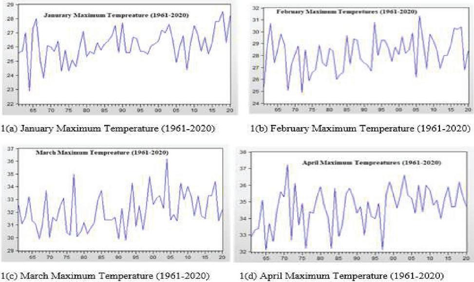
Figure 1 Karachi maximum air temperature January–April (1961–2020).
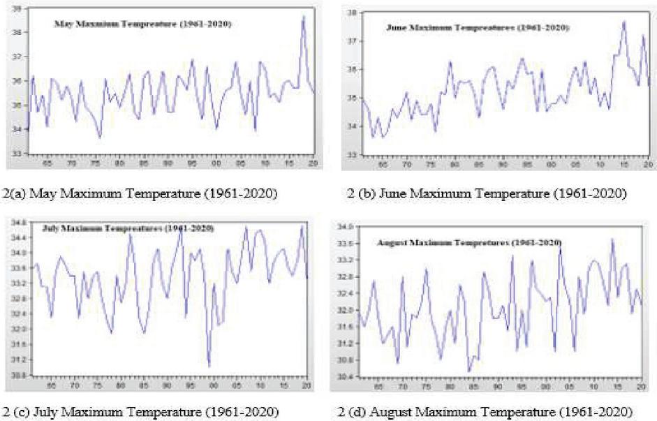
Figure 2 Karachi maximum air temperature May–August (1961–2020).
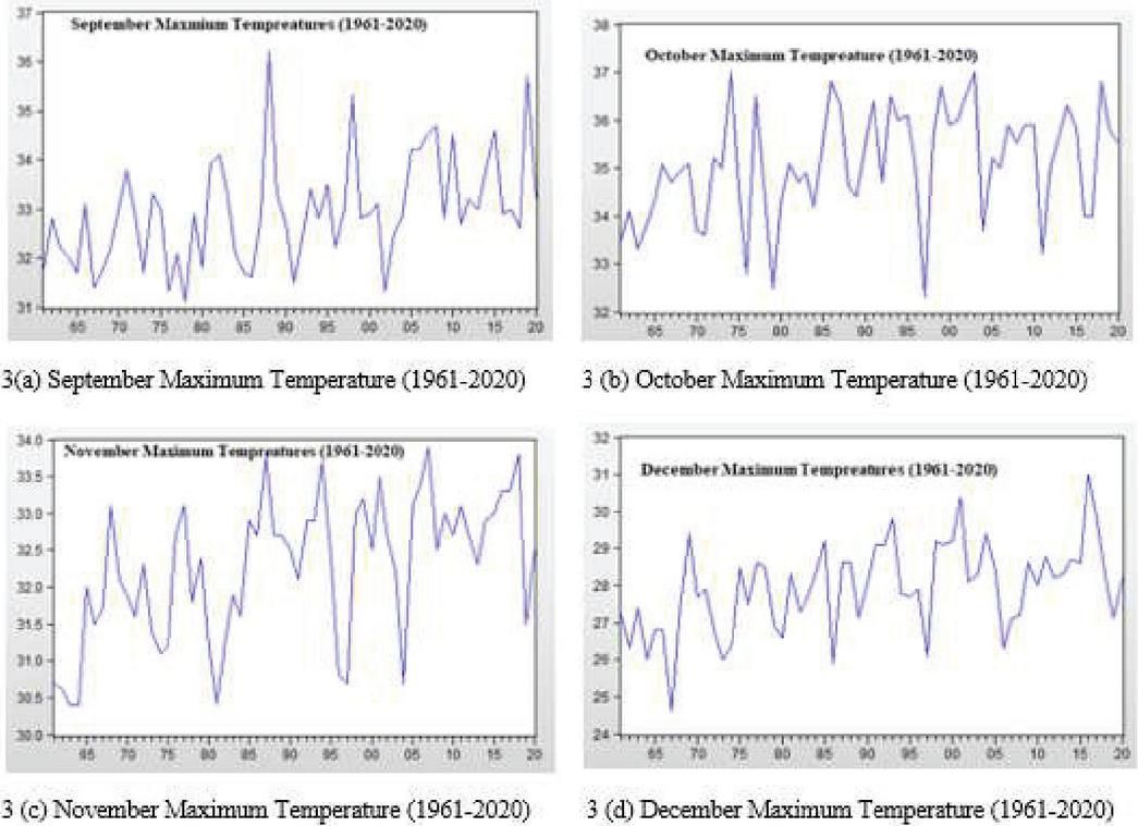
Figure 3 Karachi maximum temperature September–December (1961–2020).
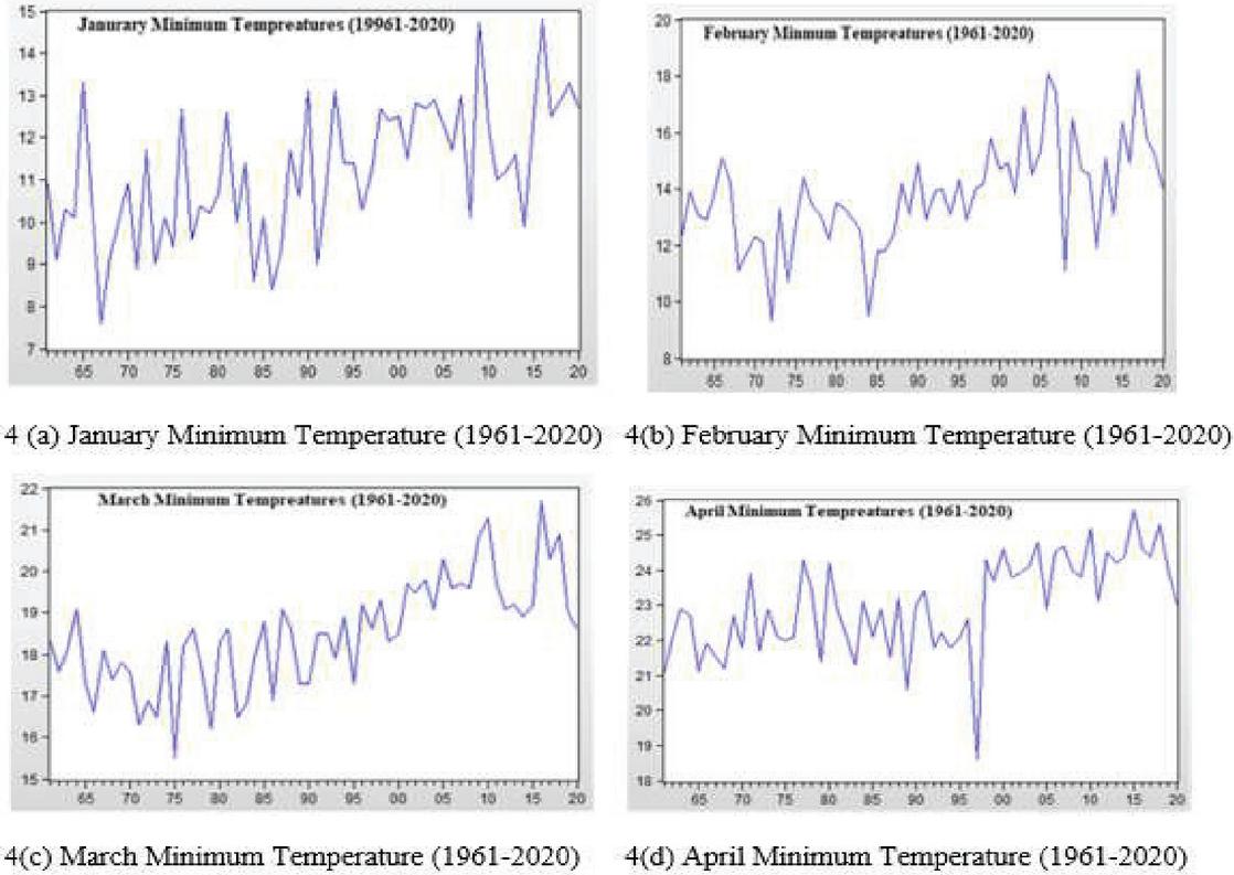
Figure 4 Karachi minimum temperature January–April (1961–2020).
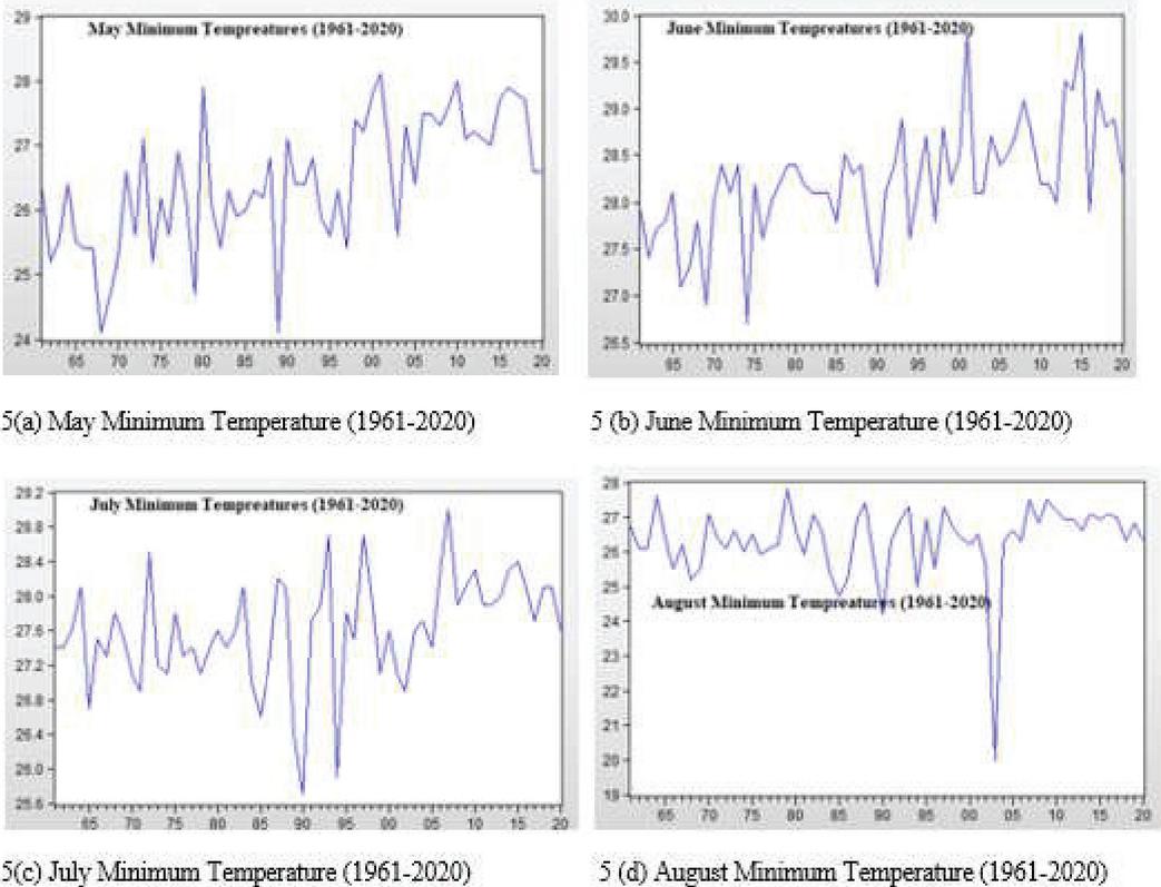
Figure 5 Karachi minimum air temperature May–August (1961–2020).
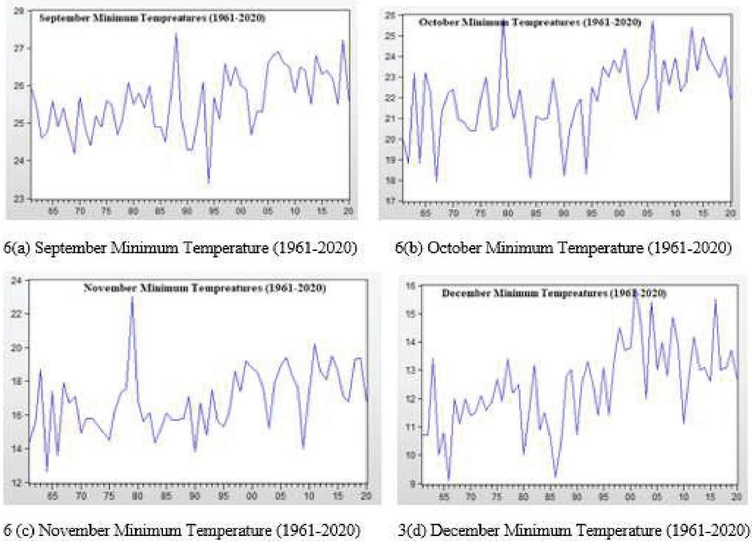
Figure 6 Karachi minimum air temperature September–December (1961–2020).
4 Conclusions
An increase in the average global temperature is referred to as global warming and climate change. This rise in the average worldwide air temperature is mostly caused by natural and human activity. The Earth’s geology will be altered in addition to the water and atmosphere due to the increasing emissions of carbon dioxide from companies, power plants, and cars, which is the source of the climate change. The air temperature is expected to rise by 2 to 6 degrees Celsius by the year 2100 as a result of carbon dioxide emissions brought on by our use of fossil fuels. This is a significant increase from the present average air temperature of 1.7 degrees Celsius, as predicted.
The experiment’s initial goal was to determine how the mean monthly air temperature in Karachi behaves in terms of both maximum and lowest temperatures and climate change. The behavior of the maximum and lowest air temperatures in Karachi is modelled and forecasted using the ARMA (p, q) model. In this context, the data being examined are Karachi’s mean monthly maximum and minimum air temperatures, broken down by month, from 1961 to 2020. Each month’s descriptive studies from 1961 to 2020 are explained. The least values of the Hannan Quinn (HIC), Bayesian Schwarz (SIC), and Akaike (AIC) information criteria are used to determine which models are most acceptable. The Durbin-Watson Test is also useful for determining the best model. The best-fitted model of the mean monthly maximum and minimum air temperature in Karachi is used to determine the forecast accuracy. The metrics used to compute this include root mean square error (RMSE), mean absolute error (MAE), mean absolute percentage error (MAPE), and Theil’s U-Statistics.
With the exception of January, when the best fitted model is ARMA (3, 3), April displays the most fitted model is ARMA (2, 3), and October displays the most appropriate model is ARMA (9, 6). Minimum air temperature. Most months follow the most appropriate model is ARMA (1, 1), and some months show the best adequate model is ARMA (2, 2) process. While the majority of the months in the maximum air temperature display the ARMA (3, 3) model as the most suited, the other months express the different ARMA (p, q) process as the best. When compared to other forecast evaluations such as RMSE and MAE, MAPE scores are lower. Theil’s U-Statistics also shows the monthly average and minimum air temperature. There is a high correlation between the air temperature and the preceding month, as seen by the Theil’s U-Statistics values of each month approaching zero. Risks associated with climate change increase when Earth’s global mean air temperature rises, or as global warming occurs. It is also discovered that during the pandemic, even with the suspension of building and transportation, the difference in temperature did not significantly alter, but the quality of the air did. Non-stationarity data is tested using the unit root method. When the p-value is less than 5% or the Augmented Dickey Fuller (ADF) test’s crucial value of absolute value is higher than at the 1% and 5% significance levels, H0 is rejected. The mean monthly maximum and minimum air temperatures in Karachi were found to be stationary in this study. This study also highlights the the innovative aspect of utilizing vast datasets, possibly including those from mobile and multimedia sources, to address a critical environmental issue. It also emphasizes the predictive modelling aspect of your study, which is central to understanding and mitigating global warming effects.
Acknowledgments
The authors are thankful to the Pakistan Meteorological Department to provide the data of maximum and minimum temperature of Karachi.
The datasets generated during the current study are not publicly available due to Pakistan meteorological department sells the said data but are available from the corresponding author on reasonable request.
References
[1] Sagheb A, Vafaeihosseini E, and P Ramancharla (2011) The Role of Building Construction Materials on Global Warming. Lessons for Architects.
[2] Dawn News (2020) Rising temperatures continue to cause heatwaves. UN – Newspaper – DAWN.COM Karachi,.
[3] News report (2021) Impact of Climate Change on Karachi May be One of Pakistan’s Biggest Threats – Pakistan |ReliefWeb OCHA https://reliefweb.int/report/pakistan/impact-climate-change-karachi-may-be-one-pakistan-s-biggest-threats (2021).
[4] New report (2021) the building and construction sector can reach net zero carbon emissions by 2050 |World Green Building Council https://www.worldgbc.org/news-media/WorldGBC-embodied-carbon-report-published.
[5] New report (2021) Hottest day in history Karachi breaks 74-yr old record with 44 degree temps – Pakistan – Dunya News https://dunyanews.tv/en/Pakistan/595585-Hottest-day-history-Karachi-breaks-74-yr-old-record-44-degree.
[6] Arsalan S (2020) International Journal of Human Capital in Urban Management Greenhouse gasses emission in the highly urbanized city using GIS-based analysis Int. J. Hum. Cap. Urban Manag., 5(4): 353–360, doi: 10.22034/IJHCUM.2020.04.07.
[7] Forster PM (2020) Current and future global climate impacts resulting from COVID-19 Nat. Clim. Chang 10(10): 913–919, doi: 10.1038/s41558-020-0883-0.
[8] Bauwens M (2020) Impact of Coronavirus Outbreak on NO2 Pollution Assessed Using TROPOMI and OMI Observations Geophys. Res. Lett., 47(11): e2020GL087978, doi: 10.1029/2020GL087978.
[9] Zhang R, Zhang Y, Lin H, Feng X, Fu TM, Wang Y (2020) NOx emission reduction and recovery during COVID-19 in East China Atmosphere (Basel) 11(4): 433–440 doi: 10.3390/ATMOS11040433.
[10] Quéré CL (2020) Temporary reduction in daily global CO emissions during the COVID-19 forced confinement Nat. Clim. Chang., 10(7): 647–653, doi: 10.1038/s41558-020-0797-x.
[11] Hassan SA, Nosheen M (2001) The Impact of Air Transportation on Carbon Dioxide, Methane, and Nitrous Oxide Emissions in Pakistan: Evidence from ARDL Modelling Approach Int. J. Innov. Econ. Dev. 3(6): 7–32, Feb. 2018, doi: 10.18775/ijied.1849-7551-7020.2015.36.
[12] Akaike H (1987) Factor Analysis and AIC Springer, New York, NY, 371–386.
[13] Time Series Modelling of Water Resources and Environmental Systems, 45 – 1st Edition 2013. https://www.elsevier.com/books/time-series-modelling-of-water-resources-and-environmental-systems/hipel/978-0-444-89270-6 (2021).
[14] Adhikari R, Agrawal RK (2013) An Introductory Study on Time Series Modeling and Forecasting Feb., Accessed: [Online]. Available: http://arxiv.org/abs/1302.6613 Apr. 07, (2021).
[15] Jenkins JM, Milholland RD, Lilly JP, Beute MK (1970) Commercial gladiolus production in North Carolina NC Univ Ext Circ, Accessed: Apr. 07, 2021. [Online]. Available: https://agris.fao.org/agris-search/search.do?recordID=US201301137874.
[16] Schwabe SH (1843) Die Sonne Astron. Nachrichten, 20 17: 283–286, doi: 10.1002/asna.18430201706.
[17] Hipal KW, Mcleod AI (1994) Time Series Modeling of Water Resources and Environmental System. Amsterdam Elsevier p. 1013.
[18] McCarthy D (2015) An Introduction to Testing for Unit Roots Using SAS The Case of US National Health Expenditures.
[19] da Silva Lopes AC (2006) Deterministic seasonality in Dickey–Fuller tests should we care?. Empirical Economics, 31(1): 165–182.
[20] Yonus, M., and Hassan, S. A. (2022). The Impact of Climate Change on Stochastic Variations of the Hydrology of the Flow of the Indus River. Slovak Journal of Civil Engineering, 30(1), 33–41.
[21] Chien, F., Sadiq, M., Nawaz, M. A., Hussain, M. S., Tran, T. D., and Le Thanh, T. (2021). A step toward reducing air pollution in top Asian economies: The role of green energy, eco-innovation, and environmental taxes. Journal of environmental management, 297, 113420.
[22] Asma Z, Aalim Hussain (2022). Modeling and prediction of KSE 100 index closing based on news sentiments: an applications of machine learning model and ARMA (p, q) model Multimedia Tools and Application, 81(9), 1–23, ISSN: 1380-7501.
[23] Asma Z, Shaheen A, Rashid K. A. (2019) An Analysis of Heavy Tail and Long-Range Correlation of Sunspot and El Nino-southern oscillation (ENSO) Cycles. Solar System Research 53(5). 99–103.
Biographies

Asma Zaffar received the bachelor’s degree, M. Phil and Ph.D. entitled Morphology and image analysis of some solar photospheric phenomena in Mathematics from University of Karachi. Currently serve as an Associate Professor and Chairperson of the department of Mathematics and Sciences, Sir Syed University of Engineering and Technology. She has been HEC approved supervisor from 2019 and published numerous research articles in different national and international reputed journals. Her research area is Time series analysis, Astrophysics, Data Analysis, Homological Algebra and Climate Change.

Shakil Ahmed was born in Karachi, Pakistan dated March 7th, 1980. He received MS degree in Computer Systems Engineering in 2006 and BS degree in Computer Engineering in 2003. He completed his PhD in Computer and Communication System Engineering from University Putra Malaysia in 2014. He has authored and coauthored 20 research papers in various journals and conferences of international repute. He is also a life member of Pakistan Engineering Council. He is currently associated with Sir Syed University of Engineering & Technology as Associate Professor, and also acting as Chairman of Department of Computer Engineering. He is also HEC approved supervisor for PhD candidates. Under his supervision, five candidates are pursuing their PhD and two candidates are doing MS thesis. Apart from chairing the department, he is also heading the Centre for Guidance, Career Planning and Placement Centre as Director since last seven years. His primary research areas are Information Security, Cryptography and Data Mining.

Ayesha Rafique received the bachelor’s degree in Electronic Engineering from NED University of Engineering and Technology in 2010, the Masters degree in Telecommunication Engineering from Hamdard University in 2015. Currently a PhD candidate in Sir Syed University of Engineering and Technology in department of Computer Engineering. She is currently working as senior Lecturer at department of Telecommunication Engineering in Sir Syed University of Engineering and Technology. Her research areas include deep learning, Climate Smart Agriculture, Neural networks and Climate change.

Muhammad Imran did PhD from Universiti Teknologi PETRONAS Perak, Malaysia. Muhammad has 11+ years of experience as a Researcher and Structural Design Engineer. He has designed, repaired damaged structures and did the forensic analysis for O&G facilities after fire accidents. His current research is on Structural fire safety and building material and strengthening. His MS project was on the strengthening of reinforced concrete beams using CFRP.

Muhammad Aamir received an MS degree in Electronic Engineering (with specialization in Telecommunication) in 2002 and a BS in Electronic Engineering in 1998 from Sir Syed University of Engineering and Technology Karachi. He accomplished his PhD in Electronic Engineering from Mehran University of Engineering & Technology Jamshoro in December 2014. During his PhD studies, he accomplished major part of his research work at the University of Malaga Spain under Erasmus Mundus Scholarship. He has authored and co-authored around 50 research papers and book chapters published in various journals, books and conferences of international repute including more than 15 papers with co-authorship of Professors from Mehran University of Engineering & Technology. He is a life member of Pakistan Engineering Council and senior member of IEEE and currently serving as chair of IEEE Communication Society for Karachi Chapter. He was awarded with a grant by the Ministry of Education Spain to teach at the University of Malaga which he successfully availed in May 2012. He had also served as Member of two separate National Curriculum Revision Committees constituted by Higher Education Commission (HEC) for revision of Electronic Engineering Curriculum and Telecommunication Engineering Curriculum at the National Level. He is currently associated with Sir Syed University of Engineering & Technology as Professor and Dean in the Faculty of Electrical & Computer Engineering. Additionally, he is also Editor-in-Chief of Sir Syed University Research Journal of Engineering & Technology (HEC Recognized Journal) which is published bi-annually. He has been included in the Stanford University’s top 2% global scientists list. The US-based Stanford University released a list in October 2020 that represents the top 2% of the most-cited scientists in multiple disciplines. The list comprises around 160,000 persons from all over the world while only 243 Pakistani were included in the list so it is a unique honor that an alumni of Sir Syed University of Engineering & Technology is recognized at International level within top 2% global scientists in multidisciplinary research.

Vali Uddin Presently serving as Vice Chancellor, Sir Syed University of Engineering & Technology, Karachi. Vali Uddin earlier served at Hamdard University, Karachi, as Professor, (July 2011 – June 2019), Acting Vice Chancellor (from October 24 till October 31, 2013, and July 22, 2014 till August 29, 2014), Dean, Faculty of Engineering Sciences and Technology (July 2013 – May 2019), Registrar (April 2017 till October 2018), Acting Registrar, (August 2012 till August 2015) and, Director, Hamdard Institute of Information Technology, (July 2011 – July 2013). Vali Uddin earned his Ph.D. Electrical Engineering from Boston University, MA, USA.
Earlier, he did his BE (Electronics) from NED University, Karachi with First Class First Position and went on to do his MS Electrical Engineering from Boston University, Boston, MA. He was Conference Chairman of First and Second IEEE International Conference on Computer Control and Communication at PNEC-NUST, Karachi on 12–13 November 2007 and 17–18 February, 2009 respectively and Conference General Chair of 21st IEEE International Multi-topic Conference, Hamdard University Karachi held on November 01–02, 2018. He initiated BE (Electronics), BE (Telecommunication), MS (Computer Science), MS (Engineering), PhD (Computer Science) and PhD (Engineering) degree programs at Iqra University, Karachi as a Dean, Faculty of Engineering, Sciences and Technology. He initiated BE (Electrical) and BE (Mechanical) degree programs at Hamdard University as Dean, Faculty of Engineering, Sciences and Technology. He has been a key member of a team as Registrar who brought Financial turnaround of Hamdard University in less than two years. He has been a key member of a team member who developed and expanded MS and PhD programs at PNEC-NUST.
Journal of Mobile Multimedia, Vol. 20_6, 1289–1320.
doi: 10.13052/jmm1550-4646.2065
© 2025 River Publishers