Evaluation of UHF Transfer Function in a Power Transformer for Real-Time Partial Discharge Detection

Sathaporn Promwong* and Thanadol Tiengthong

Faculty of Engineering, King Mongkut’s Institute of Technology Ladkrabang, Ladkrabang, Bangkok, 10520, Thailand

E-mail: sathaporn.pr@kmitl.ac.th; 60601188@kmitl.ac.th

* Corresponding Author

Received 30 April 2020; Accepted 31 May 2020; Publication 17 August 2020

Abstract

The UHF transfer function is significant for a short-range communication system, e.g., a real-time diagnosis of partial discharge (PD). Real-time diagnosis of the PD has become a challenging topic of improving the diagnosis of high voltage equipment, including a power transformer. Further, the PD detection in high voltage equipment is critical since the PD can cause severe damage to electrical systems. The PD detection methods are classified by a phenomenon of the PD. The PD detection by electromagnetic (EM) method is regulated by IEC TS 62478, which specified the UHF band for the PD detection in power transformers. Hence, an evaluation of frequency characteristics is essential to achieve an excellent diagnostic performance. In this paper, a complex form of channel analysis is applied with the PD detection method. The measurement model in a power transformer is proposed. The optimum receiver is introduced to maximize SNR and hence it is easy to analyze the results. The results were analyzed by using magnitude, phase, group delay, received waveform, and path loss parameters. The results show that the measured channel is affected by the structure of the power transformer. The contribution of this research is useful for improving the precision of the PD detection with EM method and building an accurate real-time partial diagnosis via a smartphone or laptop computer.

Keywords: UHF, complex form, UHF transfer function, Friis’ transmission formula, partial discharge.

1 Introduction

Short-range multimedia technology and wireless communications have rapidly developed in recent years. It can apply to various applications, such as wireless sensors network and the internet of things (IoT) [1–3]. Ultra-high frequency (UHF) is usually used for video and sound broadcasting, mobile communications, Wi-Fi, and numerous kinds of applications [4]. The theory of wireless communications can be adapted to analyze the problems in the majority of the novel applications, e.g., wireless sensor networks, near-field communications, wireless access networks, field intensity in an inhomogeneous propagation environment [5–9], and wireless transformer condition diagnosis with electromagnetic method [10]. Partial discharge (PD) real-time diagnosis is one of the ways which can develop due to the benefit of the advanced investigation in wireless communications and partial diagnosis. Real-time diagnosis can help a maintenance operator to identify a problem without entering an actual site.

Further, the PD diagnosis is critical to avoid the undesired damage to a power system [11]. The PD may occur in various places, i.e., GIS, switchgear, and power transformer [12]. An antenna is used as a probe for the PD diagnosis to investigate the PD in the power transformer with an electromagnetic method [13]. The antenna’s properties are taken into account to assess the antenna’s performance so as to satisfy the condition of PD diagnosis in power transformers with the electromagnetic method. The minimum of interference in the sensor affects efficiency for short-range communication applications. It has attracted the majority of attention to investigate the sensor transfer function [14–20].

In the power transformer system, the PD and antennas are behaving like the pulse-shaping filter. The pulse shape of the transmission signal can be affected by the pulse shape distortion that is caused by any signal distortion in the frequency domain. Therefore, the complexity of the receiver mechanism will increase. A typical transformer is a request for a suitable structure, reasonable cost, and excellent performance. Hence, the design of the antenna for PD diagnosis in the transformer is one of the attractive challenges [13–20]. The Friis’ transmission formula could not be directly used to diagnose the PD in the transformer, due to the signal’s pulse shape, even though it is in line with sight. Therefore, the UHF signal waveform comparison is essential due to the Fresnel region of the antenna frequency response.

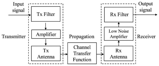
Figure 1 UHF communications system [4].

The antenna’s properties are measured and discussed in this paper. The antenna transfer function in the Fresnel region is evaluated to investigate the PD propagation in the transformer. The modification of the Friis’ transmission formula is introduced as the complex form equation for the PD diagnosis in the transformer. For this reason, the equivalent antenna gain had been derived. The transmission waveform and the optimum filter at the receiver are the primary modifications for the complex form of the Friis’ transmission formula for the PD diagnosis in the transformer. The experiment had been done by using the UHF microstrip patch antenna for 2.2 GHz to 2.6 GHz band operation in the power transformer. The evaluation system in this paper is based on the UHF communications system, which is shown in Figure 1.

2 Partial Discharge

The PD is a phenomenon which occurs by the partial bridge of the electrical discharge between the insulation of the conductors. It can be observed in various high voltage equipment, e.g., the power transformer, GIS, and rotating machines. It is essential to understand the phenomenon of the PD since it can lead to power breakdown in power systems. The International Electrotechnical Commission (IEC) has regulated the PD definition in the IEC 60270:2000 standard [10]. The general descriptions and measuring systems have been documented. This activity is generally caused by the electrical stress concentration in the insulation of the electrical devices. The PD is related to the conditions of the insulation of the high voltage equipment, i.e., charge transportation, chemical reaction, light emission, sound release, and the radiation of electromagnetic waves.

According to different types of the conditions, the PD test methods of parts can be separate due to the circumstances [11], e.g., gas analysis for the chemical reaction, optical measurements for the light emission, the electrical measurement for the charge transport, the acoustic measurement for the sound release, and the electromagnetic measurement for the radiation of the electromagnetic wave. The PD test technique has been stated in the IEC standard, i.e., the IEC 60207:2000 for the PD measurement and the IEC TS 62478:2016 for the analysis of PDs by the electromagnetic and acoustic methods [12]. Following the IEC TS 62478:2016 standard, the short rise time of the PD pulse current is less than 1 ns. The pulse can be ranging from 3 MHz to 3 GHz. The advantages of the electromagnetic method are that it is better immune to disturb and noise, in determining a characteristic of the PD source, and in broad bandwidth. However, some disadvantages of the electromagnetic method, i.e., high equipment cost and the performance of this method, tend to rely on the physical structure of the sensors. There are various types of sensors available for detecting the PD pulse, for example, UHF antenna, disc- and cone-shaped sensors, field grading electrode, wave guild sensor, and directional electromagnetic couplers. The sensor output can indicate the importance of many parameters, e.g., transfer function, frequency characteristics, field magnitude dependence, and directional characteristics. The localization of the PD sensor is significant. The sensor can be installed inside the high voltage equipment. It should be installed as close as to the high voltage component area or the PD detection area.

The propagation mechanism easily influences the PD pulse characteristics effects such as diffraction, reflection, scattering, and attenuation. This interference is causing disturbances in the measurement of PDs with the electromagnetic method. Therefore, to decrease the interference from the ambient environment in the measurement of PDs, the analysis of the characteristic of the transfer function in the measuring environment is necessary.

3 Complex Form Analysis for the PD Detection in a Power Transformer

The Friis’ transmission formula is the first to express in terms of power [21]. Then it is extended in terms of the transmission signal waveform to consider the transfer function [22–24]. It is assumed that the polarization of the transmitter antenna and receiver antenna match correctly. A block diagram of the PD UHF system for complex form analysis is shown in Figure 2.

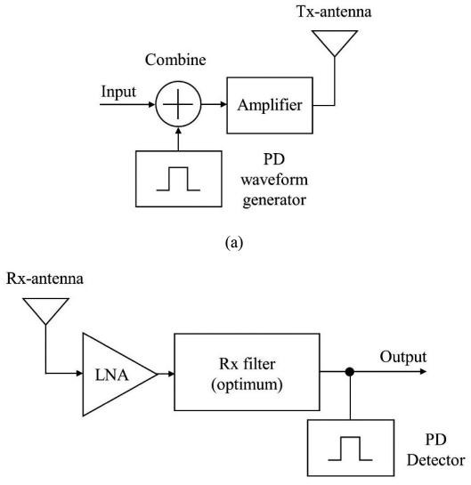
Figure 2 Block diagram of the PD UHF transceiver model: (a) PD UHF transmitter and (b) PD UHF receiver with optimum filter.

Equation (1) is the modification of the Friis’ transmission formula. It includes three elements, namely the frequency characteristics of the antennas, the frequency characteristics of free space propagation, and the spectrum of the transmitted signal. The PD UHF channel corresponding transfer function H_ch−corr(f, R) is

$$H_{\mathrm{ch}-\mathrm{corr}}(f,R)=H_{\mathrm{f}}(f,R)H_{\mathrm{r}}(f)H_{\mathrm{t}}(f),$$

(1)

where H_f(f, R) is the transfer function of the free space, H_r(f) and H_t(f) are the transfer functions of the transmitter (Tx) and the receiver (Rx) antennas. Furthermore, R is the transmitter antenna and receiver antenna (Tx-Rx) separation distance. The transfer function of the free space can be written as

$$H_{\mathrm{f}}(f,R)=\frac{c}{4\pi |f|R}\exp (-jkR),$$

(2)

which is the free space transfer function where

$$k=\frac{2\pi f}{c}$$

(3)

where k is the propagation constant, c is the speed of propagation, and f is the operating frequency. The received waveform v_r(t, R) can be found by using

$${\nu }_{\mathrm{r}}(t,R)=v_{\mathrm{t}}(t)\otimes h_{\mathrm{ch}-\mathrm{corr}}(t,R),$$

(4)

where ν_t(t) is the transmitted signal waveform, ⊗ is the convolution operator, and h_ch−corr(t, R) is the impulse response of the modification of the Friis’ transmission formula defined as

$$h_{\mathrm{ch}-\mathrm{corr}}(t,R)=F^{-1}\{H_{\mathrm{ch}-\mathrm{corr}}(f,R)\},$$

(5)

where F⁻¹ {·} is the inverse Fourier transform (IFFT). The receiver spectrum density V_r(f) is presented as

$$V_{\mathrm{r}}(f)=V_{\mathrm{t}}(f)H_{\mathrm{ch}-\mathrm{corr}}(f),$$

(6)

where the spectrum density of the transmission waveform is V_t(f).

3.1 Optimum receiver

The transfer function of the UHF channel measurement with the optimum receiver filter is H_opt(f). The optimum filter has been introduced in the system to maximize the signal-to-noise ratio (SNR) of the receiver, as shown in Eq. (7)

$$H_{\mathrm{opt}}(f)=\frac{H_{\mathrm{ch}-\mathrm{corr}}^{\ast }(f)}{\sqrt{{\int }_{-\mathrm{\infty }}^{\mathrm{\infty }}{\left|H_{\mathrm{ch}-\mathrm{corr}}^{\ast }\right|}^2\mathrm{d}f}},$$

(7)

and for the prediction case

$$H_{\mathrm{opt},\mathrm{p}}(f)=\frac{H_{\mathrm{ch}-\mathrm{corr},\mathrm{p}}^{\ast }(f)}{\sqrt{{\int }_{-\mathrm{\infty }}^{\mathrm{\infty }}{\left|H_{\mathrm{ch}-\mathrm{corr},\mathrm{p}}^{\ast }\right|}^{2}df}},$$

(8)

which satisfies the following constant noise output power condition

$${\int }_{-\mathrm{\infty }}^{\mathrm{\infty }}{|H_{\mathrm{ch}-\mathrm{corr}}(f)|}^2\mathrm{d}f=1.$$

(9)

The output waveform and the spectrum of the receiver output are h_ch−corr(t, R) and H_ch−corr(f, R), respectively. For the spectrum of the output from the optimum filter V_opt(f)

$$\begin{array}{r}\begin{array}{rl}{V}_{\mathrm{opt}}(f)& =H_{\mathrm{ch}-\mathrm{corr}}(f)H_{\mathrm{opt}}(f)\\ & =\frac{{|H_{\mathrm{ch}-\mathrm{corr}}(f)|}^2}{\sqrt{{\int }_{-\mathrm{\infty }}^{\mathrm{\infty }}{|H_{\mathrm{ch}-\mathrm{corr}}(f)|}^2\mathrm{d}f}},\end{array}\end{array}$$

(10)

and the waveform of the output from the optimum filter ν_opt(t) is

$$\begin{array}{r}\begin{array}{rl}{\nu }_{\mathrm{opt}}(t)& =h_{\mathrm{ch}-\mathrm{corr}}(t)\otimes h_{\mathrm{opt}}(t)\\ & =\frac{h_{\mathrm{ch}-\mathrm{corr}}(t)\otimes h_{\mathrm{opt}}(-t)}{\sqrt{{\int }_{-\mathrm{\infty }}^{\mathrm{\infty }}{h}_{\mathrm{ch}-\mathrm{corr}}^2(t)\mathrm{d}t}},\end{array}\end{array}$$

(11)

and the prediction case

$$\begin{array}{r}\begin{array}{rl}{\nu }_{\mathrm{opt},\mathrm{p}}(t)& =h_{\mathrm{ch}-\mathrm{corr},\mathrm{p}}(t)\otimes h_{\mathrm{opt},\mathrm{p}}(t)\\ & =\frac{h_{\mathrm{ch}-\mathrm{corr},\mathrm{p}}(t)\otimes h_{\mathrm{opt},\mathrm{p}}(-t)}{\sqrt{{\int }_{-\mathrm{\infty }}^{\mathrm{\infty }}{h}_{\mathrm{ch}-\mathrm{corr},\mathrm{p}}^2(t)\mathrm{d}t}},\end{array}\end{array}$$

(12)

and finally, we get the maximum as

$$\begin{array}{r}\begin{array}{rl}max{\nu }_{\mathrm{opt}}(t)& ={\int }_{-\mathrm{\infty }}^{\mathrm{\infty }}{V}_{\mathrm{opt}}(f)df\\ & =\sqrt{{\int }_{-\mathrm{\infty }}^{\mathrm{\infty }}{|H_{\mathrm{ch}-\mathrm{corr}}(f)|}^{2}df}\end{array}.\end{array}$$

(13)

The path loss PL_UHF[dB] can be calculated from the obtained transmitted waveform and received waveform. It can be defined in decibels as the ratio between the maximum amplitude of the transmitted waveform and the maximum amplitude of the received waveform as

$$P{L}_{\mathrm{UHF}}[\mathrm{dB}]=10\log {\left(\frac{\left|{\nu }_{\mathrm{r}}\left(t\right)\right|}{|{\nu }_{\mathrm{t}}(t)|}\right)}^2.$$

(14)

4 Measurement System Model

To investigate the complex form of in the power transformer with measured transfer function in this paper, the measurement system model had been provided such that a measurement procedure is divided into two cases. The first case will measure the complex transfer function in the power transformer at different heights of the transmitter (Tx) antenna and receiver (Rx) antenna. Moreover, an analysis is carried out by using the compare magnitude, phase, group delay, and path loss with different antenna heights at 5 cm, 20 cm, 40 cm, 60 cm, and 80 cm. The second case will measure the transfer function in power transformers at different Tx – Rx separation distances. It ranges from 0.05 m to 1.05 m. It analyzes by using the compares of the received waveform and path loss with different antenna separation distances.

The vector network analyzer (VNA) is used to measure and collect the data, where the transmitter antenna is connected to port-1 and the receiver antenna is connected to port-2 of the VNA. The UHF microstrip patch antenna is considered for use in the experiment due to the property of the antenna, which can operate in a wide bandwidth. The measurement had been done in the power transformer with different Tx – Rx antenna heights and distances. The setup of the experimental model is presented in Figure 3. It should be noted that the calibration at connectors and transmission cables had done before initiating the measurement to reduce interference from noise in connectors and transmission cables. In the experiment, the varying separation distance is chosen to determine the accuracy of the transfer function at different reference separation distances. The experimental parameters are shown in Table 1.

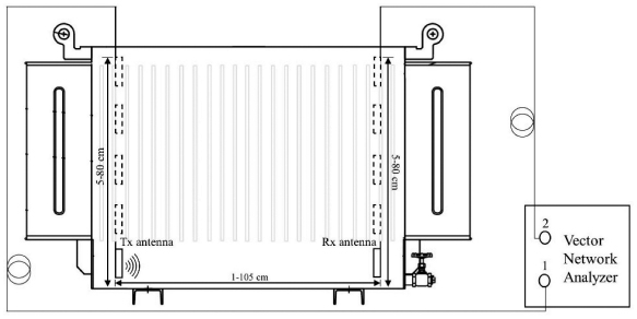
Figure 3 Experimental setup in the power transformer.

Table 1 Example parameters of experiments

Parameters	Values
Frequency range	2.2 GHz to 2.6 GHz
Frequency points	801 points
Tx – Rx antennas type	UHF microstrip patch antenna
Tx – Rx antennas height	5 cm, 20 cm, 40 cm, 60 cm, and 80 cm
Tx – Rx separate distances	0.01 m to 1.05 m

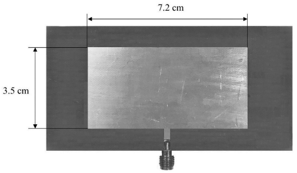
Figure 4 Geometry and dimension of the UHF microstrip patch antenna [26].

4.1 UHF microstrip patch antenna

The Fresnel region of the UHF microstrip patch antenna in this paper is determined from the antenna’s largest dimension for both the transmitter antenna and receiver antenna. The largest dimension of both the transmitter antenna and receiver antenna, as shown in Figure 4, is 8 cm which is considered as the largest dimension of the antenna. The far-field region of the antenna is 40.96 cm, and the far-field can be calculated by Eq. (15) [25]

$$R_{\mathrm{far}}\ge \frac{2D^2}{\lambda },$$

(15)

where

Rfar	is the far-field region,
λ	is the wavelength (m),

and D is the largest dimension of the antennas which can be calculated by Eq. (16)

$$D=D_{\mathrm{Tx}}+D_{\mathrm{Rx}},$$

(16)

where

DTx	is the largest dimension of the transmitter antenna (m) and
DRx	is the largest dimension of a receiver antenna (m).

4.2 Transmission waveform for the UHF PD

This paper considered using the rectangular passband for the signal bandwidth used in the UHF frequency range, i.e., 2.2 GHz to 2.6 GHz. The waveform distortion significantly increases when the bandwidth is larger. The transmitted waveform is presented as

$${\nu }_{\mathrm{t}}(t)=\frac{A}{\mathrm{BW}}[f_{max}\sin c\left(2\pi f_{max}t\right)-f_{min}\sin c\left(2\pi f_{min}t\right)],$$

(17)

$$V_{\mathrm{t}}\left(f\right)=\{\begin{array}{cc}1/2\mathrm{BW}& ||f|-f_{\mathrm{c}}|\le \mathrm{BW}/2\\ 0& ||f|-f_{\mathrm{c}}|>\mathrm{BW}/2\end{array},$$

(18)

where the minimum frequency (f_min) is 2.2 GHz and the maximum frequency (f_max) is 2.6 GHz. The occupied bandwidth is BW, the amplitude is A, the operating frequency is f, and the center frequency is f_c. The transmitted waveform and spectrum density of the transmitted waveform are shown in Figure 5.

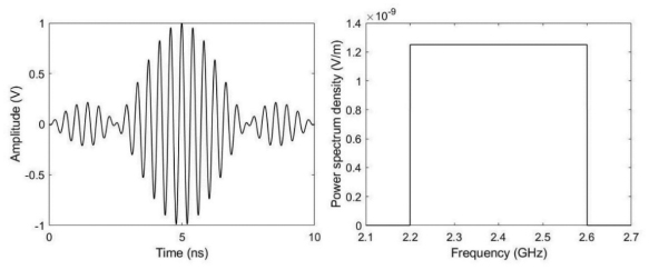
Figure 5 Example transmitted waveform and power spectrum density of UHF systems.

5 Results and Discussions

The measurement of the transfer function in the power transformer was done according to the proposed measurement model, as presented in Section 4. This research was done by dividing a measurement into two cases. The first case is is to present the comparison of magnitude, phase, group delay, and path loss between different Tx – Rx antennas’ height. The second case is to present a comparison of received waveform and path loss between different Tx – Rx antennas’ separation distance. From the results, we can show the different characteristics of the measured transfer function, which we will discuss further.

The channel transfer function of complex form in the power transformer can be easily analyzed using a magnitude. Figure 6 shows the comparison of the magnitude at different Tx – Rx antennas’ height, i.e., 5 cm, 20 cm, 40 cm, 60 cm, and 80 cm. A solid black line, black-dashed line, black-dotted line, black dash-dot line, and the solid gray line represent the magnitude of each antenna’s height, respectively. The results at 5 cm of the antenna’s height show that it has a better magnitude than the other heights of the antenna. The magnitudes of 20 cm, 40 cm, 60 cm, and 80 cm antenna height are similar. However, the magnitude of the 80 cm antenna height is lower than the other antenna height. Besides, many low magnitudes occur due to the structure of the power transformer and noise from the environment.

In Figure 7, a comparison of phase from the Tx – Rx antennas channel transfer function at different antenna heights is provided. The results are presenting by using different types of lines as same as in Figure 6. The phase of 5 cm antenna height is better and has more linearity than other antenna heights. The phase of the antenna is performed in the same direction at the antenna heights of 20 cm, 40 cm, 60 cm, and 80 cm. However, the phases of 20 cm and 60 cm antenna heights have some error due to the noise from the environment. It made the phase of 20 cm antenna height more phase changing in a lower frequency. The phase of 60 cm antenna height has the lowest phase of channel transfer function compared to other antenna heights.

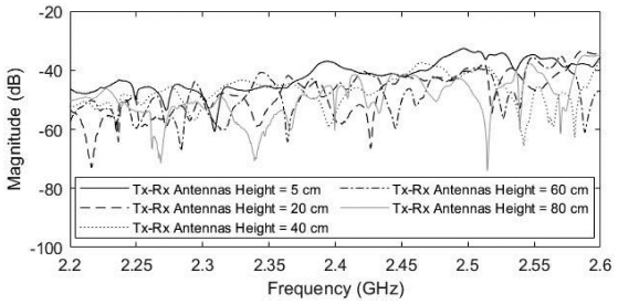
Figure 6 The comparison of magnitude between different Tx – Rx antennas height.

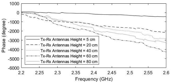
Figure 7 The comparison of phase between different Tx – Rx antennas height.

Group delay is another parameter used in the investigation of complex form analysis with measured transfer function. It is advantageous to present a time distortion and then calculating by differentiating the concerned frequency. In Figure 8, the comparison of the group delay of the measured channel transfer function at different antenna heights is presented. From the results, we now discuss the group delay trends. The group delay of 0 cm antenna height has the lowest delay. The group delay of 80 cm antenna height has the highest delay. The group delay results had shown good agreement with the phase results. Further, some frequencies had high delay due to the noise, the reflection of the waveform, the structure of the power transformer, and the environment.

Figure 9 compares the received waveform between the optimum case and the prediction case of the channel transfer function with a different separation distance of the Tx – Rx antennas. The optimum case is calculated using the measurement data with Eq. (13). The prediction case is calculated by using Eq. (12). The received waveform of prediction and measurement is presented by the black dashed line and solid black line, respectively. The difference between optimum and prediction cases can be presented with the effect of the Fresnel region. In Figure 9(a), the received waveform at 0.3 m distance is presented. It shows a difference in the optimum case and prediction case. At this distance, the optimum received waveform is different from the predicted received waveform due to the near-field region.

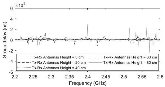
Figure 8 The comparison of group delay between different Tx – Rx antennas height.

On the other hand, Figures 9(b) and 9(c) show the comparison of the received waveform between the optimum and prediction cases at 0.6 m and 0.9 m distances, respectively. At these distances, the measured received waveform and predicted received waveform are almost the same. From these results, we conclude that the received waveform is related to a near-field region of the antenna. However, at 0.6 m and 0.9 m distances, there is a little difference between the measured waveform and prediction waveform. It maybe caused due to the reflection of waveform inside the power transformers and the structure of the power transformer.

The path loss parameter is useful to investigate a power loss concerning the separation distance between the Tx antenna and the Rx antenna. In our research, the measurement model had been designed to analyze the effect of the Tx – Rx antennas’ separation distance in the power transformer. The model was divided into two cases, as presented in the earlier section. The first case is to investigate the difference of path loss at different antenna heights, as presented in Figure 10. The second case is to investigate the difference in path loss between the optimum case and the prediction case, as presented in Figure 11. In Figure 10, the comparison of path loss between different antenna heights is presented. The line style of Figure 10 represented the same meaning as that in Figure 6. It shows that at 5 cm, the antenna height has the lowest path loss compared to other antenna heights. Moreover, the path loss of 20 cm, 40 cm, 60 cm, and 80 cm antenna heights are close to each other and higher than the path loss of 5 cm antenna height.

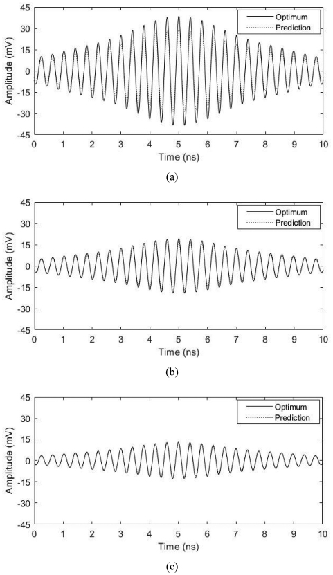
Figure 9 The received waveform of UHF transfer function at (a) 0.3 m, (b) 0.6 m, and (c) 0.9 m.

In Figure 11, for example, the path loss at the Tx – Rx antennas height of 5 cm is present because at this height the path loss has been less than the others. The comparison of optimum path loss and prediction path loss is presented. The relation path loss due to the far-field region of the antennas is presented by the solid black line and black-dashed line, respectively. The results present a considerable difference in path loss at the far-field region of the antenna. The difference will reduce when the antenna separation distance is further than the Fresnel region of the antenna. The comparison of path loss at 5 cm of the antenna height is given in Table 2. It shows an error between the optimum path loss and the prediction path loss. At the antenna separation distance of 0.3 m, the path loss error is 2.43 dB. The path loss error at the antenna separation distances of 0.6 m and 0.9 m is 1.11 dB and 0.70 dB, respectively, due to the effect of the antennas’ far-field region. The results show that the proposed method can be used to evaluate the UHF transfer function. It will be also useful for application in real-time PD detection and other wireless sensor networks applications.

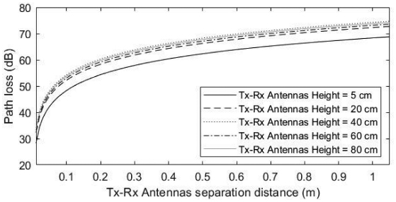
Figure 10 The comparison of path loss between different Tx - Rx antennas height.

Figure 11 The comparison of path loss of the measured transfer function at Tx – Rx antennas height of 5 cm.

Table 2 The comparison of path loss at Tx – Rx antenna separation distances at 0.3 m, 0.6 m, and 0.9 m with Tx – Rx antennas height of 5 cm.

	Path loss at Tx – Rx antennas separation distance
	0.3m	0.6m	0.9 m
Prediction	61.65 dB	66.36 dB	69.47 dB
Measurement	59.22 dB	65.25 dB	68.77 dB
Error	2.43 dB	1.11 dB	0.70 dB

6 Conclusion

In this paper, the explanation of how to evaluate the complex transfer function in the power transformer with the measured transfer function had been presented for application in real-time PD detection. The modification of the Friis’ transmission formula has been used to consider the transfer function measurement in the power transformer channel model. The measurement model has been tested in a real power transformer of the Tesla Power Co., Ltd. The error in complex form in the power transformer had observed by changing the Tx – Rx antennas’ height and Tx – Rx antennas’ separation distance. The measurement had been done with two UHF microstrip patch antennas which represent the Tx – Rx antennas and record the measured data with the VNA. The calibration had done at the connector and transmission cables before the measurement. The results of the complex form analysis are presented as two different cases. The first case is presented as the comparison of magnitude, phase, group delay, and path loss between different heights of the Tx – Rx antennas. It shows that the lower antenna height has better results than the higher antenna height due to the noise and power transform structure. The second case is presented as the comparison of near-field and far-field between the received waveform and path loss. The latter case shows that the near-field region has an error more than the far-field region due to the radiation field. In conclusion, this paper presents the analysis of the complex form with the measured transfer function. It can be useful for designing realtime PD detection systems in the power transformer and other short-range wireless systems.

Acknowledgments

The authors would like to thank Dr. Norasage Pattanadech, Dr. Chanin Bunlaksananusorn, and Dr. Pichaya Supanakoon from KMITL for support the experimental and reviewing on our manuscript. We would also like to thank Mr. Sakda Maneerot from the Tesla Power Co., Ltd., for allowing us to use the power transformer.

References

[1] Q. Huang and K. Kietter, “An intelligent internet of things (IoT) sensor system for building environment monitoring,” Journal of Mobile Multimedia, vol. 15, no. 1–2, pp. 29–50, January 2019.

[2] F.D. Miyandoab, J.C. Ferreira, and V.M.G. Tavares, “Analysis and evaluation of an energy-efficient rotating protocal for WSNs combining source routing and minimum cost forwarding,” Journal of Mobile Multimedia, vol. 14, no. 4, pp. 469–504, October 2018.

[3] C. Pham, N.N. Diep, and T.M. Phuong, “A wearable sensor based approach to real-time fall detection and five-grained activity recognition,” Journal of Mobile Multimedia, vol. 9, no. 1–2, pp. 15–26, November 2013.

[4] A. Graham, N. C. Kirkman, and P. M. Paul, “Mobile radio network design in the VHF and UHF bands: a practical approach,” West Sussex, England: John Wiley & Sons, 2007.

[5] W. Narzt, L. Furtmuller, and M. Rosenthaler, “Is Bluetooth low energy an alternative to near-field communication,” Journal of Mobile Multimedia, vol. 12, no. 1–2, pp. 76–90, April 2016.

[6] D. Benhaddou and J. Naraujo, “Field measurement of an urban two-tier wireless mesh access network: end-user perspective,” Journal of Mobile Multimedia, vol. 10, no. 1–2, pp. 141–159, May 2014.

[7] J. Honda, K. Uchida, and M. Takematsu, “Analysis of field intensity distribution in inhomogeneous propagation environment based on two-ray model,” Journal of Mobile Multimedia, vol. 8, no. 2, pp. 88–104, June 2012.

[8] J. Shi, K. Cai, C. He, G. Wei, and Z. Shan, “An energy-adaptive path routing approach for wireless sensor networks,” Journal of Mobile Multimedia, vol. 8, no. 1, pp. 34–48, April 2012.

[9] A. Setyini, M.J. Alam, and C. Eswaran, “Study and development of the transmission method for large multimedia file size using multimedia messaging service technology,” Journal of Mobile Multimedia, vol. 8, no. 1, pp. 1–24, April 2012.

[10] J. Du, W. Chen, L. Cui, Z. Zhang, and S. Tenbohlen, “Investigation on the Propagation Characteristics of PD-Induced Electromagnetic Waves in an Actual 110 kV Power Transformer and Its Simulation Results,” IEEE Transactions on Dielectrics and Electrical Insulation, Vol. 25, No. 5, pp. 1941–1948, October 2018.

[11] IEC Standard 60270, “Partial discharge measurement,” 3rd Edition, International Electrotechnical Commission, Geneva, Switzerland, 2000.

[12] Cigré 502, “High-voltage onsite testing with partial discharge measurement,” Conseil International des Grands Réseaux Électriques, France, 2012.

[13] IEC/TS Standard 62478, “High voltage test techniques – Measurement of partial discharge by electromagnetic and acoustic methods,” International Electrotechnical Commission, Geneva, Switzerland, 2016.

[14] S. Tenbohlen, D. Denissov, and S. M. Hoek, “Partial discharge measurement in the ultra high frequency (UHF) range,” IEEE Transactions on Dielectrics and Electrical Insulation, vol. 15, no. 6, pp. 1544–1552, December 2008.

[15] M. Hikita, S. Ohtsuka, J. Wada, S. Okabe, T. Hoshino, and S. Maruyama, “Study of partial discharge radiated electromagnetic wave propagation characteristics in an actual 154 KV model GIS,” IEEE Transactions on Dielectrics and Electrical Insulation, vol. 19, no. 1, pp. 8–17, 2012.

[16] T. Li, X. Wang, C. Zheng, D. Liu, and M. Rong, “Investigation on the placement effect of UHF sensor and propagation characteristics of PD induced electromagnetic wave in GIS based on FDTD method,” IEEE Transactions on Dielectrics and Electrical Insulation, vol. 21, no. 3, pp. 1015–1025, 2014.

[17] W. Gao, D. Ding, W. Liu, and X. Huang, “Investigation of the evaluation of the PD severity and verification of the sensitivity of partial-discharge detection using the UHF method in GIS,” IEEE Trans. Power Del., vol. 29, no. 1, pp. 38–47, 2014.

[18] R. Rostaminia, M. Saniei, M. Vakilian, and S. S. Mortazavi, “Evaluation of transformer core contribution to partial discharge electromagnetic waves propagation,” International Journal Electrical Power Energy Systems, vol. 83, pp. 40–48, 2016.

[19] H. R. Mirzaei, A. Akbari, M. Zanjani, E. Gockenbach, and H. Borsi, “Investigating the partial discharge electromagnetic wave propagation in power transformers considering active part characteristics,” in Proc. International Conference on Condition Monitoring and Diagnosis (CMD), pp. 442–445, 2012.

[20] J. Du, W. Chen, and B. Xie, “Simulation analysis on the propagation characteristics of electromagnetic wave generated by partial discharges in the power transformer,” in Proc. IEEE Conference on Electrical Insulation and Dielectric Phenomena (CEIDP), pp. 179–182, 2016.

[21] H. T. Friis, “A Note on a Simple Transmission Formula,” Proc. IRE, Vol 34, no 5, pp. 254–256, May 1946.

[22] S. Promwong, P. Supanakoon and J. Takada, “Waveform distortion and transmission gain on ultra wideband impulse radio,” IEICE Transactions on Communications, vol. E93-B, No. 10, October 2010.

[23] S. Promwong, W. Hachitani, J. Takada, P. Supanakoon and P. Tangtisanon, “Experimental study of ultra wideband transmission based on friis’ transmission formula,” 3nd International Symposium on Communication and Information Technologies (ISCIT) 2003, pp. 467–470, September 2003.

[24] S. Promwong and J. Takada, “Free space link budget estimation scheme for ultra wideband impulse radio with imperfect antennas,” IEICE Electronics Express, vol. 1, no. 7, pp. 188–192, 2004.

[25] S. R. Saunders and A. A. N-zavala, “Antennas and propagation for wireless communication systems,” 2nd ed. Chichester, West Sussex, England: John Wiley & Sons, 2007.

[26] Feedback Instrument Ltd., “Microstrip Trainer (MST532),” East Sussex, England, 2005.

Biographies

Sathaporn Promwong received his Ph.D. degree in communications and integrated systems from the Tokyo Institute of Technology (TIT), Tokyo, Japan, his M.Eng. degree in electrical engineering, and his B.Ind.Tech. degree in electronic technology from the King Mongkut’s Institute of Technology Ladkrabang (KMITL), Bangkok, Thailand. He joined the telecommunication engineering department, faculty of engineering, KMITL. His research interests are in the areas of partial discharge localization, antenna and radio wave propagation, channel measurement for wireless communications, broadcast and multimedia technology, ultra-wideband (UWB) technology, wireless localization, and wireless body area network (WBAN). He is a member of the IEEE, IEICE, and ECTI. He is currently an IEEE Broadcast Technology Society (BTS) Thailand chapter chair.

Thanadol Tiengthong received his B.Eng. degree in electronics and telecommunication engineering from the King Mongkut’s University of Technology Thonburi (KMUTT) and M.Eng. degree in telecommunication engineering from the King Mongkut’s Institute of Technology Ladkrabang (KMITL). Now, he is pursuing his doctoral degree at the faculty of engineering, KMITL. His research interests are in the areas of partial discharge diagnosis by electromagnetic method, antenna and radio wave propagation, broadcasting technology, and ultra-wideband (UWB) communications systems. He is a member of the IEEE.

Journal of Mobile Multimedia, Vol. 16_1-2, 65–84.
doi: 10.13052/jmm1550-4646.16124
© 2020 River Publishers

Abstract

1 Introduction

2 Partial Discharge

3 Complex Form Analysis for the PD Detection in a Power Transformer

3.1 Optimum receiver

4 Measurement System Model

4.1 UHF microstrip patch antenna

4.2 Transmission waveform for the UHF PD

5 Results and Discussions

6 Conclusion

Acknowledgments

References

Biographies