Analysis of Normalized Orthogonal Gradient Adaptive Algorithm Based on Spline Adaptive Filtering for Smart Communication Technology

Theerayod Wiangtong¹ and Suchada Sitjongsataporn^2,*

¹Department of Electrical Engineering, Faculty of Engineering, King Mongkut’s Institute of Technology Ladkrabang, 1 Chalongkrung Rd., Ladkrabang, Bangkok Thailand

²Department of Electronic Engineering, Mahanakorn Institute of Innovation (MII), Faculty of Engineering and Technology, Mahanakorn University of Technology, 140 Cheumsamphan Rd., Nongchok, Bangkok Thailand

E-mail: theerayod.wi@kmitl.ac.th; ssuchada@mut.ac.th

*Corresponding Author

Received 05 May 2020; Accepted 10 February 2021; Publication 18 June 2021

Abstract

This paper presents a general theoretical framework of spline adaptive filtering based on a normalized version of orthogonal gradient adaptive algorithm. A nonlinear spline adaptive filter normally consists of a linear combination with a memory-less function and a spline function for adaptive approach. We explain how the adaptive linear filter and spline control points are derived in a straightforward iterative gradient-based method. In order to improve the convergence characteristics, the normalized version of orthogonal gradient adaptive algorithm is introduced by the orthogonal projection along with the gradient adaptive algorithm. In addition, a simple form of adaptation algorithm is introduced how to obtain a lower bound on the excess mean square error (MSE) in a theoretical basis. Convergence and stability analysis based on the MSE criterion are proven in terms of the excess MSE. Simulation results reveal that the proposed algorithm achieves more robustness compared with the conventional spline adaptive filtering algorithm.

Keywords: Spline adaptive filtering (SAF), normalized orthogonal gradient adaptive (NOGA) algorithm, nonlinear systems.

1 Introduction

In recent years, the modeling and identification of nonlinear systems have become attractive research topics. The requirements of nonlinear filters for system modeling [1, 2] are increasing since many real-time dynamic systems are implemented in nonlinear operating models.

Spline adaptive filter (SAF) is a class of nonlinear adaptive filers described in [2] which has effective performance in the low computational complexity and nonlinear system identification. Nonlinear SAF has been efficiently deployed to the nonlinear systems [3, 4]. SAF consists of the linear merged with a finite impulse response (FIR) filtering and nonlinear network combined with a spline function. Spline control points are adaptively implemented using gradient-based scheme [5]. The structure of SAF is normally described by a linear time-invariant model including with a spline function demonstrated by an adaptive look-up table (LUT). B-spline and Catmull-Rom spline is the spline basis matrix which is determined for the constraint on control parameter. The tap-weight estimated vectors of linear filter and the interpolation points of LUT in the nonlinear network can be implemented adaptively. Both are used to calculate an adaptive tap-weight vector for which the mean square error (MSE) is minimum.

In order to model the nonlinear system identification, the normalized SAF algorithm has been conducted and proved in the experimental simulation [6]. In [7], the architecture of SAF is applied to infinite impulse response for the nonlinear system identification. Based on Wiener SAF, a set-membership normalized least M-estimate algorithm [8] has been proposed. Experimental results achieve fast convergence rate and is effective to suppress the impulsive noise. This indicates more system robustness in the impulsive noise environment when compared with the classical SAF algorithm.

In order to regain the characteristics of convergence rate, the orthogonal gradient adaptive algorithm has been presented by orthogonal projection together with the filtered gradient adaptive algorithm [9]. The convergence analysis of the greedy normalized orthogonal gradient adaptive (NOGA) algorithm with the leaky criterion has been conducted in terms of convergence rate improvement and a low disadjustment [10].

The remainder of this paper is arranged as follows. A SAF is explained in Section 2. Section 3 proposes the SAF based on NOGA algorithm. Section 4 describes the convergence and stability analysis by using excess MSE. Section 5 shows the simulation results and Section 6 concludes the work.

Notations used through this paper include the operator ${(\cdot )}^T$ that indicates the transpose operation and $\lfloor \cdot \rfloor$ is floor operator. Matrices and vectors are in bold uppercase and lowercase, respectively.

2 Spline Adaptive Filtering

SAF structure as depicted in Figure 1 is a combination of adaptive FIR linear filter and nonlinear network with an adaptive LUT and spline interpolation network, namely linear-nonlinear network.

An adaptive FIR filter output $s_n$ is defined as

$$s_n={\mathbf{w}}_n^T{\mathbf{x}}_n$$

(1)

where ${\mathbf{w}}_n$ is the adaptive tap-weight vector and ${\mathbf{x}}_n$ is the input vector with the length of tap delay N. It is noticed that $s_n$ is connected with a nonlinear activation function using the span index i and the local parameter u, where $u\in [0,1]$. Local parameter $u_n$ and index i are given as [11]

$u_n={\displaystyle \frac{s_n}{\mathrm{△}x}}-\lfloor {\displaystyle \frac{s_n}{\mathrm{△}x}}\rfloor ,\text{and}\mathit{\hspace{1em}}i=\lfloor {\displaystyle \frac{s_n}{\mathrm{△}x}}\rfloor +{\displaystyle \frac{Q-1}{2}},$

(2)

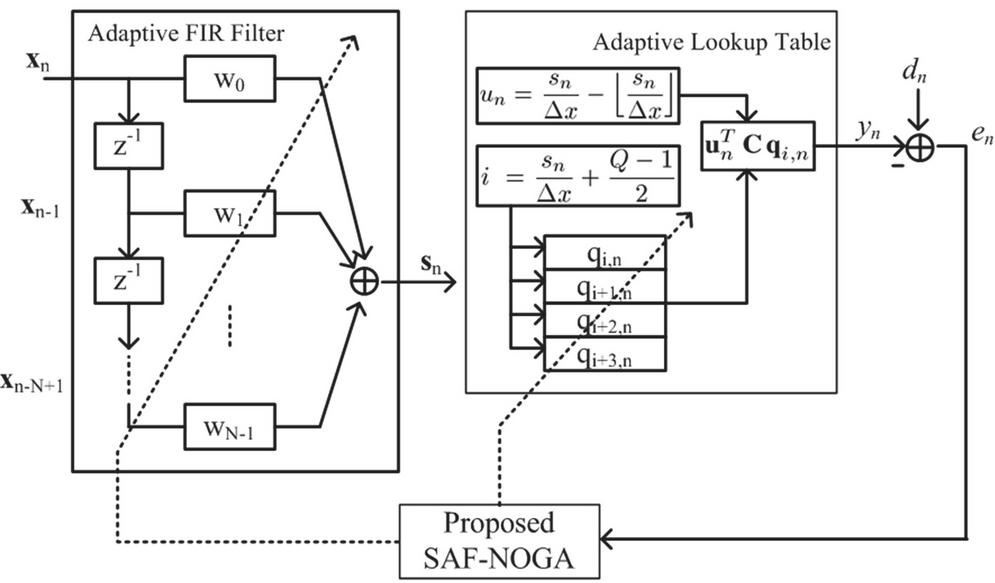
Figure 1 Adaptive tracking of linear-nonlinear network of SAF-NOGA structure.

where $\mathrm{△}x$ is the uniform space between two adjacent control points, and $\mathrm{△}x<0.2977$ [3]. Q is the number of control point. The local parameter vector ${\mathbf{u}}_n$ is defined as ${\mathbf{u}}_n=[u_n^3,u_n^2,u_n,\mathrm{\hspace{0.25em}1}].$

In particular, we obtain the SAF output $y_n$ as [12]

$$y_n={\mathbf{u}}_n^T\mathbf{C}{\mathbf{q}}_{i,n},$$

(3)

where C is the spline basis matrix and ${\mathbf{q}}_{i,n}$ is the control point vector at index i and symbol n.

3 Proposed Spline Adaptive Filtering Normalized Orthogonal Gradient Adaptive Algorithm

Similar to [8], we suppose that the objective function $J({\mathbf{w}}_n,{\mathbf{q}}_{i,n})$ is minimized as

$$J({\mathbf{w}}_n,{\mathbf{q}}_{i,n})=\underset{{\mathbf{w}}_n,{\mathbf{q}}_{i,n}}{min}\left\{\frac{1}{2}({\parallel {\mathbf{w}}_{n+1}-{\mathbf{w}}_n\parallel }^2+{|e_n|}^2)\right\},$$

(4)

where $e_n$ is a priori error given by

$$e_n=d_n-y_n=d_n-{\mathbf{u}}_n^T\mathbf{C}{\mathbf{q}}_{i,n},$$

(5)

where $d_n$ is the desired signal and $y_n$ is the SAF output.

Hence, the minimum value can be obtained by differentiating Equation (4) with respect to ${\mathbf{w}}_n$ and ${\mathbf{q}}_{i,n}$ using the method of chain rule [13, 14] as follows:

${\displaystyle \frac{\partial J({\mathbf{w}}_n,{\mathbf{q}}_{i,n})}{\partial {\mathbf{w}}_n}}$	$=-e_n\left({\displaystyle \frac{\partial y_n}{\partial {\mathbf{u}}_n}}{\displaystyle \frac{\partial {\mathbf{u}}_n}{\partial {\mathbf{s}}_n}}{\displaystyle \frac{\partial {\mathbf{s}}_n}{\partial {\mathbf{w}}_n}}\right)=-{\displaystyle \frac{e_n}{\mathrm{△}x}}\left({\mathbf{u}}_n^{\prime }\mathbf{C}{\mathbf{q}}_{i,n}{\mathbf{x}}_n\right),$	(6)
${\displaystyle \frac{\partial J({\mathbf{w}}_n,{\mathbf{q}}_{i,n})}{\partial {\mathbf{q}}_{i,n}}}$	$=-e_n\left({\displaystyle \frac{\partial y_n}{\partial {\mathbf{u}}_n}}{\displaystyle \frac{\partial {\mathbf{u}}_n}{\partial {\mathbf{s}}_n}}{\displaystyle \frac{\partial {\mathbf{s}}_n}{\partial {\mathbf{q}}_{i,n}}}\right)=-e_n{\mathbf{C}}^T{\mathbf{u}}_n,$	(7)

where ${\mathbf{u}}_n^{\prime }$ is the derivative of ${\mathbf{u}}_n$ as ${\mathbf{u}}_n^{\prime }=[3u_n^2,\mathrm{\hspace{0.25em}2}{u}_n,\mathrm{\hspace{0.25em}1},\mathrm{\hspace{0.25em}0}]$.

Consequently, a recursion of the tap-weight estimated vector ${\mathbf{w}}_n$ toward the minimum based on NOGA algorithm can be written as

$${\mathbf{w}}_{n+1}={\mathbf{w}}_n+{\mu }_w{\mathbf{d}}_{w_n},$$

(8)

where ${\mu }_w$ is the step-size of linear network part of SAF structure and ${\mathbf{d}}_{w_n}$ is the directional vector of tap-weight vector ${\mathbf{w}}_n$ denoted by

$${\mathbf{d}}_{w_{n+1}}={\lambda }_w{\mathbf{d}}_{w_n}-{\mathbf{g}}_{w_n},$$

(9)

where ${\lambda }_w$ is the forgetting-factor of tap-weight vector ${\mathbf{w}}_n$. The negative gradient ${\mathbf{g}}_{w_n}$ of ${\mathbf{w}}_n$ can be evaluated by taking the derivative the cost function in Equation (7) with respect to ${\mathbf{w}}_n$ as

$\therefore {\mathbf{g}}_{w_n}={\lambda }_w{\mathbf{g}}_{w_n}-{\displaystyle \frac{\partial J({\mathbf{w}}_n,{\mathbf{q}}_{i,n})}{\partial {\mathbf{w}}_n}}={\lambda }_w{\mathbf{g}}_{w_n}+\left\{{\displaystyle \frac{e_n}{\mathrm{△}x}}{\mathbf{u}}_n^{\prime }\mathbf{C}{\mathbf{q}}_{i,n}{\mathbf{x}}_n\right\}.$

(10)

According to [10], the forgetting-factor ${\lambda }_w$ of tap-weight vector ${\mathbf{w}}_n$ that places on the orthogonal projection of present gradient vector ${\mathbf{g}}_{w_n}$ and previous directional vector ${\mathbf{d}}_{w_{n-1}}$ is defined as

$${\lambda }_w=\frac{{\mathbf{d}}_{w_{n-1}}^T{\mathbf{g}}_{w_n}}{{\mathbf{d}}_{w_n}^T{\mathbf{d}}_{w_{n-1}}}.$$

(11)

Similarly, the adaptive control point tap-weight vector ${\mathbf{q}}_{i,n}$ is given by

$${\mathbf{q}}_{i,n+1}={\mathbf{q}}_{i,n}+{\mu }_q{\mathbf{d}}_{q_n},$$

(12)

where ${\mathbf{d}}_{q_n}$ is the directional vector of control point vector ${\mathbf{q}}_{i,n}$ in the recursion form as

$${\mathbf{d}}_{q_{n+1}}={\lambda }_q{\mathbf{d}}_{q_n}-{\mathbf{g}}_{q_n},$$

(13)

where ${\lambda }_q$ is the forgetting-factor of ${\mathbf{q}}_{i,n}$.

Since the negative gradient of ${\mathbf{q}}_{i,n}$ can be expressed using the derivation of Equation (7) with respect to ${\mathbf{q}}_{i,n}$ as

$$\therefore {\mathbf{g}}_{q_n}={\lambda }_q{\mathbf{g}}_{q_n}-\frac{\partial J({\mathbf{w}}_n,{\mathbf{q}}_{i,n})}{\partial {\mathbf{q}}_{i,n}}={\lambda }_q{\mathbf{g}}_{q_n}+{\mathbf{u}}_n{\mathbf{C}}^T{e}_n,$$

(14)

where the forgetting-factor ${\lambda }_q$ of tap-weight vector ${\mathbf{q}}_{i,n}$ is computed by

$${\lambda }_q=\frac{{\mathbf{d}}_{q_{n-1}}^T{\mathbf{g}}_{q_n}}{{\mathbf{d}}_{q_n}^T{\mathbf{d}}_{q_{n-1}}}.$$

(15)

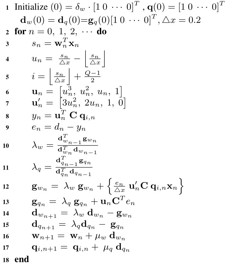
Hence, a proposed SAF based on NOGA algorithm (SAF-NOGA) is described in Algorithm 1.

4 Convergence and Stability Analysis of the Proposed SAF-NOGA Algorithm

Convergence and stability analysis of the proposed SAF-NOGA algorithm are investigated at steady-state as a function of MSE.

4.1 Convergence Analysis

Let us introduce ${\mathbf{w}}_n$ in the approximate form as

${\mathbf{w}}_{n+1}$	$\approx {\mathbf{w}}_n+{\displaystyle \frac{{\mu }_{w_n}{\varphi }_i^{\prime }(u){\mathbf{x}}_n{e}_n}{\mathrm{△}x}},$	(16)
${\varphi }_i^{\prime }(u)$	$={\mathbf{u}}_n^{\prime }\mathbf{C}{\mathbf{q}}_{i,n}.$	(17)

By using the Taylor series expansion, the estimated error $e_n$ is given by

$e_{n+1}$	$\approx e_n+{\displaystyle \frac{\partial e_n}{\partial {\mathbf{w}}_n}}\mathrm{△}{\mathbf{w}}_n,$	(18)
$e_n$	$=d_n-{\varphi }_i^{\prime }(u)=d_n-{\mathbf{u}}_n^T\mathbf{C}{\mathbf{q}}_{i,n}.$	(19)

By differentiating $e_n$ in Equation (19) with respect to ${\mathbf{w}}_n$ using chain rule, we get

$$\frac{\partial e_n}{\partial {\mathbf{w}}_n}=-\frac{\partial {\varphi }_i(u)}{\partial u_n}\frac{\partial u_n}{\partial {\mathbf{s}}_n}\frac{\partial {\mathbf{s}}_n}{\partial {\mathbf{w}}_n}=\frac{{\varphi }_i^{\prime }(u){\mathbf{x}}_n}{\mathrm{△}x}.$$

(20)

---

Algorithm 1 Proposed SAF-NOGA algorithm

---

---

From Equation (16), we rewrite as

$\mathrm{△}{\mathbf{w}}_n={\mathbf{w}}_{n+1}-{\mathbf{w}}_n\approx {\displaystyle \frac{{\mu }_{w_n}{\varphi }_i^{\prime }(u){\mathbf{x}}_n{e}_n}{\mathrm{△}x}}.$

(21)

Substituting Equations (20) and (21) in Equation (18), we then obtain

$\therefore e_{n+1}$	$=e_n-\left({\displaystyle \frac{{\varphi }_i^{\prime }\left(u\right){\mathbf{x}}_n}{\mathrm{△}x}}\right)\cdot \left({\displaystyle \frac{{\mu }_{w_n}{\varphi }_i^{\prime }\left(u\right){\mathbf{x}}_n{e}_n}{\mathrm{△}x}}\right)$
	$=\left\{1-{\displaystyle \frac{{\mu }_{w_n}{\left({\varphi }_i^{\prime }\left(u\right)\right)}^2{\parallel {\mathbf{x}}_n\parallel }^2}{{\left(\mathrm{△}x\right)}^2}}\right\}{e}_n.$	(22)

The norm of both sides of Equation (22) is found as

$\left|e_{n+1}\right|=\left|1-{\displaystyle \frac{{\mu }_{w_n}{\left({\varphi }_i^{\prime }\left(u\right)\right)}^2{\parallel {\mathbf{x}}_n\parallel }^2}{{\left(\mathrm{△}x\right)}^2}}\right|\cdot |e_n|.$

(23)

Therefore, the learning rate of ${\mu }_{w_n}$ in Equation (23) becomes

$\therefore {\mu }_{w_n}={\displaystyle \frac{2{\left(\mathrm{△}x\right)}^2}{{\left({\varphi }_i^{\prime }\left(u\right)\right)}^2{\parallel {\mathbf{x}}_n\parallel }^2}}.$

(24)

Let us consider ${\mathbf{q}}_{i,n}$ in the approximate form as

$${\mathbf{q}}_{i,n+1}={\mathbf{q}}_{i,n}+{\mu }_q{\mathbf{u}}_n{\mathbf{C}}^T{e}_n.$$

(25)

In a similar fashion, the error $e_{n+1}$ can be evaluated as

$e_{n+1}$	$\approx e_n+{\displaystyle \frac{\partial e_n}{\partial {\mathbf{q}}_{i,n}}}\mathrm{△}{\mathbf{q}}_{i,n},$	(26)
$e_n$	$=d_n-{\mathbf{u}}_n^T\mathbf{C}{\mathbf{q}}_{i,n}.$	(27)

By differentiating $e_n$ in Equation (27) with respect to ${\mathbf{q}}_{i,n}$ using chain rule, we obtain

$$\frac{\partial e_n}{\partial {\mathbf{q}}_{i,n}}=-{\mathbf{u}}_n^T\mathbf{C}.$$

(28)

Hence, we rewrite Equation (25) in forms of $\mathrm{△}{\mathbf{q}}_{i,n}$ as

$$\mathrm{△}{\mathbf{q}}_{i,n}={\mathbf{q}}_{i,n+1}-{\mathbf{q}}_{i,n}=-{\mu }_{q_n}{\mathbf{u}}_n{\mathbf{C}}^T{e}_n.$$

(29)

Substituting Equations (28) and (29) into Equation (26), we get

$$\therefore e_{n+1}=e_n+\left({\mathbf{u}}_n^T\mathbf{C}\right)\cdot \left({\mu }_{q_n}{\mathbf{u}}_n{\mathbf{C}}^T{e}_n\right)=\left\{1-{\mu }_{q_n}{\parallel {\mathbf{u}}_n{\mathbf{C}}^T\parallel }^2\right\}{e}_n.$$

(30)

The norm on both sides of Equation (30) is now

$$\left|e_{n+1}\right|\le \left|1-{\mu }_{q_n}{\parallel {\mathbf{u}}_n{\mathbf{C}}^T\parallel }^2\right|\cdot \left|e_n\right|,$$

(31)

and the learning rate of ${\mu }_{q_n}$ is

$$\therefore {\mu }_{q_n}=\frac{2}{{\parallel {\mathbf{u}}_n{\mathbf{C}}^T\parallel }^2}.$$

(32)

4.2 Stability Analysis

Considering the case of linear FIR filter, we define the weight error vector ${\mathit{\eta }}_{w,n}$ as

$${\mathit{\eta }}_{w,n}={\mathbf{w}}_{\mathrm{opt}}-{\mathbf{w}}_n,$$

(33)

where ${\mathbf{w}}_{\mathrm{opt}}$ is the optimal solution shown in Figure 2.

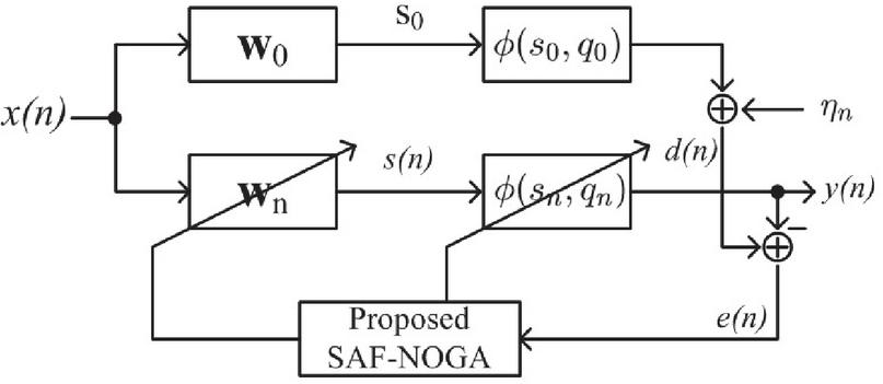
Figure 2 Statistical performance evaluation.

From Equations (16) and (33), we get

$${\mathit{\eta }}_{w,n+1}={\mathit{\eta }}_{w,n}-\frac{{\mu }_{w_n}{\varphi }_i^{\prime }\left(u\right){\mathbf{x}}_n{e}_n}{\mathrm{△}x}.$$

(34)

In this mathematical analysis, we suppose that proposed algorithm has converged under a few assumptions as follows.

Assumption 1: We deliberate the necessary condition for the convergence, in such a way that

$$E\{\parallel {\mathit{\eta }}_{w,n}\parallel \}\to 0,\mathrm{as}n\to \mathrm{\infty }$$

or, equivalently,

$$E\{{\mathbf{w}}_n\}\to {\mathbf{w}}_{\mathrm{opt}},\mathrm{as}n\to \mathrm{\infty }.$$

From Equation (19), we organize the error $e_{w,n}$ in forms of ${\mathbf{w}}_n$ as

$e_{w,n}$	$=d_n-{\mathbf{u}}_n^T\mathbf{C}{\mathbf{q}}_{i,n}$
	$=d_n-{\mathbf{w}}_n^T{\mathbf{x}}_n\mathbf{C}{\mathbf{q}}_{i,n}$
	$=d_n-{\left({\mathbf{w}}_{\mathrm{opt}}-{\mathit{\eta }}_{w,n}\right)}_n^T{\mathbf{x}}_n\mathbf{C}{\mathbf{q}}_{i,n}$
	$=e_{opt,w}+{\mathit{\eta }}_{w,n}^T{\mathbf{x}}_n{\mathbf{Cq}}_{i,n},$	(35)

where $e_{opt,w}$ is an error in the optimal solution in the case of adaptive FIR filter as

$$e_{opt,w}=d_n-{\mathbf{w}}_{\mathrm{opt}}^T{\mathbf{x}}_n{\mathbf{Cq}}_{i,n}.$$

(36)

Let us denote ${𝕁}_{w,n}$ as the expectation of MSE by taking expectation in Equation (35). It can be stated in the form of

${𝕁}_{w,n}$	$=E\left\{{\left|e_{w,n}\right|}^2\right\}$
	$=E\left\{{\left|e_{\mathrm{opt},w}+{\mathit{\eta }}_{w,n}^T{\mathbf{x}}_n\mathbf{C}{\mathbf{q}}_{i,n}\right|}^2\right\}$
	$=E\left\{{\left|e_{\mathrm{opt},w}\right|}^2\right\}+E\left\{\left|e_{\mathrm{opt},w}{\mathit{\eta }}_{w,n}^T{\mathbf{x}}_n\mathbf{C}{\mathbf{q}}_{i,n}\right|\right\}$
	$\mathrm{\hspace{1em}}+E\left\{\left|e_{\mathrm{opt},w}{\mathit{\eta }}_{w,n}{\mathbf{x}}_n^T\mathbf{C}{\mathbf{q}}_{i,n}\right|\right\}+E\left\{{\left|{\mathit{\eta }}_{w,n}^T{\mathbf{x}}_n\mathbf{C}{\mathbf{q}}_{i,n}\right|}^2\right\}.$	(37)

By using Assumption 1, we assume that

$$\therefore {𝕁}_{w,n}={𝕁}_{w,n}^{\min }+{𝕁}_{w,n}^{\mathrm{ex}},$$

(38)

where ${𝕁}_{w,n}^{\min }$ is the minimum mean square error (MMSE) produced by the optimal solution as

$\therefore {𝕁}_{w,n}^{\min }$	$=E\left\{{\left|e_{\mathrm{opt},w}\right|}^2\right\}+E\left\{\left|e_{\mathrm{opt},w}{\mathit{\eta }}_{w,n}^T{\mathbf{x}}_n\mathbf{C}{\mathbf{q}}_{i,n}\right|\right\}$
	$\mathrm{\hspace{1em}}+E\left\{\left|e_{\mathrm{opt},w}{\mathit{\eta }}_{w,n}{\mathbf{x}}_n^T\mathbf{C}{\mathbf{q}}_{i,n}\right|\right\}$	(39)

and ${𝕁}_{w,n}^{\mathrm{ex}}$ is the excess mean square error (EMSE) as

$$\therefore {𝕁}_{w,n}^{\mathrm{ex}}=E\left\{{\left|{\mathit{\eta }}_{w,n}^T{\mathbf{x}}_n\mathbf{C}{\mathbf{q}}_{i,n}\right|}^2\right\}.$$

(40)

Similarly, the weight error vector ${\mathit{\eta }}_{q,n}$ following the case of control points ${\mathbf{q}}_{i,n}$ as

$${\mathit{\eta }}_{q,n}={\mathbf{q}}_{\mathrm{opt}}-{\mathbf{q}}_{i,n},$$

(41)

where ${\mathbf{q}}_{\mathrm{opt}}$ is the optimal solution of control points.

From Equations (25) and (41), we get

$${\mathit{\eta }}_{q,n+1}={\mathit{\eta }}_{q,n}+{\mu }_q{\mathbf{u}}_n{\mathbf{C}}^T{e}_n.$$

(42)

Assumption 2: We deliberate the necessary condition for the convergence, that is,

$$E\left\{\parallel {\mathit{\eta }}_{q,n}\parallel \right\}\to 0,\mathrm{as}n\to \mathrm{\infty }$$

or, equivalently,

$$E\left\{{\mathbf{q}}_n\right\}\to {\mathbf{q}}_{\mathrm{opt}},\mathrm{as}n\to \mathrm{\infty }.$$

From Equation (19), we organize the error $e_{q,n}$ in forms of ${\mathbf{q}}_n$ as

$e_{q,n}$	$=d_n-{\mathbf{q}}_{i,n}^T{\mathbf{Cu}}_n$
	$=d_n-{\left({\mathbf{q}}_{\mathrm{opt}}-{\mathit{\eta }}_{q,n}\right)}_n^T\mathbf{C}{\mathbf{u}}_n$
	$=e_{opt,q}+{\mathit{\eta }}_{q,n}^T\mathbf{C}{\mathbf{q}}_{i,n},$	(43)

where $e_{opt,q}$, the error produced in the optimal solution in the case of control points, is denoted as

$e_{opt,q}=d_n-{\mathbf{q}}_{opt}^T{\mathbf{Cu}}_n.$

(44)

Let us define ${𝕁}_{q_n}$ as the expectation of MSE. It can be given by taking expectation operator on Equation (44) as

${𝕁}_{q,n}$	$=E\left\{{\left|e_{q,n}\right|}^2\right\}$
	$=E\left\{{\left|e_{\mathrm{opt},q}+{\mathit{\eta }}_{q,n}^T{\mathbf{x}}_n{\mathbf{Cu}}_n\right|}^2\right\}$
	$=E\left\{{\left|e_{\mathrm{opt},q}\right|}^2\right\}+E\left\{\left|e_{\mathrm{opt},q}{\mathit{\eta }}_{q,n}^T\mathbf{C}{\mathbf{u}}_n\right|\right\}$
	$+E\left\{\left|e_{\mathrm{opt},q}{\mathit{\eta }}_{q,n}{\mathbf{Cu}}_n\right|\right\}+E\left\{{\left|{\mathit{\eta }}_{q,n}^T{\mathbf{Cu}}_n\right|}^2\right\}.$	(45)

By using Assumption 2, we assume that

$$\therefore {𝕁}_{q,n}={𝕁}_{q,n}^{\min }+{𝕁}_{q,n}^{\mathrm{ex}},$$

(46)

where ${𝕁}_{q,n}^{\min }$ is the MMSE produced by the optimal solution as

$\therefore {𝕁}_{q,n}^{\min }$	$=E\left\{{\left|e_{\mathrm{opt},q}\right|}^2\right\}+E\left\{\left|e_{\mathrm{opt},q}{\mathit{\eta }}_{q,n}^T\mathbf{C}{\mathbf{u}}_n\right|\right\}$
	$\mathrm{\hspace{1em}}+E\left\{\left|e_{\mathrm{opt},q}{\mathit{\eta }}_{q,n}{\mathbf{C}}^T{\mathbf{u}}_n\right|\right\}$	(47)

and ${𝕁}_{w,n}^{\mathrm{ex}}$ is the EMSE as

$$\therefore {𝕁}_{q,n}^{\mathrm{ex}}=E\left\{{\left|{\mathit{\eta }}_{q,n}^T\mathbf{C}{\mathbf{u}}_n\right|}^2\right\}.$$

(48)

5 Simulation Results

For the simulation, the experiments with the random process and an unknown Wiener system constituted by a linear component as shown in [2] are used. A 23-point length LUT ${\mathbf{q}}_0$ is appended to a uniform spline with an interval sampling $\mathrm{△}x=0.2$ [8] as

${\mathbf{q}}_0$	$=\{-2.2,-2,-1.8,\mathrm{\cdots },-1.0,-0.8,-0.91,\mathrm{\hspace{0.25em}0.42},$
	$\mathrm{\hspace{1em}}-0.01,-0.1,\mathrm{\hspace{0.25em}0.1},-0.15,\mathrm{\hspace{0.25em}0.58},\mathrm{\hspace{0.25em}1.2},\mathrm{\hspace{0.25em}1.0},\mathrm{\hspace{0.25em}1.2},\mathrm{\cdots },2.0,\mathrm{\hspace{0.25em}2.2}\}.$

The spline basis matrix, ${\mathbf{C}}_B$ called B-spline and ${\mathbf{C}}_{CR}$ named Catmull-Rom spline are used as follows [2]:

$${\mathbf{C}}_B=\frac{1}{6}\left[\begin{array}{cccc}\hfill -1\mathit{\hspace{1em}}& \hfill 3\mathit{\hspace{1em}}& \hfill -3\mathit{\hspace{1em}}& \hfill 1\\ \hfill 3\mathit{\hspace{1em}}& \hfill -6\mathit{\hspace{1em}}& \hfill 3\mathit{\hspace{1em}}& \hfill 0\\ \hfill -1\mathit{\hspace{1em}}& \hfill 0\mathit{\hspace{1em}}& \hfill 3\mathit{\hspace{1em}}& \hfill 0\\ \hfill 1\mathit{\hspace{1em}}& \hfill 4\mathit{\hspace{1em}}& \hfill 1\mathit{\hspace{1em}}& \hfill 0\end{array}\right],$$

(49)

and

$${\mathbf{C}}_{CR}=\frac{1}{2}\left[\begin{array}{cccc}\hfill -1\mathit{\hspace{1em}}& \hfill 3\mathit{\hspace{1em}}& \hfill -3\mathit{\hspace{1em}}& \hfill 1\\ \hfill 2\mathit{\hspace{1em}}& \hfill -5\mathit{\hspace{1em}}& \hfill 4\mathit{\hspace{1em}}& \hfill -1\\ \hfill -1\mathit{\hspace{1em}}& \hfill 0\mathit{\hspace{1em}}& \hfill 1\mathit{\hspace{1em}}& \hfill 0\\ \hfill 0\mathit{\hspace{1em}}& \hfill 2\mathit{\hspace{1em}}& \hfill 0\mathit{\hspace{1em}}& \hfill 0\end{array}\right].$$

(50)

The comparison of performance of proposed SAF-NOGA (Spline adaptive filter based on normalized orthogonal gradient adaptive algorithm) in accordance with the SAF-LMS (Spline adaptive filter based on least mean square algorithm) [2] in the Wiener system identification over 300 Monte Carlo trials and 10,000 samples is experimented. The generated input signal is the colored signal by [4]

$$x_n=\alpha \cdot x_{n-1}+\sqrt{1-{\alpha }^2}{\zeta }_n,$$

(51)

where ${\zeta }_n$ is a zero mean white Gaussian noise with unitary variance and $\alpha =[0,\mathrm{\hspace{0.25em}0.99}]$.

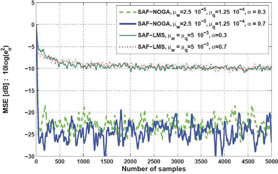
Figure 3 MSE curves of the proposed SAF-NOGA and SAF-LMS [2] using $x_n=\alpha \cdot x_{n-1}+\sqrt{1-{\alpha }^2}{\zeta }_n$, ${\mathbf{C}}_{CR}$ in Equation (50) and SNR $=$ 10 dB.

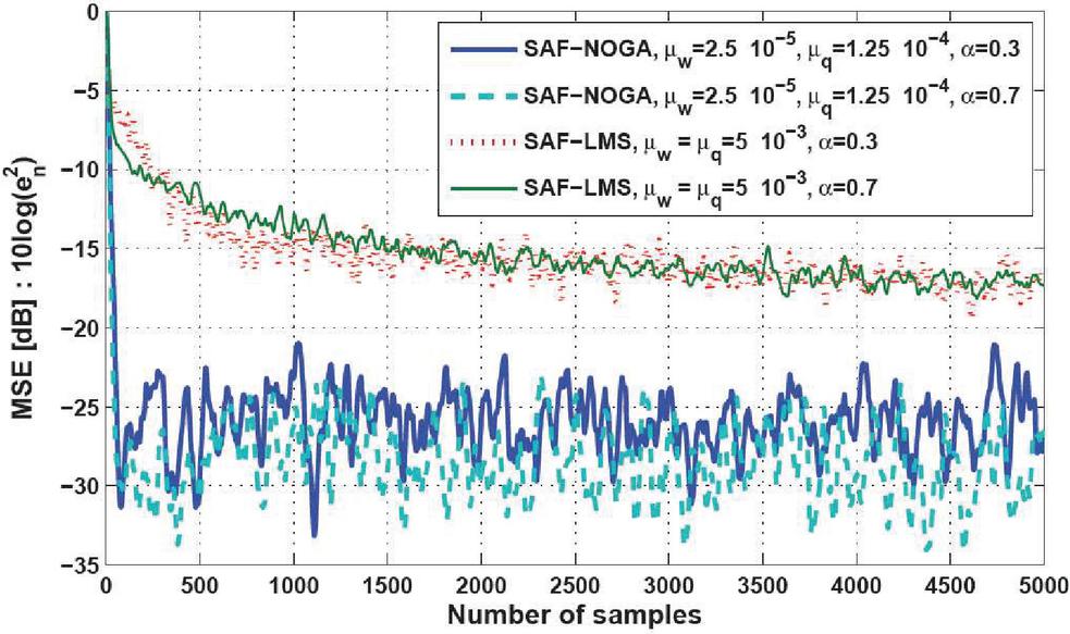
Figure 4 MSE curves of the proposed SAF-NOGA and SAF-LMS [2] using $x_n=\alpha \cdot x_{n-1}+\sqrt{1-{\alpha }^2}{\zeta }_n$, ${\mathbf{C}}_{CR}$ in Equation (50) and SNR $=$ 20 dB.

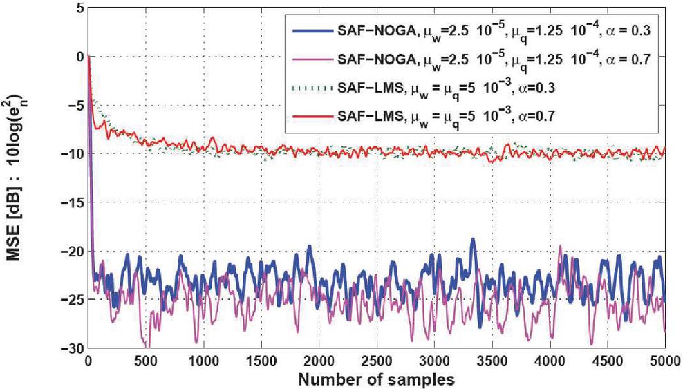
Figure 5 MSE curves of the proposed SAF-NOGA and SAF-LMS [2] using $x_n=\alpha \cdot x_{n-1}+\sqrt{1-{\alpha }^2}{\zeta }_n$, ${\mathbf{C}}_B$ in Equation (49) and SNR $=$ 10 dB.

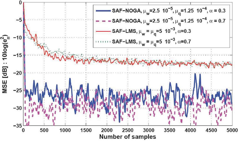
Figure 6 MSE curves of the proposed SAF-NOGA and SAF-LMS [2] using $x_n=\alpha \cdot x_{n-1}+\sqrt{1-{\alpha }^2}{\zeta }_n$, ${\mathbf{C}}_B$ in Equation (49) and SNR $=$ 20 dB.

For SAF model, the initial parameters of adaptive linear FIR filter are as ${\delta }_w=1\times {10}^{-3}$, a signal-to-noise ratio SNR $=$ 10, 20 dB and the length of coefficients M is tantamount to 5 taps. Initial parameters of proposed SAF-NOGA algorithm are determined as follows: ${\mu }_w=2.5\times {10}^{-5},{\mu }_q=1.25\times {10}^{-4},{\lambda }_w=7.5\times {10}^{-4},{\lambda }_q=2.5\times {10}^{-4}$, and of SAF-LMS are as ${\mu }_w={\mu }_q=0.008$.

Comparison of MSE learning curves is used in the simulation with the different values of $\alpha =0.3,\mathrm{\hspace{0.25em}0.7}$. Figures 3 and 4 depict the MSE learning curves of proposed SAF-NOGA and SAF-LMS with these parameters ${\mathbf{C}}_{CR}$ in Equation (50) and SNR $=$ 10, 20 dB, respectively, where the MSE in dB is $10\log (e_n^2)$. It is noted that the MSE learning curves of the proposed SAF-NOGA algorithm rapidly reach the steady-state compared with conventional SAF-LMS algorithm.

In addition, Figures 5 and 6 illustrate the MSE learning curves of proposed SAF-NOGA and SAF-LMS with the parameter ${\mathbf{C}}_B$ in Equation (49) and SNR $=$ 10, 20 dB, respectively. It is mentioned that the MSE learning rate of proposed SAF-NOGA algorithms exhibit a much faster convergence rate.

6 Conclusion

In this paper, the proposed SAF-NOGA algorithm is explained briefly as to how the NOGA algorithm based on the SAF is investigated using the MMSE criterion. The tap-weight estimated vectors of the adaptive FIR filter and control points have been explicated and analyzed for the NOGA algorithm. Convergence and stability analysis of the proposed algorithms have been considered with the excess MSE approach. Performance of the proposed algorithm in terms of MSE and convergence rate to steady-state is revealed. Simulation results show that the MSE learning curves of proposed SAF-NOGA algorithm can enhance the system performance when compared with the SAF-LMS algorithm or the conventional adaptive filters in the real-time dynamic system. This study is expectedly used for applications such as echo cancelation and adaptive filtering in smart communication technology.

References

[1] L. Ljung. System Identification- Theory for the user. Upper Saddle River, NJ. 1999.

[2] M. Scarpiniti, D. Comminiello, R. Parisi and A. Uncini. Nonlinear Spline Adaptive Filtering. Signal Processing, 93(4): 772–783, 2013.

[3] M. Scarpiniti, D. Comminiello, R. Parisi and A. Uncini. Novel Cascade Spline Architectures for the Identification of Nonlinear Systems. IEEE Transactions on Circuits and Systems I: Regular Papers, 62(7): 1825–1835, 2015.

[4] M. Scarpiniti, D. Comminiello, R. Parisi and A. Uncini. Hammerstein Uniform Cubic Spline Adaptive Filtering: Learning and Convergence Properties. Signal Processing, 100: 112–123, 2014.

[5] M. Scarpiniti, D. Comminiello, R. Parisi and A. Uncini. Spline Adaptive Filters: Theory and Applications, Adaptive Learning Methods for Nonlinear System Modeling, ELSEVIER, 47–69, 2018.

[6] S. Guan and Z. Li. Normalised Spline Adaptive Filtering Algorithm for Nonlinear System Identification. Neural Processing Letter, 46(2), 595–607, 2017.

[7] M. Scarpiniti, D. Comminiello, R. Parisi and A. Uncini. Nonlinear System Identification using IIR Spline Adaptive Filters. Signal Processing, 108, 30–35, 2015.

[8] C. Liu and Z. Zhang. Set-membership Normalised Least M-estimate Spline Adaptive Filtering Algorithm in Impulsive Noise. Electronics Letters, 54(6), 393–395, 2018.

[9] P.S.R. Diniz. Adaptive Filtering: Algorithms and Practical Implementation. Springer, 2008.

[10] S. Sitjongsataporn. Convergence Analysis of Greedy Normalised Orthogonal Gradient Adaptive Algorithm. In Proceedings of IEEE International Symposium on Communications and Information Technologies, Bangkok, Thailand, pp. 345–348, 2018.

[11] S. Guarnieri, F. Piazza and A. Uncini. Multilayer Feedforward Networks with Adaptive Spline Activation Function. IEEE Transactions on Neural Network, 10(3): 672–683, 1999.

[12] S. Kalluri, G.R. Arce. General Class of Nonlinear Normalized Adaptive Filtering Algorithms. IEEE Transactions on Signal Processing, 48(8): 2262–2272, 1999.

[13] S. Sitjongsataporn and T. Wiangtong. Spline Adaptive Filtering based on Normalised Orthogonal Gradient Adaptive Algorithm. In Proceedings of IEEE International Conference on Engineering, Applied Sciences and Technology, pp. 575–578, 2019.

[14] S. Prongnuch and S. Sitjongsataporn. Performance Analysis and Enhancement of Spline Adaptive Filtering based on Adaptive Step-size Variable Leaky Least Mean Square Algorithm. Advances in Science, Technology and Engineering Systems Journal, 5(6): 642–651, 2020.

Biographies

Theerayod Wiangtong received the B.Eng. degree (First-class honors) in electronic engineering from King Mongkut’s Institute of Technology Ladkrabang, the M.Sc. degree in satellite communication from University of Surrey, and the PhD. degree in digital system design, co-design from Imperial College, London, UK. Currently, he is an Assistant Professor with the Department of Electrical Engineering, King Mongkut’s Institute of Technology Ladkrabang. His research interests include digital IC design, hardware/software co-design, embedded systems, algorithm and optimization, and data processing.

Suchada Sitjongsataporn received the B.Eng. (First-class honors) and D.Eng. degrees in electronic engineering from Mahanakorn University of Technology, Bangkok, Thailand, in 2002 and 2009, respectively. She has been working as a Lecturer with the Department of Electronic Engineering, Mahanakorn University of Technology since 2002. Currently, she is an Associate Professor with the Department of Electronic Engineering and the Associate Dean for Research at Faculty of Engineering and Technology in Mahanakorn University of Technology. Her research interests are mathematical and statistical models in the area of adaptive signal processing for communications, networking, embedded system, image and video processing, and embedded systems.

Journal of Mobile Multimedia, Vol. 17_4, 657–672.
doi: 10.13052/jmm1550-4646.1748
© 2021 River Publishers

Abstract

1 Introduction

2 Spline Adaptive Filtering

3 Proposed Spline Adaptive Filtering Normalized Orthogonal Gradient Adaptive Algorithm

4 Convergence and Stability Analysis of the Proposed SAF-NOGA Algorithm

4.1 Convergence Analysis

4.2 Stability Analysis

5 Simulation Results

6 Conclusion

References

Biographies