A MultiStack Parallel (MSP) Partition Algorithm Applied to Sorting

Apisit Rattanatranurak and Surin Kittitornkun*

Dept. of Computer Engineering, Faculty of Engineering, King Mongkut’s Institute of Technology Ladkrabang, Bangkok, Thailand 10520

E-mail: apisit.ra@ssru.ac.th; surin.ki@kmitl.ac.th

* Corresponding Author

Received 19 May 2020; Accepted 24 June 2020; Publication 08 September 2020

Abstract

The CPUs of smartphones are becoming multicore with huge RAM and storage to support a variety of multimedia applications in the near future. A MultiStack Parallel (MSP) sorting algorithm is proposed and named MSPSort to support manycore systems. It can be regarded as many threads of single-pivot interleaving block-based Hoare’s algorithm. Each thread performs compare-swap operations between left and right (stacked and interleaved) data blocks. A number of multithreading features of OpenMP and our own optimization strategies have been utilized. To simulate those smartphones, MSPSort is fine tuned and tested on four Linux systems, e.g. Intel i7-2600, Xeon X5670, AMD R7-1700 and R9-2920. Their memory configurations can be classified as either uniform or non-uniform memory access. The statistical results are satisfied compared to parallel-mode sorting algorithms of Standard Template Library, namely Balanced QuickSort and MultiWay MergeSort. Moreover, MSPSort looks promising to be developed further to improve both run time and stability.

Keywords: Partition, Sort, Multithread, Parallel, OpenMP, Stack.

1 Introduction

Manycore CPUs are prevalent in both servers and high-end desktop personal computers as uniform/non-uniform memory access (UMA/NUMA) systems. In the near future, smartphones’ CPUs are becoming multicore towards manycore to support a variety of multimedia applications. Therefore, basic computing algorithms shall be adapted to exploit that. Sorting and data partitioning are mostly based on the well known single-pivot Hoare’s algorithm. It is known as QuickSort divide and conquer (D&Q) behavior. The first level partition is the bottleneck of D&Q Hoare’s algorithm This paper intends to tackle this problem with multithreading techniques while minimizing the unnecessary memory accesses.

In this paper, we propose a single-pivot block-based data partition algorithm named MultiStack Parallel Partition (MSPPartition). As an application of MSPPartition, MSPSort is proposed to recursively divide the data array into shorter subarrays and to sort them in parallel. Unlike other block-based partitioning algorithms, MSPSort is based on stacks rather than queues and deques. Our contributions can be listed here. Firstly, the MSPSort is in-place and requires zero extra memory to buffer the partitioned data. Secondly, the parallel multistack compare-swap operation is similar to the sequential Hoare’s algorithm thus demanding low memory bandwidth. Thirdly, a hybrid breadth-first depth-first task scheduling is proposed to support cache locality while maximizing parallelism.

This paper is organized as follows. Section 2 reviews related background and previous work of parallel D&Q sorting algorithms. The MSPPartition and MSPSort are elaborated in Section 3. Later on, experiment results are discussed in detail. The last section is Conclusions and Furture Work.

2 Background and Related Work

This section consists of the following subsections, Parallel Sorting Algorithms and STLSort: Sequential and Parallel Modes.

2.1 Parallel D&Q Sorting Algorithms

In 1990, Heidelberger et al. [4] first presented simulation results of parallel QuickSort based on three parallel partitioning algorithms using Fetch-and-Add (F&A) operations and two scheduling algorithms. Speedup of 400× can be obtained from sorting 2²⁰ data with upto 500 processors, low-cost F&A operations and other ideal assumptions. In 2003, Tsigas and Zhang [14] proposed a block-based parallel partitioning QuickSort algorithm. The block size is as small the L1 cache which we consider it as fine-grained parallelism. Its speedup of 11× can be achieved with 32 processors of SUN-T1 architecture. Süß and Leopold [12] presented several alternative algorithms of parallel QuickSort based on Pthread and OpenMP 2.0 in 2004. It can achieve 3.24× on a 4-core AMD Opteron 848. In 2007, Singler et al.[11] developed Multi-Core Standard Template Library (MCSTL) based on C++ Standard Template Library. This parallel sorting algorithm is similar to Tsigas and Zhang’s [14] with a double-ended queue (deque). Its Speedup of 21× can be achieved on an 8-core 32-thread SUN-T1.

In 2008, Traoré et al. [13] described work-optimal parallelizations of STL sort based on work-stealing technique. However, their Introspective sort based on parallel block-based partition [8], [15] is deque-free. Speedup of 8.1× with 16 processors can be obtained. One year later in 2009, Ayguadé et al.[2] proposed MultiSort based on MergeSort which splits the input data equally, sorts them using QuickSort in parallel and then merges them using OpenMP 3.0 Task construct. A maximum Speedup of 13.6× on 32 cores can be achieved with Intel’s C++ Compiler version 9.1 and Cilk compiler version 5.4.3 using last in first out software thread queue. Meanwhile, Man et al. [6, 7] developed psort(), a hybrid QuickSort and MergeSort algorithm. Their work can achieve 11×-Speedup on a 24-core Intel Xeon 7460 system.

In 2013, Mahafzah [5] split the input array with multi-pivot/threads into partitions using extra space and then sort them in parallel with 8 software threads. Speedup of 3.8× is achieved on a dual-core HyperThread processor. Later on, Ranokpanuwat and Kittitornkun [9] proposed Parallel Partition and Merge QuickSort (PPMQSort). They can achieve Speedup of 12.29× relative to qsort() on an 8-core HyperThread Xeon E5520 in 2016. More recently in 2017, Axtmann et al. [1] presented an IPS⁴o sorting algorithm. It is a recursive multithread in-place bucket sort. Each thread is responsible for classifying a number of data blocks into local k buckets based on multipivot values. The local buckets are merged to replace the input array. Once the merged subarrays are shorter and then sorted independently. Speedup can be as high as 29× over its sequential version on a 32-core Intel Xeon E5-2683 v4. In 2018, Rattanatranurak [10] proposed parallel sorting named Dual Parallel Partition sorting (DPPSort). Speedups of 5.95× and 4.70× can be achieved relative to qsort(), and STLSort, respectively on 4-core Hyper-Thread Intel i7-3770. In summary, Table 1 compares some parallel sorting algorithms in chronological order such as partition granularity, bottleneck, recursion, Big-O time complexity and parallel library.

Table 1 Comparison of Sorting Algorithms in terms of Partition Granularity, Merge Algorithm, Time Complexity and Library in chronological order (BQSort: Balanced QuickSort, MWSort: MultiW Merge Sort, DFWSort: Deque-Free Work-Optimal Parallel STLSort, PMQSort: Parallel Multithreaded QuickSort, PPMQSort: Parallel Partition and Merge QuickSort, IPS⁴o: In-Place Parallel Super Scalar Sample Sort, DPPSort: Dual Parallel Partition Sort (B-neck: Bottleneck, Seq: Sequential, NA: Not Available, N: Array Size, c: CPU cores)

Algorithm	[14](2003)	[11](2007)
Name	PQuicksort	BQSort
Granularity	Fine: L1 Cache	Fine: L1 Cache
B-neck	Seq Swap to Middle	Swap to Middle
Recursive	Yes	Yes
Time	$O (\frac{N}{c} \log \frac{N}{c} + \frac{N}{c})$	$O (\frac{N}{c} \log N + c \log c)$
Library	Pthread	OpenMP

Algorithm	[11](2007)	[13](2008)

Name	MWSort	DFWSort
Granularity	NA	Fine: L1 Cache
B-neck	pW merging	Swap to Middle
Recursive	Yes	Yes
Time	$O (\frac{N}{c} \log N + (c \log c) (\log \frac{N}{c}))$	$O (\frac{N}{c} + \log^{3} N)$
Library	OpenMP	OpenMP

Algorithm	[6](2009)	[9](2016)

Name	psort	PPMQSort
Granularity	Coarse: N/c	Coarse: N/2
B-neck	Seq Merge then qsort	Seq Swap
Recursive	No	Yes
Time	$O (\frac{N}{c} \log \frac{N}{c} + N)$	$O (\frac{N}{c} \log \frac{N}{2 c} + N)$
Library	OpenMP	OpenMP

Algorithm	[1](2017)	[10] (2018)

Name	IPS⁴o	DPPSort
Granularity	Fine: block-based	Coarse: N/2
B-neck	In-place buckets	Partition then Swap
Recursive	Yes	Yes
Time	NA	$O (\frac{N}{c} \log \frac{N}{2 c} + N)$
Library	OpenMP	OpenMP

2.2 STLSort: Sequential and Parallel Modes

The Standard Template Library (STL)Sort is a sequential sorting function for any data type. It is available in almost C++ compilers and prototyped as follow.

Parameters first and last are pointers to the first and the last positions, respectively. On the other hand, GNU libstdc++ parallel mode [11] provides two parallel sorting functions based on OpenMP. Namely, Balanced Quick-Sort and Multiway Merge Sort, are subject to evaluation in our experiments. Its function is declared in < parallel/algorithm > directive as follow.

2.2.1 Balanced QuickSort (BQSort)

BQSort is block based similar to Tsigas and Zhang’s [14] partition method. It compares/swaps data between pairs of left and right blocks in parallel until either side is finished. The unfinished (leftover) data blocks are pushed to a double ended queue (deque) to process later. As a result, a pair of blocks can be stolen to any free processor core. The unfinished blocks are swapped to the middle of the input array so that the array can be eventually partitioned. Sequential STLSort is executed locally after it is partitioned successfully. It is claimed to be an in-place algorithm which can be load-balanced using Work Stealing method. Run time of this algorithm is varied depending on data distribution.

2.2.2 MultiW Merge Sort (MWSort)

MWSort divides data into several subarrays equally and STLSort them in parallel. Each subarray is sorted independently with small overheads. MWSort relies on parallel multiway merging algorithm to obtain the final data array. Subsequently, the sorted temporary array is copied to the input array. As a result, this MWSort requires at least twice the space of input data size. Its run time is stable compared with quicksort algorithm.

3 MultiStack Parallel Sort (MSPSort)

This section begins with the overview of our algorithm consisting of the Recursive MultiStack Parallel Partition and Sorting Phases. Consecutively, a number of BF-DF Scheduling algorithms are proposed and compared.

In the MSPSort() function, Median of Five function MO5() (Alg. 1, line 5) selects a pivot index p and moves it to the middle of array A. The Recursive MSPPartition partititions the input array A according to the pivot and finally returns the position of pivot p (Alg. 1, line 7). MSPSort continues according to our proposed scheduling (Alg. 1, lines 12 and 15). The resulting shorter than u_stl subarray is sorted as an independent thread (Task) (Alg. 1, line 20) using STLSort where u_stl = U_stl × κ_l3/sizeof(Type), U_stl is Sorting Cutoff parameter, κ_l3 represents the Level 3 cache size and Type corresponds to the data type to be sorted. Note that, the number of software threads τ is reduced to τ/2 (Alg. 1, line 9) and remained at τ = τ_max/r in order to balance the workload and achieve parallelism where τ_max is the maximum number of threads and r is called Reduction factor.

3.1 Recursive MultiStack Parallel Partition Phase

The Recursive MultiStack Parallel Partition Phase consists of 2 steps: Parallel Stacked Blocks Partition Step and Middle Blocks Partition Step.

The Parallel Stacked Blocks Partition Step begins with dividing A = A[0], A[1], . . . , A[N − 1], an unsorted array into left and right halves. Each half is divided into blocks of b = B × κ_l3/sizeof(Type) elements from both ends (Alg. 2, line 4) where B is a block size parameter. Both left and right block boundaries on the both halves are assigned in round robin to τ threads and pushed from the middle towards both ends (Alg.2, lines 4 and 5). Therefore, each thread is assigned with about the same number of blocks to manipulate and balance the workload while achieving parallelism simultaneously.

When the stacks are ready, OpenMP parallel for is applied to fork τ threads (Alg. 2, line 8) with private (local to each thread) variables i, j, l_b, r_b. Subsequently, these block boundaries are popped off so that data within the left and right blocks can be compared with A[p] and swapped from both ends to the middle until either local left or right stack is empty (Alg. 2, lines 10). Each thread has its own private variables i and j that are left and right indices of the current left and right blocks, respectively. In addition, variables, l_b and r_b are the current boundaries of left and right blocks, respectively. Eventually, the boundaries of the unfinished block are pushed back to their corresponding stacks (Alg.2, lines 27 and 30). This step stops when all τ threads finish.

After that, two indices, l_min = min(L_s[t],∀t) and r_max = max(R_s[t], ∀t) of all τ threads, must be determined to compute r_max − l_min whether the leftover part is longer than u_stl (Alg. 2, line 37). In Middle Blocks Partition Step, the length of the leftover can indicate the number of μ threads to call MSPPartition() (Alg. 2, line 38) just in case. Otherwise, the Lomuto’s Partition [3] eventually returns the pivot index p (Alg. 2, line 41). That is because Lomuto’s algorithm requires fewer memory accesses than Hoare’s.

3.2 Sorting Phase

In the earlier phase, the data subarray is partitioned into smaller subarrays recursively. Any shorter subarray up to u_stl elements can be sorted using STLSort as a independent task (Alg. 1, lines 20 and 42) without any synchronization (OpenMP no wait).

3.3 BF-DF Scheduling Algorithms

The Recursive MSPPartition Phase initially employs default scheduling of OpenMP and thus called BF (Breadth First) method to achieve high parallelism. The problem of BF scheduling is due to its random order of executions depending on the partition sizes and branch/memory stalls. This may cause unnecessary page faults and cache misses. To avoid this problem, we have proposed and implemented DF (Depth First) sorting algorithm in DFMSP-Sort() function. Once enough number of tasks are queued up in the thread pool by BF algorithm, the partitioning process is continued in DF order.

Initially, if the subarray (j_R − i_L) is still greater than u_df elements (Alg. 1, line 11), BFMSPSort() is called recursively (Alg. 1, line 12) as two OpenMP tasks. In other words, BFMSPSort() is executed recursively and continued until the resulting subarray is smaller than u_df elements where u_df = U_df × κ_l3/sizeof(Type) and U_df is Scheduling Cutoff. Otherwise, the alternative DFMSPSort() function is invoked instead (Alg. 1, line 15).

On line 32 of Alg. 1, a local stack P_s is instantiated to keep the subarray boundaries and enforce the execution order so that last-level cache misses can be minimized. Programmers can easily implement the DF scheduling by themselves without worrying about OpenMP supports. It makes use of a local stack P_s to keep the subarray boundaries. This stack can order the execution with one of these scheduling algorithms, RAL, LAL, SPF and LPF, to improve cache locality.

3.3.1 RAL vs. LAL

First of all, the first partition is pushed onto the stack P_s (Alg. 1, line 31). The popped off indices i_L, j_R are passed to Recursive MSPPartition Phase (Alg. 1, line 36). Once the left and right subarrays are obtained, the boundaries of the left one are pushed prior to the right one resulting to depth first traversal to the right hand side (Right Always: RAL). The Recursive MSPP Phase continues until the subarray is shorter than u_stl. Note that STLSort is executed independently with OpenMP nowait compiler directive (Alg. 1, line 43). The traversal continues until P_s is empty (Alg. 1, line 32). The LAL (Left Always) algorithm is the opposite of RAL.

3.3.2 SPF vs. LPF

Both RAL and LAL algorithms make the decisions based on the direction only regardless of the subarray size. It can be more beneficial to our MSPPartition if cache replacement policy is taken into consideration. The shorter partition first (SPF) and longer partition first (LPF) decide longer or shorter subarray to push onto the stack first, respectively. As such, the SPF decision may exploit more recently accessed data inside the caches. On the other hand, the LPF one may prefer longer workload to sustain parallelism.

4 Experiments, Results and Discussions

This section presents how to set up the experiments on four different Linux systems. Experiment parameters are listed and rationalized. Consecutively, the obtained results are elaborated and discussed.

4.1 Experiment Setup

The proposed MSPSort algorithm is evaluated on four different systems as listed in Table 2. They all run the same Ubuntu 18.04 LTS and G++ version 7.4.0. Both Intel and AMD processors are provided equally and subject to our resource constraints. The number of cores c is reported by Linux System Monitor. Moreover, these systems widely differ in terms of memory size, technology and configuration. Nonetheless, their caches are quite similar. Most of their L3 caches are multiples of 8MB that we use κ_ls to denote. Note that NUMA stands for non-uniform memory access time. R7-1700 consists of two memory controllers, one on each die and interconnected with the Infinity Fabric. That results in non-uniform memory latency [www.tomshardware.com].

The experiments are parameterized as shown in Table 3. The data types to be evaluated include Unsigned 32-bit integer (Uint32), Unsigned 64-bit integer (Uint64) and 64-bit double precision floating point numbers (Double). They are randomized with uniform distribution. All algorithms are optimized with -O2 compiler flag. The data size N ranges from 200M to 2000M elements due to system RAM limit. Our proposed BF-DF scheduling can be chosen among these algorithms, LPF, SPF, RAL and LAL.

Table 2 Specifications of multicore CPUs in experiments, KB: Kilobytes, MB: Megabytes

Series Number	Core i7 i7-2600	Xeon X5670	Ryzen R7-1700	ThreadRipper R9-2920
Clock (GHz)	3.40	2.93	3.00	3.50
c (cores)	8	24	16	24
Sockets	1	2	1	1

RAM	32GB	24GB	32GB	64GB
Configuration	4×8GB	12×2GB	4×8GB	8×8GB
Technology	DDR3	DDR3	DDR4	DDR4
NUMA	No	Yes	Almost	Yes
Memory	2 ch	4 ch	2 ch	4 ch

L1 I-Cache	4×32KB 8W	2×6x32KB 4W	8×64KB 4W	12×64KB 4W
L1 D-Cache	4×32KB 8W	2×6x32KB 8W	8×32KB 8W	12×32KB 8W
L2 Cache	4×256KB 8W	2×6x256KB 8W	8×512KB 8W	12×512KB 8W
L3 Cache	8MB 16W	2×12MB 16W	2×8MB 16W	4×8MB 16W

Table 3 Experiment parameters of MSPSort, BF: Bread-First, DF: Depth-First,M=10⁶

Parameters	Values
Algorithms	MSPSort, BQSort, MWSort
Data Types	Uint32, Uint64, Double
Random Dist	Uniform
GCC Optimization	O2
Data size N	200M, 500M, 1000M, 2000M

Scheduling	RAL, LAL, LPF, SPF
L3 Cache size κ_l3	8MB
Block size B(×κ_l3)	10⁻⁴, 10⁻³, 10⁻², 10⁻¹, 1
Cutoff U_stl(×κ_l3)	0.5, 1, 2, 4, 8
Cutoff U_df (×κ_l3)	0.5, 1, 2, 4, 8, 16
Multiplier m	1, 2, 4
Reduction r	c, c/2, c/3, c/4

As mentioned earlier, the block size B, Sorting Cutoff U_stl and Scheduling Cutoff U_df are functions of L3 Cache size κ_l3=8MB. The block size B=10⁻⁴, 0.001, 0.01, 0.1, 1. Sorting Cutoff U_stl = 0.5, 1, 2, 4. Scheduling Cutoff U_df = 1, 2, 4, 8, 16. The Multiplier m is set to be power of two, m = 1, 2, 4 as such the MSPSort can fork as many τ_max = c × m threads. The Reduction r can be formulated as a function of c cores reported by the OS, r = c, c/2, c/3, c/4.

4.2 Key Performance Indicators (KPIs)

In this paper, some experiment results shall be normalized and compared based on these KPIs. They all represent time domain aspects of each sorting algorithm.

4.2.1 Average Run Time (T̄) and Run Time per 100M (T̄_100M)

The Average Run Time (T̄) is averaged over a number of trials as specified in each experiment. The proposed Run Time per 100M (T̄_100M) is easy to visualize and compare at any data size for certain experiments. In addition, this normalized run time can enable comparison between systems.

4.2.2 Standard Deviation of T (σ_T) and T_100M (σ_100M)

Run Time Standard of Deviation (σ_T) represents the stability of each algorithm due to the randomness of generated data set. In addition, the normalized standard deviation (σ_100M) can justify some parameters specially Block size B and U_stl.

4.2.3 Run Time Statistics

In addition to arithmetic mean and standard deviation of of Run Time T, the first, second and third quartiles are T_Q1, T_Q2 and T_Q3, respectively. In addition, InterQuartile Range can be determined as T_IQR=T_Q3-T_Q1 for stability analyses. These statistics can specify how the Run Time T distributes over 1,000 trials.

4.3 Single-Round MSPPartition

This single round MSPPartition is a prerequisite experiment as a guidance to the main ones. In order to fine tune block size B, a simple partition is tested at various block sizes as listed in Table 3. This experiment is intended to investigate Block size B effects of MSPPartition (Alg. 2, Line 1). Within this experiment, data within left and right blocks are always swapped to get rid of branch prediction (comparison) effects, Given a data array size N, Function MSPPartition is executed for just one round without further recursive calls. The Block size B in this experiment spans a wide range, {10⁻⁴, 0.001, 0.01, 0.1, and 1}×κ_l3 cache size. The maximum number of threads τ_max = c × 1. Note that OpenMP nested parallelism flag is turned off, omp_set_nested(0).

The resulting T̄_100M (bar) and ±σ_100M (error bar) in seconds are plotted in Figure 1 at different data sizes after 100 trials. All systems show the same behavior of T̄_100M vs B. It can also be observed that the larger the data size N, the higher the T̄_100M. This can be due to poor cache locality accessing data from both ends. The smallest B=10⁻⁴ × κ_l3 ≈800 Bytes yields the worst performance. The best T̄_100M can be found as B ranges between 0.001 to 0.1 × κ_l3 that is between the size of L1 and L2 caches. As a result, B = 0.01 × κ_l3 is chosen as a representative.

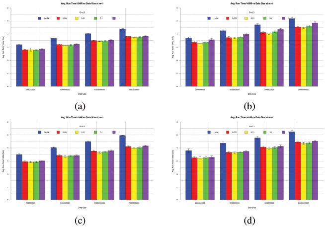
Figure 1 T̄_100M (Bargraph) and ±σ_100M (Error bar) of Single-Round MSPPartition at B={10⁻⁴, 0.001, 0.01, 0.1, 1}×κ_l3, m=1 (a) i7-2600, (b) X5670, (c) R7-1700, (d) R9-2920 for Uint32 data and 100 trials

Note that all graphs are plotted on the same scale of Y axis. With m=1, each system gets different number of threads c to execute. That means i7-2600 can achieve lower T̄_100M on the same N than X5670 despite much lower core count. Similarly, R7-1700 yields faster T̄_100M than R9-2920 despite lower clock frequency and lower core count. This phenomenon could be due to non-uniform (longer) memory access of large data arrays on X5670 and R9-2920 as listed in Table 2.

4.4 Parallel Sorting of Independent Data Blocks

To investigate how Sorting Cutoff U_stl affects the Run Time, a data array of N elements is divided with equal chunks of u_stl elements and assigned to a thread to sort in parallel. Divided subarrays are independently STLsorted with c × 1 threads as m=1. Note that OpenMP nested parallelism flag is turned off just like the previous experiment. This experiment can be beneficial to any D&Q sorting algorithm in general because the partitioning overhead is neglected. The random data array of a given size N is divided equally to U_stl={10⁻⁴, 0.001, 0.01, 0.1, 1}×κ_l3.

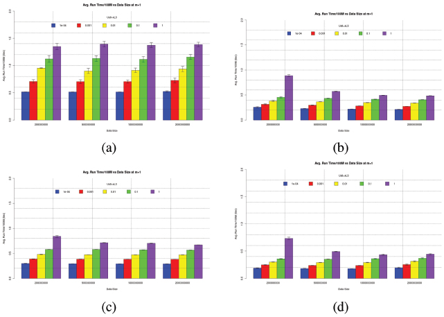
Figure 2 T̄_100M (Bargraph) and ±σ_100M (Error bar) of Independent Parallel Sort at [U_stl={10⁻⁴, 0.001, 0.01, 0.1,1} × κ_l3, m=1 (a) i7-2600, (b) X5670, (c) R7-1700, (d) R9-2920 for Uint32 data and 100 trials

The experiment is repeated for 100 trials to obtain T̄_100M (bar) and σ_100M (error bar) as plotted in Figure 2. In general, the same behavior can be observed for all systems. It can be noticed that given the same data size N the smaller cutoff U_stl the lower T̄_100M. This can be concluded that smaller U_stl is better provided that there is no dependency between these data chunks.

4.5 MSPSort with BF Scheduling

The current and later experiments are different from the preliminary ones where OpenMP Nested Parallelism is switched ON and MSPPartition is recursively invoked. MSPSort with BF scheduling corresponds to line 12 of Alg. 1 and line 11 is always true. Due to an extremely large number of parameter combinations, this experiment is intended to obtain and pick (m, r) pair with the most consistent performance for each system. Run Time T’s are collected according with BF Scheduling for all N’s, B=0.01, U_stl=0.5, 1, 2, 4 after 20 Trials. The (m, r) pairs with most appearances in Top-10 minimum T̄ of all data size N are listed in Table 4. The most consistent (m,r) pairs (top row of each data type) in Table 4 are selected for each system/data type as representatives for the next experiment.

Table 4 Top-three (m,r) pairs with BF Scheduling for all N’s, B=0.01, U_stl=0.5,1,2,4 after 20 Trials

System	i7-2600	X5670	R7-1700	R9-2920
Uint32	(2,8)	(1,6)	(2,16)	(2,12)
	(1,8)	(2,12)	(2,8)	(1,8)
	(2,4)	(1,8)	(1,16)	(1,6)

Uint64	(2,8)	(1,6)	(2,16)	(1,8)
	(1,4)	(2,12)	(1,8)	(1,6)
	(2,4)	(1,8)	(2,8)	(2,12)

Double	(2,8)	(1,6)	(2,16)	(1,8)
	(1,4)	(2,12)	(1,8)	(1,6)
	(2,4)	(1,8)	(2,8)	(2,12)

4.6 MSPSort with BF-DF Scheduling

This experiment is intended to obtain the most consistent performance of (U_stl, U_df) pair and BF-DF scheduling algorithm given each data size N as listed in Table 5 for each system after 100 trials. For all data types, it can be observed that the (m,r) pairs are almost the same on many systems except R9-2920. It is not guaranteed that these parameters can yield consistent performance. Therefore, extensive run time statistics should be collected and compared against BQSort and MWSort.

Table 6 to Table 9 tabulates the run time statistics of all sorting algorithms after 1000 trials. According to the chosen parameters in Table tb:para:chosen, the time-domain KPIs of MSPSort can be investigated analyzed thoroughly. Although lower T̄ and σ_T are better in terms of run time and stability, other statistics play important roles as well. We shall discuss the experiment results with respect to the following aspects.

4.6.1 Sorting vs Scheduling Cutoffs

There are two different approaches of BF-DF scheduling, direction versus size oriented. Both RAL and LAL are direction oriented. On the contrary, LPF and SPF are size oriented. SPF and LPF are good for small data type such as Uint32. It can be also noticed that they mostly are characterized by smaller (U_stl,U_df) pairs. On the other hand, LAL and RAL are beneficial to MSPSort on larger data types such as both Uint64 and Double. The (U_stl,U_df) pairs are generally larger than those of Uint32.

Table 5 Chosen parameters U_stl:U_df:m:r, B=0.01 after 100 trials

System	i7-2600	X5670	R7-1700	R9-2920
Uint32
BFDF	LPF	SPF	SPF	SPF
N=200M	0.5:2:2:8	0.5:1:1:6	0.5:1:2:16	0.5:1:2:12
N=500M	0.5:2:2:8	1:4:1:6	1:2:2:16	1:2:2:12
N=1000M	0.5:2:2:8	1:8:1:6	2:4:2:16	1:4:2:12
N=2000M	4:8:2:8	2:16:1:6	2:4:2:16	2:4:2:12

Uint64
Double
BFDF	RAL	RAL	LAL	LAL
N=200M	1:8:2:8	2:4:1:6	1:2:2:16	0.5:2:1:8
N=500M	1:8:2:8	2:4:1:6	1:2:2:16	1:4:1:8
N=1000M	2:8:2:8	4:8:1:6	2:2:2:16	2:8:1:8
N=2000M	2:8:2:8	4:8:1:6	2:2:2:16	2:8:1:8

As shown in Figures 1 and 2, all systems behave in the same fashion. It can be noticed in Figure 1 that T̄_100M significantly increases as N doubles up for all systems. Unlike partitioning T̄_100M, sorting T̄_100M is almost constant for all data sizes N given the same U_stl. That means sorting can be traded off with partitioning at larger N as the subarrays become shorter.

In order to minimize the Run Time T, BD-DF Cutoff U_df grows according to N to reduce the recursion levels. We have showed in Figure 1 that partitioning T̄_100M is significantly higher as N doubles. Sorting cutoff U_stl is quite similar to U_df. It can be observed that U_stl is proportional to U_df as well. That is because sorting T̄_100M grows slowly as U_stl is ten fold longer in Figure 2. Therefore, sorting a longer subarray can take the same amount of time as partitioning it and sorting two resulting shorter subarrays.

4.6.2 Memory Architecture

Compared to BQSort only, MSPSort can achieve better run time statistics on all data types on every system except X5670. This can be due to the fact that BQSort can steal the workloads to distribute to available CPU cores. Thus, BQSort is more tolerant to multi-socket NUMA effects than MSPSort.

Table 6 Statistics of Run Time T of MSPSort vs BQSort vs MWSort for all data types at various sizes N on i7-2600 system after 1000 trials

Alg.	KPI (Sec.)	200M	500M	1000M	2000M
Uint32
MSPSort	T_Q1	3.042	8.113	17.832	37.880
	T_Q2	3.073	8.179	17.963	38.340
	T̄	3.182	8.342	17.928	38.332
	T_Q3	3.318	8.283	18.039	38.797
	σ_T	0.196	0.436	0.171	0.536

BQSort	T_Q1	3.212	8.578	18.285	38.670
	T_Q2	3.247	8.665	18.447	39.105
	T̄	3.348	8.856	18.484	39.503
	T_Q3	3.491	8.804	18.663	40.130
	σ_T	0.198	0.503	0.270	1.111

MWSort	T_Q1	3.649	9.550	20.132	40.920
	T_Q2	3.700	9.675	20.382	41.588
	T̄	3.812	9.710	20.385	41.764
	T_Q3	4.016	9.812	20.633	42.470
	σ_T	0.231	0.266	0.383	1.105

Uint64
MSPSort	T_Q1	3.648	9.855	21.540	44.592
	T_Q2	3.772	9.909	21.725	44.813
	T̄	3.813	9.956	21.712	44.887
	T_Q3	4.065	9.973	21.893	45.104
	σ_T	0.205	0.234	0.243	0.454

BQSort	T_Q1	3.702	10.023	21.780	45.898
	T_Q2	3.767	10.104	21.976	46.332
	T̄	3.877	10.254	21.977	46.511
	T_Q3	4.151	10.233	22.144	47.073
	σ_T	0.227	0.442	0.270	0.776

MWSort	T_Q1	4.194	11.202	23.721	49.292
	T_Q2	4.253	11.312	23.947	49.633
	T̄	4.326	11.338	23.975	49.703
	T_Q3	4.360	11.449	24.218	50.044
	σ_T	0.209	0.233	0.391	0.709

Double
MSPSort	T_Q1	3.851	10.521	22.908	48.058
	T_Q2	3.917	10.595	23.048	48.684
	T̄	4.013	10.725	23.050	49.038
	T_Q3	4.110	10.693	23.187	50.166
	σ_T	0.222	0.422	0.202	1.151

BQSort	T_Q1	3.937	10.754	23.399	49.553
	T_Q2	4.093	10.962	23.711	50.771
	T̄	4.197	11.235	23.769	50.883
	T_Q3	4.413	11.283	24.183	52.384
	σ_T	0.266	0.706	0.458	1.484

MWSort	T_Q1	4.247	11.361	24.243	50.250
	T_Q2	4.522	11.873	25.080	51.807
	T̄	4.522	11.857	25.122	52.190
	T_Q3	4.696	12.213	25.966	54.108
	σ_T	0.312	0.607	0.939	2.212

Table 7 Statistics of Run Time T of MSPSort vs BQSort vs MWSort for all data types at various sizes N on R7-1700 system after 1000 trials

Alg.	KPI (Sec.)	200M	500M	1000M	2000M
Uint32
MSPSort	T_Q1	1.722	4.416	9.382	19.238
	T_Q2	1.735	4.438	9.413	19.294
	T̄	1.746	4.476	9.418	19.307
	T_Q3	1.773	4.561	9.445	19.353
	σ_T	0.032	0.083	0.063	0.120

BQSort	T_Q1	1.780	4.643	9.897	20.358
	T_Q2	1.811	4.722	10.051	20.695
	T̄	1.807	4.725	10.026	20.635
	T_Q3	1.827	4.778	10.125	20.845
	σ_T	0.032	0.101	0.160	0.316

MWSort	T_Q1	1.973	5.096	10.436	21.290
	T_Q2	2.145	5.470	11.114	22.498
	T̄	2.109	5.389	10.959	22.214
	T_Q3	2.187	5.549	11.241	22.696
	σ_T	0.041	0.086	0.146	0.236

Uint64
MSPSort	T_Q1	2.149	5.723	12.046	25.406
	T_Q2	2.161	5.744	12.091	25.494
	T̄	2.163	5.752	12.104	25.514
	T_Q3	2.174	5.772	12.144	25.584
	σ_T	0.022	0.048	0.092	0.168

BQSort	T_Q1	2.137	5.706	11.990	25.231
	T_Q2	2.153	5.746	12.077	25.423
	T̄	2.160	5.762	12.102	25.487
	T_Q3	2.177	5.805	12.196	25.671
	σ_T	0.033	0.083	0.158	0.348

MWSort	T_Q1	2.216	5.845	12.184	25.469
	T_Q2	2.225	5.864	12.223	25.625
	T̄	2.227	5.868	12.228	26.223
	T_Q3	2.236	5.887	12.268	27.148
	σ_T	0.015	0.033	0.063	0.890

Double
MSPSort	T_Q1	2.312	6.094	12.699	26.616
	T_Q2	2.324	6.120	12.749	26.720
	T̄	2.327	6.125	12.757	26.745
	T_Q3	2.338	6.146	12.805	26.829
	σ_T	0.026	0.046	0.090	0.210

BQSort	T_Q1	2.312	6.097	12.721	26.568
	T_Q2	2.327	6.134	12.799	26.751
	T̄	2.333	6.147	12.830	26.810
	T_Q3	2.347	6.188	12.906	26.942
	σ_T	0.030	0.074	0.159	0.631

MWSort	T_Q1	2.735	7.037	14.366	29.394
	T_Q2	2.774	7.106	14.485	29.608
	T̄	2.778	7.121	14.505	29.628
	T_Q3	2.818	7.196	14.626	29.838
	σ_T	0.051	0.120	0.191	0.333

Table 8 Statistics of Run Time T of MSPSort vs BQSort vs MWSort for all data types at various sizes N on X5670 system after 1000 trials

Alg.	KPI (Sec.)	200M	500M	1000M	2000M
Uint32
MSPSort	T_Q1	1.587	4.139	8.334	16.708
	T_Q2	1.601	4.177	8.408	16.845
	T̄	1.605	4.184	8.440	16.907
	T_Q3	1.618	4.216	8.500	17.000
	σ_T	0.027	0.072	0.171	0.334

BQSort	T_Q1	1.684	4.039	8.145	16.576
	T_Q2	1.692	4.057	8.176	16.662
	T̄	1.691	4.073	8.215	16.757
	T_Q3	1.699	4.088	8.209	16.788
	σ_T	0.011	0.063	0.155	0.304

MWSort	T_Q1	1.686	4.039	8.155	16.642
	T_Q2	1.693	4.055	8.183	16.708
	T̄	1.692	4.070	8.235	16.819
	T_Q3	1.699	4.078	8.223	16.840
	σ_T	0.011	0.062	0.168	0.300

Uint64
MSPSort	T_Q1	2.696	6.694	13.360	24.210
	T_Q2	2.736	6.829	13.663	24.831
	T̄	2.746	6.843	13.688	25.004
	T_Q3	2.788	6.980	14.024	25.582
	σ_T	0.072	0.206	0.466	1.065

BQSort	T_Q1	2.543	6.340	12.695	24.110
	T_Q2	2.584	6.344	12.951	24.953
	T̄	2.601	6.417	13.021	25.315
	T_Q3	2.638	6.525	13.270	26.085
	σ_T	0.086	0.275	0.491	1.767

MWSort	T_Q1	2.065	5.103	10.166	NA
	T_Q2	2.085	5.133	10.753	NA
	T̄	2.078	5.170	10.693	NA
	T_Q3	2.100	5.205	10.880	NA
	σ_T	0.035	0.113	0.492	NA

Double
MSPSort	T_Q1	2.737	6.672	13.497	24.569
	T_Q2	2.771	6.774	13.808	25.186
	T̄	2.780	6.796	13.835	25.334
	T_Q3	2.812	6.892	14.139	25.808
	σ_T	0.068	0.186	0.468	1.065

BQSort	T_Q1	2.610	6.414	13.032	24.890
	T_Q2	2.647	6.495	13.248	25.601
	T̄	2.664	6.534	13.321	25.981
	T_Q3	2.697	6.603	13.547	26.725
	σ_T	0.078	0.187	0.441	1.650

MWSort	T_Q1	2.245	5.711	11.717	NA
	T_Q2	2.262	5.769	11.787	NA
	T̄	2.258	5.724	11.790	NA
	T_Q3	2.277	5.811	11.878	NA
	σ_T	0.031	0.149	0.197	NA

Table 9 Statistics of Run Time T of MSPSort vs BQSort vs MWSort for all data types at various sizes N on R9-2920 system after 1000 trials

Alg.	KPI (Sec.)	200M	500M	1000M	2000M
Uint32
MSPSort	T_Q1	1.171	2.972	6.124	12.589
	T_Q2	1.181	2.991	6.157	12.659
	T̄	1.182	2.994	6.173	12.681
	T_Q3	1.191	3.012	6.203	12.730
	σ_T	0.017	0.033	0.086	0.158

BQSort	T_Q1	1.237	3.221	6.727	13.971
	T_Q2	1.261	3.287	6.859	14.375
	T̄	1.264	3.303	6.891	14.488
	T_Q3	1.285	3.352	6.991	14.831
	σ_T	0.040	0.127	0.288	0.774

MWSort	T_Q1	1.237	3.125	6.423	14.343
	T_Q2	1.248	3.142	6.850	14.524
	T̄	1.260	3.175	6.774	14.454
	T_Q3	1.269	3.197	6.942	14.686
	σ_T	0.035	0.075	0.294	0.367

Uint64
MSPSort	T_Q1	1.680	4.514	9.602	20.180
	T_Q2	1.691	4.547	9.678	20.353
	T̄	1.694	4.556	9.690	20.357
	T_Q3	1.703	4.588	9.771	20.537
	σ_T	0.023	0.065	0.148	0.330

BQSort	T_Q1	1.703	4.549	9.529	20.332
	T_Q2	1.732	4.638	9.742	20.815
	T̄	1.746	4.682	9.838	20.980
	T_Q3	1.775	4.769	10.048	21.448
	σ_T	0.063	0.205	0.483	0.990

MWSort	T_Q1	1.457	3.898	8.106	16.388
	T_Q2	1.474	3.997	8.207	16.584
	T̄	1.474	3.946	8.190	16.582
	T_Q3	1.489	4.050	8.300	16.766
	σ_T	0.027	0.159	0.187	0.356

Double
MSPSort	T_Q1	1.747	4.679	9.757	20.611
	T_Q2	1.759	4.708	9.826	20.756
	T̄	1.762	4.718	9.837	20.777
	T_Q3	1.772	4.744	9.905	20.906
	σ_T	0.024	0.069	0.118	0.263

BQSort	T_Q1	1.756	4.677	9.806	20.655
	T_Q2	1.782	4.760	10.003	21.051
	T̄	1.798	4.799	10.081	21.306
	T_Q3	1.826	4.871	10.253	21.688
	σ_T	0.059	0.173	0.418	1.047

MWSort	T_Q1	1.554	3.938	8.791	17.919
	T_Q2	1.566	3.960	8.877	18.096
	T̄	1.570	4.028	8.732	18.044
	T_Q3	1.582	4.002	8.936	18.243
	σ_T	0.024	0.160	0.342	0.406

With respect to MWSort, MWSort was unable to test at N=2000M of Uint64 and Double on X5670 system because the amount of RAM was limited to 24 GB. MWSort can achieve faster average Run Time T̄ and low σ_T for all data sizes. It could be due to balanced and independent memory accesses. Both X5670 and R9-2920 systems are NUMA with 4 memory channels supporting high memory traffic. The tradeoffs between run time and memory resources are still debatable especially on server systems that CPU cores and memory are shared among many processes/threads.

4.6.3 Run Time Stability

It can be noticed that almost all of the run time statistics on every system are right skew where T̄ is mostly higher than T_Q2 (median). For stability analyses, run time statistics σ_T and T_IQR can be of interests. The σ_T and T_IQR of MSPSort are mostly lower than BQSort and MWSort for every data type except on X5670 system. It can be concluded that MSPSort is consistently stable on a wide variety of systems.

5 Conclusions and Future Work

MSPPartition is a block-based multithreaded version of the single-pivot Hoare’s partition algorithm. A number of threads are forked to compare-swap left and right data from both ends to the middle. Each thread has its own private left and right stacks to keep track of those block boundary indices. The partition process continues until the stack on either side is empty first. At last, the sequential Lomuto’s is invoked to finish the small leftover region.

The MSPPartition can be recursively applied to become a parallel MSPSort on manycore and even NUMA systems. MSPSort is evaluated on four Linux systems and benchmarked against two STL parallel mode algorithms namely, BQSort and MWSort. MSPSort can achieve better run time statistics than BQSort for all data types and sizes except on Intel X5670 system. However, only MWSort can take advantages of NUMA systems for Uint64 and Double over MSPSort.

As future works, other candidate parameters shall be investigated further to be parameterized as functions of core count. Block size B should be fine-tuned to align with virtual memory page so that cache/TLB misses can be minimized. Different data distributions shall be experimented. In addition, MSPPartition shall be applied to support parallel multipivot partition operations.

References

[1] Michael Axtmann, Sascha Witt, Daniel Ferizovic, and Peter Sanders. In-place parallel super scalar samplesort (ipsssso). 25th European Symposium on Algorithms: ESA 2017, 2017.

[2] Eduard Ayguadé, Nawal Copty, Alejandro Duran, Jay Hoeflinger, Yuan Lin, Federico Massaioli, Xavier Teruel, Priya Unnikrishnan, and Guansong Zhang. The design of openmp tasks. IEEE Transactions on Parallel and Distributed Systems, 20(3):404–418, 2009.

[3] Thomas H. Cormen, Charles E. Leiserson, Ronald L. Rivest, and Clifford Stein. Introduction to Algorithms, Third Edition. The MIT Press, 3rd edition, 2009.

[4] Philip Heidelberger, Alan Norton, and John T. Robinson. Parallel quicksort using fetch-and-add. IEEE Transactions on Computers, 39(1):847–857, January 1990.

[5] Basel A. Mahafzah. Performance assessment of multithreaded quicksort algorithm on simultaneous multithreaded architecture. J of Supercom-puting, 66(1):339–363, 2013.

[6] Duhu Man, Yasuaki Ito, and Koji Nakano. An efficient parallel sorting compatible with the standard qsort. In International Conference on Parallel and Distributed Computing, Applications and Technologies, pages 512 – 517, Hiroshima, Japan, December 8-11 2009.

[7] Duhu Man, Yasuaki Ito, and Koji Nakano. An efficient parallel sorting compatible with the standard qsort. International Journal of Foundations of Computer Science, 22(05):1057–1071, 2011.

[8] David R. Musser. Introspective sorting and selection algorithms. Software: Practice and Experience, pages 983–993, 1997.

[9] Ratthaslip Ranokpanuwat and Surin Kittitornkun. Parallel partition and merge quicksort (ppmqsort) on multicore cpus. J of Supercomputing, 72(3):1063–1091, 2016.

[10] A. Rattanatranurak. Dual parallel partition sorting algorithm. In Proceedings of 2018 the 8th International Workshop on Computer Science and Engineering, WCSE 2018, pages 685–690, 2018.

[11] Johannes Singler, Peter Sanders, and Felix Putze. Mcstl : The multi-core standard template library. Euro-Par 2007 Parallel Processing. Springer Berlin Heidelberg, pages 682–694, 2007.

[12] Michael Süß and Claudia Leopold. A user’s experience with parallel sorting and openmp. In Proceedings of the Sixth European Workshop on OpenMP-EWOMP 2004, pages 23–38, 2004.

[13] Daouda Traoré, Jean-Louis Roch, Nicolas Maillard, and Thierry Gautier. Deque-free work-optimal parallel stl algorithms. Euro-Par 2008–Parallel Processing. Springer Berlin Heidelberg, pages 887–897, 2008.

[14] Philippas Tsigas and Yi Zhang. A simple, fast parallel implementation of quicksort and its performance evaluation on sun enterprise 10000. In 11th Euromicro Conference on Parallel Distributed and Network based Processing (PDP 2003), pages 372–381, Genoa, Italy, February 5th-7th 2003.

[15] John Valois. Introspective sorting and selection revisited. Software: Practice and Experience, pages 617–638, 2000.

Biographies

images

Apisit Rattanatranurak received his M.Eng. and B.Eng. degrees in Computer Engineering from King Mongkut’s Insitute of Technology Ladkrabang (KMITL), Bangkok, Thailand. Now, he is pursuing a doctoral degree at the Faculty of Engineering, KMITL. His research interest is in the area of parallel programming, computing on multi-core CPU and GPU on Linux/Unix system.

images

Surin Kittitornkun received his Ph.D. and M.S. degrees in Computer Engineering from University of Wisconsin-Madison, USA. Currently, he is an Assistant Professor at Faculty of King Mongkut’s Insitute of Technology Lad-krabang (KMITL), Bangkok, Thailand. His research interests include parallel algorithms, mobile/high performance computing and computer architecture.