Layer Expansion Techniques for Quantum Neural Networks in COVID-19 Image Classification Using Expressibility and Entangling Capability

Amy Sungsiri and Adisorn Leelasantitham^*

Technology of Information System Management Division, Faculty of Engineering, Mahidol University, Thailand
E-mail: adisorn.lee@mahidol.ac.th
*Corresponding Author

Received 05 April 2026; Accepted 30 May 2026

Abstract

The COVID-19 pandemic claimed numerous lives, and led to the development of new tools for disease treatment. Initial diagnosis using X-rays can now identify COVID-19-infected individuals, and significant research has promoted neural networks for X-ray image classification. Quantum technology is also gaining interest, with intriguing properties such as superposition and entanglement. This study proposed a Quantum Neural Network (QNN) for X-ray image classification to investigate the relationship techniques between layer expansion and quantum circuits, measured by expressibility and entanglement capability. The results showed that both metrics significantly affected model accuracy. Seven circuits were tested, each with six layers, to examine their impact on model performance. The experiments yielded an accuracy of 95%, with highly effective image classification circuits exhibiting a balanced relationship between entanglement capability and expressibility.

Keywords: Quantum computing, quantum neural network, layer expansion, quantum circuits, expressibility, entanglement capability.

1 Introduction

In late 2019, the World Health Organization (WHO) declared COVID-19, or SARS-CoV-2, a global pandemic. The pathogen is a virus that causes the common cold and also other types of respiratory infections. Those infected experience symptoms such as fever, sore throat, chest pain, loss of taste or smell, or even death. The disease seriously impacted the public health system [1–4]. The report revealed a large cumulative death toll. One major problem was the delay in diagnosis due to the overload of the patient system, which directly impacted treatment effectiveness and patient safety [5–7]. Many hospitals are now using Artificial Intelligence (AI) to diagnose various diseases [8] and assist radiologists in evaluating medical images such as X-rays or CT scans. This reduces the workload and increases the speed of screening [9, 10]. However, as medical image data becomes more detailed and complex, current classical AIs face limitations in terms of computing resources, leading to long training times.

This study focused on a novel approach by applying quantum computing in conjunction with artificial neural networks. The research leveraged the key properties of quantum mechanics, such as superposition and entanglement, to improve the efficiency of medical image classification. This approach processed high-dimensional data better than classical technology to provide an effective alternative for disease diagnosis.

2 Literature Review

AI has now become a key foundation for the development of automated medical diagnostic systems through the use of neural networks [11]. However, building efficient models requires vast amounts of data and long learning times. Integrating quantum technology with machine learning has spawned a fascinating new field called Quantum Machine Learning (QML), which now plays a significant role in medical diagnoses. QML can be used to detect tumors, as well as diagnose pneumonia or COVID-19. QML still has hardware limitations, but is as efficient or even better than classical machine learning [12]. Current research approaches follow two main directions, as the use of classical deep learning models and the use of QML technology.

Previous research focused on the deployment of pre-trained Convolutional Neural Network (CNN) architectures, such as [13] RCBAM-CNN techniques. These were introduced to improve the detection and classification of lung cancer from X-ray images, achieving a high accuracy of up to 99.72%. Khan et al. [14] proposed a CNN model, or CoroNet, along with Xception, while Gupta et al. [15] compared multiple architecture models, including VGGNet-19, ResNet50, Inception, and ResNet V2. Highly complex models such as Inception and ResNet V2 provided up to 94% accuracy. However, classical research has shown that the performance of a model often varies depending on the amount of available training data. This is a limitation in cases with scant medical imaging data, requiring large computing resources and long training periods.

QML has been applied to extract complex features from images [16]. Quantum Neural Networks (QNNs) can provide accuracy of up to 98.92% when compared to MobileNet and VGG16. The main advantage of QNNs is their ability to handle complex problems and use fewer parameters than classical models. El Maouaki et al. [17] studied the robustness of Quanvolutional Neural Networks (QuNNs) compared to CNNs. When faced with adversarial attacks, QuNNs were 60% more robust than CNNs on the Modified National Institute of Standards and Technology (MNIST) dataset and 40% more robust on the Fashion-MNIST (FMNIST) dataset, while QML was more accurate and used fewer parameters than classical models (see Table 1).

The optimization of QNNs also depends on the design of Parameterized Quantum Circuits (PQCs). Sim’s research [18] identified two key indicators as expressibility, the ability to access Hilbert space, and entangling capability, the ability to create entanglement. Circuits with high expressibility tend to have a positive effect on model learning. However, recent research [19] has found an interesting counterargument that the relationship between entangling capability and accuracy is low, aligning with the idea that excessive entanglement can negatively impact the model’s learning process (see Table 1).

Table 1 A comparison of previous research studies

					Image Type		Evaluation Metrics
				Image					Entanglement
Name	Year	Models	Datasets	Size (Pixel)	Medical	Other	Accuracy	Exprssibility	Capability
[20]	2021	QNN	Malaria	128 $\times$ 128	$\surd$		$\surd$
[21]	2021	Pre-trained models (ResNet50 and VGG16)	CT Scan	224 $\times$ 224	$\surd$		$\surd$
[22]	2022	QNN CNN	IrisMNISTFashion-MNIST	4$\times$4		$\surd$	$\surd$
[23]	2022	QNN	LFW Face	N/A		$\surd$	$\surd$
[24]	2022	QNN	MNIST	4 $\times$ 4 8 $\times$ 8 16 $\times$ 16		$\surd$	$\surd$
[25]	2023	QNN EQNAS	MNISTWarship	4 $\times$ 4		$\surd$	$\surd$
[26]	2025	HQ-CNN	COVID-19 RadiographyChest X-Ray	256 $\times$ 256	$\surd$		$\surd$
[27]	2025	QNN CNN	Total Focusing Metho	784 $\times$ 784		$\surd$	$\surd$
[28]	2026	QML	Chest X-ray14Brain Tumor MRICT Hemorrhage:	224 $\times$ 224	$\surd$		$\surd$
This Study	QCNN (Balancing Quantum Circuit: 2 Models, 4 Circuits) QNN (Balancing Quantum Circuit: 42 Models, 7 Circuits and 6 Layers)	Chest X-ray	64 $\times$ 64 128 $\times$ 128	$\surd$		$\surd$	$\surd$	$\surd$

This research presented a QNN for X-ray image classification to identify COVID-19-infected individuals. COVID-19 differs from other types of lung disease, and the correct diagnosis is difficult without sufficient expertise. The core of quantum technology is quantum circuit design, with currently no fixed rules for determining the optimal structure. Therefore, this research studied the relationship between quantum circuits, using indicators that measured expressibility and entangling capability. Tests were conducted using seven different quantum circuits, including those with and without entanglement. Each circuit was tested with seven additional layers to study how the number of layers affected the model. The model was designed to be flexible to enable its application in the future for classifying other types of lung diseases or for broader use in X-ray imaging.

3 Preliminaries

3.1 Quantum Neural Networks

QNNs are a computational model based on the principles of quantum mechanics, first introduced in 1995 by Subhash Kak [29] and Ron Chrisley [30]. A key operating principle of QNNs is their ability to transform bits from 0 or 1 into qubits, which is important in quantum computing, as shown in Figure 1. The operating principles in quantum computing are superposition and entanglement. Superposition is the state in which a qubit can be in both 0 and 1 states simultaneously, as shown in Equation (1):

$$\mathbf{|}\mathit{\psi }\mathbf{⟩}=\mathit{\alpha }\mathbf{|}\mathbf{0}\mathbf{⟩}+\mathit{\beta }\mathbf{|}\mathbf{1}\mathbf{⟩}$$

(1)

Entanglement refers to the process of connecting two or more qubits together to create a data link or relationship between them. If a change occurs to one qubit, it will immediately affect other qubits. This phenomenon is called entanglement.

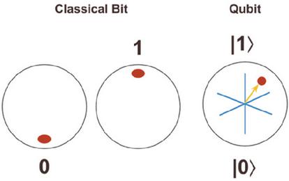
Figure 1 Classical bit and qubit.

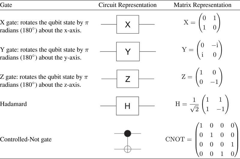
Quantum gates are analogous to processing instructions in quantum computers. They have mathematical properties as a unitary matrix, maintaining a total probability that is always equal to 1. This research divided gates into two main types based on their function. Non-Entanglement Gates (Single-Qubit Gates) act on a single qubit and are used for superposition, phase adjustment, or parameterized rotation without entanglement with other qubits, while Entanglement Gates (Multi-Qubit Gates) act on two or more qubits to create entanglement, establishing quantum relationships between them [31], as shown in Table 2.

Table 2 Standard quantum gates

3.2 Quantum Circuit and Unitary Operations

A quantum circuit is a model for quantum computing that uses a series of quantum gates connected together. Qubits are placed on wires, and these wires are acted upon by quantum gates. There are n qubits in total. Mathematically, the operation of a quantum circuit can be described by the unitary operation $\mathrm{U}$, which has the important property ${\mathrm{U}}^{†}\mathrm{U}=\mathrm{I}$, where ${\mathrm{U}}^{†}$ is the conjugate transpose of $\mathrm{U}$ and $\mathrm{I}$ is the identity matrix [32]. For the initial state $|{\psi }_{\mathrm{in}}⟩$, the resulting state after passing through the circuit $|{\psi }_{\mathrm{out}}⟩$ is calculated by:

$${\mathbf{|}\mathit{\psi }\mathbf{⟩}}_{\text{out}}=\text{U}(\mathit{\theta })|{\mathit{\psi }}_{\text{in}}⟩$$

(2)

This research focused on Variational Quantum Circuits (VQC) or PQCs, where $\mathrm{U}(\theta )$ is a function of the parameter $\theta$ that can be optimized by classical algorithms such as Gradient Descent to reduce the loss function of the system [33]. VQC or PQCs are fundamental components of modern QML algorithms, including QCNN. The structure of a VQC consists of a quantum circuit U($\theta$) that depends on a set of trainable parameters $\theta$. The operation of a VQC can be represented by:

$$\mathbf{|}\mathit{\psi }(\text{x},\mathit{\theta }\mathbf{)}\mathbf{⟩}=\text{U}\mathbf{(}\mathit{\theta }\mathbf{)}\mathbf{|}\mathit{\varphi }(\text{x})\mathbf{⟩}$$

(3)

where $|\varphi (\mathrm{x})⟩$ is the initial state obtained from classical data encoding and $\mathrm{U}(\theta )$ is a circuit consisting of rotation gates and entanglement gates. The goal is to find the best value of $\theta$ through classical optimization to reduce the loss function [33].

3.3 Expressibility

Expressibility is defined as the measure of a quantum circuit’s capability to generate quantum states that are uniformly distributed across the Hilbert space, relative to the distribution of Haar random states [18]. Mathematically, the expressibility of a PQC is quantified using the Kullback-Leibler (KL) divergence between the fidelity distribution of the circuit ${\mathrm{P}}_{\mathrm{PQC}}$ and the Haar random distribution (${\mathrm{P}}_{\mathrm{Haar}}$), as shown in Equation (4):

$$\text{Expr}={\text{D}}_{\text{KL}}({\text{P}}_{\text{PQC}}(\text{F})\mathbf{\parallel }{\text{P}}_{\text{Haar}}(\text{F}))$$

(4)

In this context, $\mathrm{F}={|⟨{\psi }_{\theta }|{\psi }_{\varphi }⟩|}^2$ represents the fidelity between two states generated by the circuit with randomly selected parameters $\theta$ and $\varphi$. A lower expressibility score signifies that the circuit distribution closely matches the Haar distribution, indicating high circuit expressibility, as shown in Figure 2.

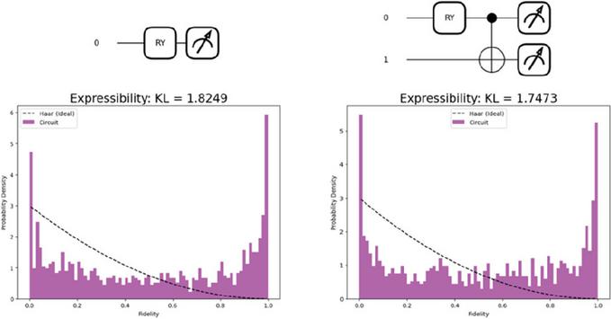
Figure 2 Expressibility analysis of different quantum circuit configurations using Kullback-Leibler (KL) divergence. The values shown are from the simulation.

3.4 Entanglement Capability

Entanglement capability (Ent) quantifies the ability of a quantum circuit to generate entanglement between qubits, which is a fundamental resource for capturing complex correlations within data. This property is typically assessed using the Meyer-Wallach measure ($\mathrm{Q}$), The average entanglement capability over the parameter space $\theta$ is defined as [18, 34]:

$$\text{Ent}=\frac{\mathbf{1}}{\mathbf{|}\text{S}\mathbf{|}}\sum _{\mathit{\theta }\in \text{S}}\text{Q}(\mathbf{|}{\mathit{\psi }}_{\mathit{\theta }}\mathbf{⟩})$$

(5)

The Meyer-Wallach measure $Q$ for a given quantum state $|\psi ⟩$ is derived from the purity of the reduced density matrix (${\rho }_k$) of each individual qubit, expressed as:

$$\text{Q}\mathbf{(}\mathbf{|}\mathit{\psi }\mathbf{⟩}\mathbf{)}=\mathbf{2}\left(\mathbf{1}-\frac{\mathbf{1}}{\text{n}}\sum _{\text{k}=\mathbf{0}}^{\text{n}-\text{1}}\mathrm{Tr}({\mathit{\rho }}_{\text{k}}^{\mathbf{2}})\right)$$

(6)

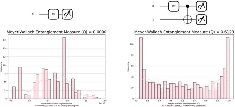
Figure 3 Evaluation of entangling capability for different quantum circuits using the Meyer-Wallach entanglement measure. The values shown are from the simulation.

Higher values of entanglement capability indicate a greater capacity of the circuit to entangle qubits, thereby enhancing the model’s ability to represent multi-variable relationships, as shown in Figure 3.

3.5 Classification Performance

Metrics that can reflect both the overall accuracy and address class asymmetry are used to evaluate a model’s ability to classify data. This study used accuracy and classification reports as the primary tools to measure model performance.

3.5.1 Accuracy

$$\mathrm{Accuracy}=\frac{\text{TP}+\text{TN}}{\text{TP}+\text{TN}+\text{FP}+\text{FN}}$$

(7)

3.5.2 Recall

$$\mathrm{Recall}=\frac{\text{TP}}{\text{TP}+\text{FN}}$$

(8)

3.5.3 Precision

$$\mathrm{Precision}=\frac{\text{TP}}{\text{TP}+\text{FP}}$$

(9)

3.5.4 F1-score

$$\text{F1-score}=\text{2}\times \frac{\mathrm{Precision}\times \mathrm{Recall}}{\mathrm{Precision}+\mathrm{Recall}}$$

(10)

4 Proposed Methodology

The research methodology used to develop and evaluate the performance of QNNs for chest radiographic image classification covered data preparation, model architecture, and the design of seven different quantum circuit types.

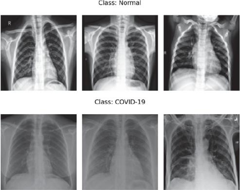
Figure 4 Examples of X-ray images from the dataset, including Normal and COVID-19.

4.1 Dataset Preparation

This study classified chest X-ray images to detect the presence of COVID-19. Lesions often appear as unique features on chest photographs, specifically as abnormalities in the lower lobes of the lungs, and as scatterings of frosted, mirror-like white patches near the edges of the lungs. This research used a dataset of chest X-ray images divided into two classes as patients with coronavirus disease and healthy people. Figure 4 shows 484 images, divided into 346 images for training, 88 images for validation, and 50 images for testing. After model training, the test was conducted using a new, never-before-seen dataset of 600 images.

4.2 Quantum Neural Network Model

The chest X-ray images were first resized to 64 $\times$ 64 pixels and 128 $\times$ 128 pixels, then converted to grayscale and adjusted to a 1D vector format suitable for model input. After resizing, the images were converted to a quantum state using amplitude encoding. This method replaced the classical data with qubits, enabling processing within quantum circuits. The 64 $\times$ 64 pixel images used 12 qubits, and the 128 $\times$ 128 pixel images used 14 qubits. The data were then passed through a variable quantum layer and analyzed, processed, and classified as normal or infected with COVID-19, as shown in Figure 5. The model parameters are shown in Table 3.

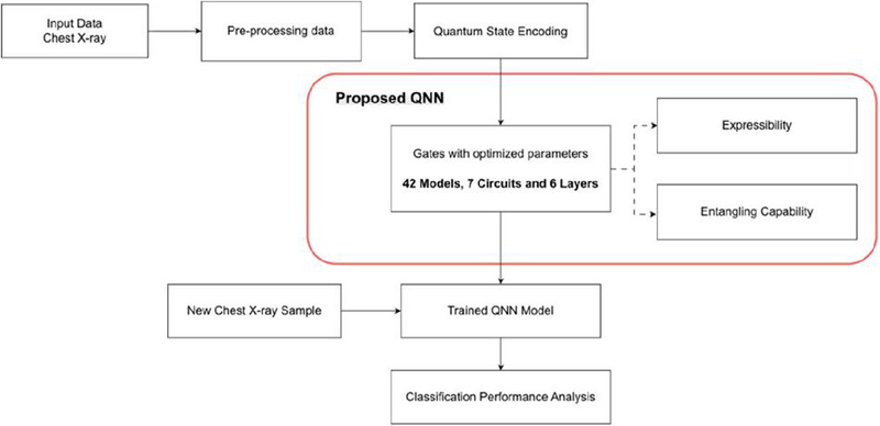
Figure 5 Proposed QNN model architecture for chest X-ray image classification.

Table 3 Parameters of the model

Parameter Name	Value
Learning rate	0.01
Batch size	4
Epochs	30
Optimizer	Adam
Loss Function	MSELoss
Quantum Library	PennyLane
QML Device	lightning.qubit
Framework	PyTorch
Programming Language	Python

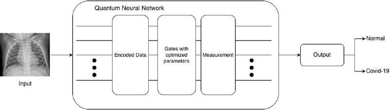
Figure 6 Proposed framework for chest X-ray classification using QNN.

Figure 6 shows the system workflow. The images were input and underwent initial processing. The data were then encoded into a quantum format. This experiment tested seven different QNN models, with each circuit tested across six layers to measure performance in three main areas as expressibility, entangling capability, and accuracy. After training, the models were tested against previously unseen data. Finally, the image classification results were summarized, and the accuracy was evaluated using various metrics.

The seven circuit models were designed from a basic circuit with only a single-qubit gate using the Rotation Y gate. This gate could accept parameters for adjustment during the learning process. The complexity was then increased by applying CNOT gates to create entanglement, and analyze how the creation of quantum relationships between qubits increased the accuracy of complex data classification compared to the basic circuit model, as shown in Figure 7.

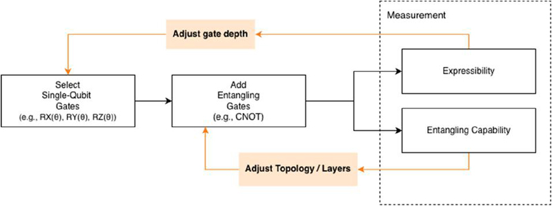
Figure 7 Iterative framework for quantum circuit optimization based on expressibility and entangling capability.

Table 4 Variable quantum circuits used in QNN models

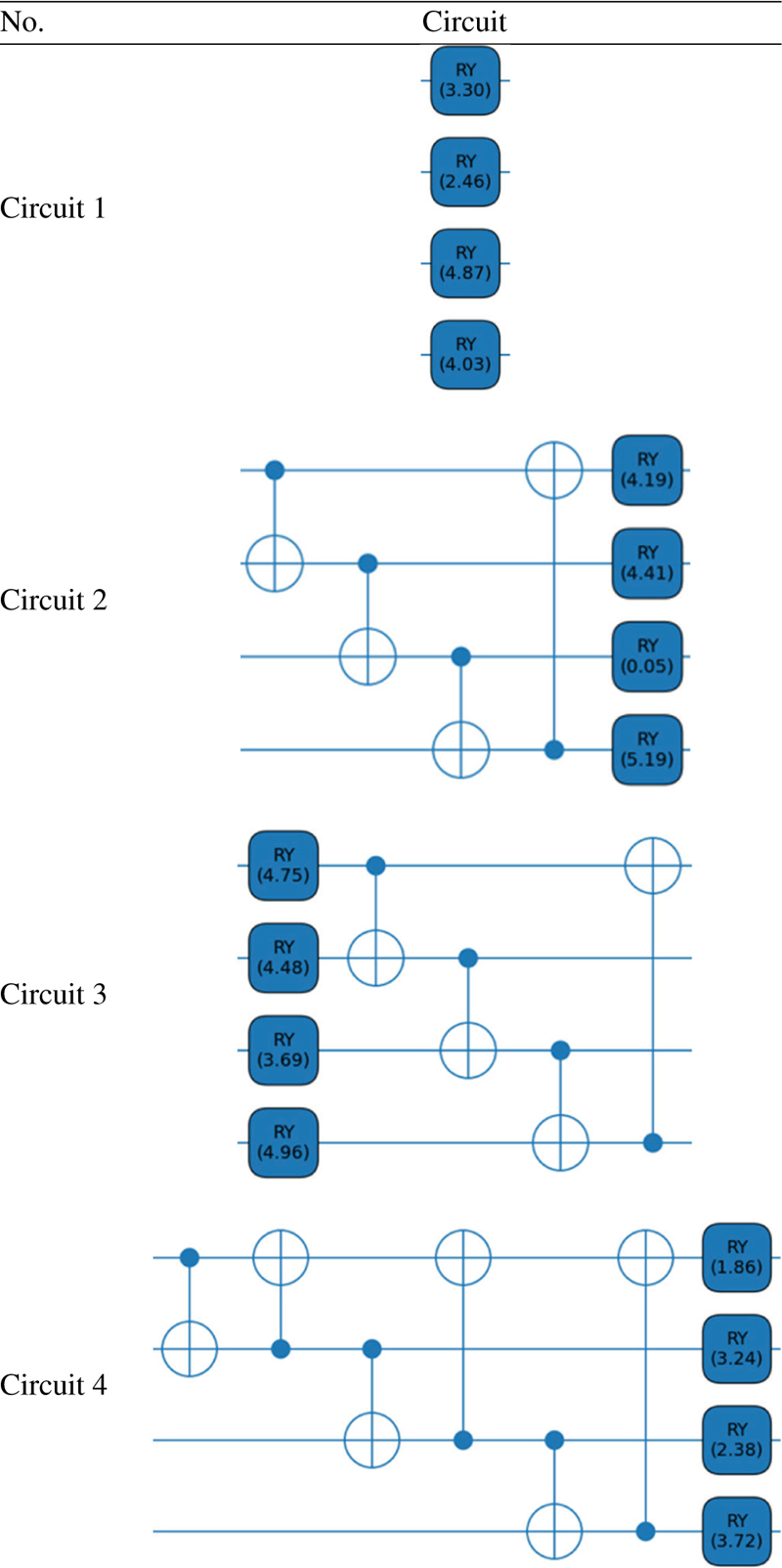
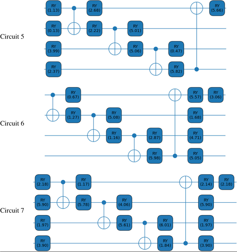
Table 4 shows the different layouts as follows:

• Circuit 1: This circuit placed only Rotation Gate Y (RY) in parallel on all qubits, without using CNOT Gates to create entanglement.

• Circuit 2: This circuit placed CNOT Gates in a chain, connecting backward from the last to the first to create entanglement. Thereafter, Rotation Gate Y (RY) was placed on all qubits.

• Circuit 3: This circuit reversed the order of placement from circuit 2, placing Rotation Gate Y (RY) at the very front to adjust the qubit state first, followed by placing CNOT Gates in a chain, connecting backward from the last to the first.

• Circuit 4: This circuit increased the complexity of entanglement by placing two layers of CNOT Gates (e.g., 1–2 with 3–4 and backward) to allow for more intensive data exchange first. Thereafter, Rotation Gate Y (RY) was placed on all qubits.

• Circuit 5: This circuit was similar to circuit 3, but for each pair of CNOT Gates, a Rotation Gate Y (RY) was added at each level of the qubit. A Rotation Gate Y (RY) was then placed on the first qubit of each qubit.

• Circuit 6: Similar to the layout in method 2, each pair of CNOT Gates had a Rotation Gate Y (RY) added at each level of the qubit. Then, a Rotation Gate Y (RY) was placed on the first qubit of each qubit.

• Circuit 7: This layout was the most complex and used the most gates, with Rotation Gate Y (RY) placed both before and after the CNOT Gate at every connection point.

Table 5 shows the workflow of the algorithm for classifying X-ray images, beginning with image preprocessing, followed by feature mapping into a quantum state using amplitude encoding. Processing then proceeded through the seven defined VQCs, with a circuit depth of six layers. Finally, the image was classified as either COVID-19 or normal.

Table 5 Algorithm QNN for X-ray image classification

Input: Chest X-Ray Image Dataset

Procedure

1. Preprocessing: Resize image, convert to Grayscale, and Normalize.

2. For each epoch $\mathrm{e}\in \{1,\mathrm{\dots },E=30\}$ do: • Data are encoded into the amplitudes of a quantum state. • Variational Quantum Circuit Layer Configuration: l $=$ {1, 2, 3, 4, 5, 6} VQC: shown in Table 4 • Measurement: Measure the expectation value Z of the first qubit to obtain a scalar output between [$-$1, 1]. • Classification: Map the output to class labels where $-$1 $=$ COVID-19, 1 $=$ Normal. • Optimization: Calculate Mean Squared Error (MSE) Loss. Compute gradients using the parameter-shift rule. Update quantum weights $\theta$ using the Adam Optimizer.

3. Output: Trained Model and Classification Labels.

4.3 Quantum Convolutional Neural Network Model

The QCNN process began with data preparation for model input. The images were resized to 64 $\times$ 64 pixels and 128 $\times$ 128 pixels, converted to grayscale, and then encoded to a quantum state using amplitude encoding. Next, the convolution and pooling circuits were defined as shown in Figure 9, with 2 qubits used for both the convolution and pooling circuits. Finally, the data were sent to the Fully Connected (FC) layer for analysis, processing, and classification as normal or infected with COVID-19, as shown in Figure 8. The model parameters are shown in Table 3.

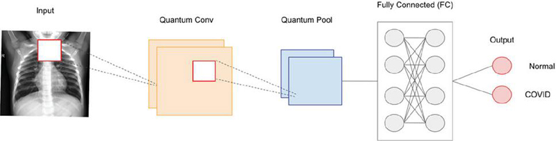
Figure 8 Proposed QCNN model architecture for chest X-ray image classification.

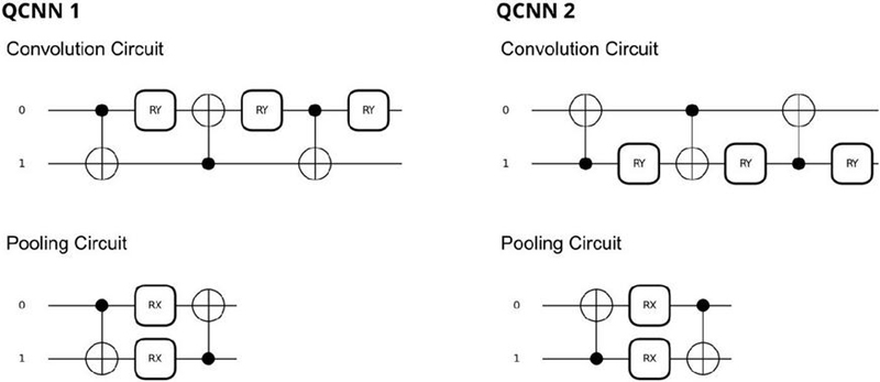
Figure 9 Gate configurations for quantum convolutional and pooling layers of QCNN.

5 Results and Discussion

The model performance tests covered two image sizes as 64 $\times$ 64 pixels and 128 $\times$ 128 pixels. The accuracy, precision, recall, and F1-score comparisons for each image size are detailed in Tables 6–10 and 11–15. Tests were also conducted in QCNN using 64 $\times$ 64 and 128 $\times$ 128 pixel image sizes, as shown in Table 16.

Table 6 Performance evaluation for a 64 $\times$ 64 pixel image dataset

	Accuracy
Model	1 Layer	2 Layer	3 Layer	4 Layer	5 Layer	6 Layer
QNN 1	32.00%	68.00%	68.00%	68.00%	36.00%	60.00%
QNN 2	56.00%	80.00%	96.00%	92.00%	92.00%	96.00%
QNN 3	80.00%	96.00%	100.00%	96.00%	96.00%	96.00%
QNN 4	32.00%	88.00%	84.00%	92.00%	96.00%	88.00%
QNN 5	92.00%	84.00%	92.00%	100.00%	100.00%	96.00%
QNN 6	72.00%	84.00%	100.00%	96.00%	100.00%	100.00%
QNN 7	96.00%	96.00%	88.00%	100.00%	100.00%	100.00%

Table 7 Precision evaluation for a 64 $\times$ 64 pixel image dataset

	Precision
Model	1 Layer	2 Layer	3 Layer	4 Layer	5 Layer	6 Layer
QNN 1	0.21	0.73	0.73	0.73	0.23	0.76
QNN 2	0.28	0.84	0.97	0.94	0.94	0.97
QNN 3	0.84	0.97	1.00	0.97	0.97	0.97
QNN 4	0.18	0.89	0.84	0.94	0.97	0.91
QNN 5	0.94	0.89	0.94	1.00	1.00	0.97
QNN 6	0.76	0.84	1.00	0.97	1.00	1.00
QNN 7	0.97	0.97	0.89	1.00	1.00	1.00

Table 8 Recall evaluation for a 64 $\times$ 64 pixel image dataset

	Recall
Model	1 Layer	2 Layer	3 Layer	4 Layer	5 Layer	6 Layer
QNN 1	0.29	0.70	0.70	0.70	0.32	0.64
QNN 2	0.50	0.82	0.95	0.91	0.91	0.95
QNN 3	0.82	0.95	1.00	0.95	0.95	0.95
QNN 4	0.36	0.89	0.85	0.91	0.95	0.86
QNN 5	0.91	0.82	0.91	1.00	1.00	0.95
QNN 6	0.74	0.85	1.00	0.95	1.00	1.00
QNN 7	0.95	0.95	0.89	1.00	1.00	1.00

Table 9 F1-score evaluation for a 64 $\times$ 64 pixel image dataset

	F1-score
Model	1 Layer	2 Layer	3 Layer	4 Layer	5 Layer	6 Layer
QNN 1	0.32	0.68	0.68	0.68	0.36	0.60
QNN 2	0.56	0.80	0.96	0.92	0.92	0.96
QNN 3	0.80	0.96	1.00	0.96	0.96	0.96
QNN 4	0.32	0.88	0.84	0.92	0.96	0.88
QNN 5	0.92	0.84	0.92	1.00	1.00	0.96
QNN 6	0.72	0.84	1.00	0.96	1.00	1.00
QNN 7	0.96	0.96	0.88	1.00	1.00	1.00

Table 10 Performance evaluation for a 64 $\times$ 64 pixel image dataset tested with 600 images

	Accuracy
Model	1 Layer	2 Layer	3 Layer	4 Layer	5 Layer	6 Layer
QNN 1	25.17%	75.17%	75.50%	67.50%	27.83%	71.00%
QNN 2	50.00%	81.00%	91.33%	91.00%	93.83%	91.83%
QNN 3	91.00%	89.83%	94.50%	93.83%	91.33%	94.67%
QNN 4	42.17%	83.00%	89.50%	89.00%	91.17%	93.83%
QNN 5	94.67%	91.50%	93.50%	94.17%	93.50%	94.50%
QNN 6	76.83%	93.83%	94.33%	94.67%	91.83%	91.67%
QNN 7	95.00%	94.00%	94.83%	88.33%	92.33%	94.50%

Table 11 Performance evaluation for a 128 $\times$ 128 pixel image dataset

	Accuracy
Model	1 Layer	2 Layer	3 Layer	4 Layer	5 Layer	6 Layer
QNN 1	32.00%	72.00%	68.00%	32.00%	52.00%	68.00%
QNN 2	56.00%	80.00%	92.00%	100.00%	92.00%	96.00%
QNN 3	80.00%	80.00%	80.00%	80.00%	92.00%	92.00%
QNN 4	40.00%	72.00%	84.00%	80.00%	88.00%	80.00%
QNN 5	92.00%	96.00%	100.00%	100.00%	92.00%	100.00%
QNN 6	72.00%	92.00%	96.00%	88.00%	92.00%	100.00%
QNN 7	88.00%	96.00%	100.00%	96.00%	100.00%	100.00%

Table 12 Precision evaluation for a 128 $\times$ 128 pixel image dataset

	Precision
Model	1 Layer	2 Layer	3 Layer	4 Layer	5 Layer	6 Layer
QNN 1	0.21	0.76	0.73	0.21	0.27	0.73
QNN 2	0.28	0.84	0.94	1.00	0.94	0.97
QNN 3	0.80	0.80	0.80	0.80	0.94	0.94
QNN 4	0.41	0.76	0.87	0.80	0.91	0.80
QNN 5	0.94	0.97	1.00	1.00	0.94	1.00
QNN 6	0.76	0.94	0.97	0.91	0.94	1.00
QNN 7	0.91	0.97	1.00	0.97	1.00	1.00

Table 13 Recall evaluation for a 128 $\times$ 128 pixel image dataset

	Recall
Model	1 Layer	2 Layer	3 Layer	4 Layer	5 Layer	6 Layer
QNN 1	0.29	0.74	0.70	0.29	0.46	0.70
QNN 2	0.50	0.82	0.91	1.00	0.91	0.95
QNN 3	0.79	0.79	0.79	0.79	0.91	0.91
QNN 4	0.43	0.74	0.86	0.79	0.86	0.79
QNN 5	0.91	0.95	1.00	1.00	0.91	1.00
QNN 6	0.74	0.91	0.95	0.86	0.91	1.00
QNN 7	0.86	0.95	1.00	0.95	1.00	1.00

Table 14 F1-score evaluation for a 128 $\times$ 128 pixel image dataset

	F1-score
Model	1 Layer	2 Layer	3 Layer	4 Layer	5 Layer	6 Layer
QNN 1	0.32	0.72	0.68	0.32	0.52	0.68
QNN 2	0.56	0.80	0.92	1.00	0.92	0.96
QNN 3	0.80	0.80	0.80	0.80	0.92	0.92
QNN 4	0.40	0.72	0.84	0.80	0.88	0.80
QNN 5	0.92	0.96	1.00	1.00	0.92	1.00
QNN 6	0.72	0.92	0.96	0.88	0.92	1.00
QNN 7	0.88	0.96	1.00	0.96	1.00	1.00

Table 15 Performance evaluation for a 128 $\times$ 128 pixel image dataset tested with 600 images

	Accuracy
Model	1 Layer	2 Layer	3 Layer	4 Layer	5 Layer	6 Layer
QNN 1	26.33%	76.67%	74.33%	26.50%	30.17%	69.83%
QNN 2	50.00%	84.33%	88.17%	91.33%	90.83%	90.50%
QNN 3	91.00%	91.50%	92.83%	91.50%	92.00%	92.17%
QNN 4	42.67%	86.50%	87.33%	83.17%	87.50%	88.33%
QNN 5	93.17%	93.00%	93.00%	92.67%	93.50%	94.17%
QNN 6	77.33%	88.83%	93.83%	92.50%	93.83%	94.00%
QNN 7	94.00%	92.83%	94.17%	94.33%	92.83%	95.00%

Table 16 Performance evaluation for QCNN

		Accuracy		Expressibility		Entangling Capability
No.	Image Size	50	600	Conv	Pooling	Conv	Pooling
QCNN 1	64 $\times$ 64	96.00%	94.00%	0.1868	12.0237	0.1490	0.2358
	128 $\times$ 128	96.00%	93.17%
QCNN 2	64 $\times$ 64	98.00%	94.33%	0.1867	12.0237	0.1514	0.2413
	128 $\times$ 128	94.00%	93.67%

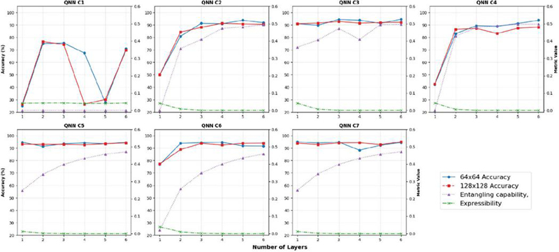
Figure 10 Expressibility, entangling capability, and performance analysis of seven 7-circuit architectures at 6-layer depth.

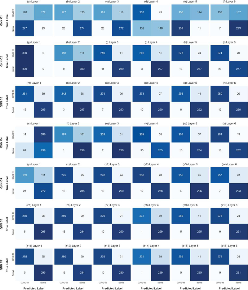
Figure 11 Confusion matrix for 64 $\times$ 64 pixel input images.

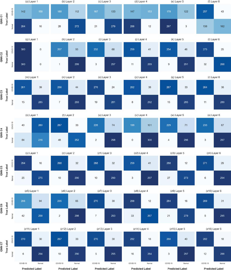
Figure 12 Confusion matrix for 128 $\times$ 128 pixel input images.

Figure 10 compares the accuracy of different models using different circuits. In QNNs, the number of layers or circuit complexity significantly affects model accuracy, as shown by the confusion matrices in Figures 11 and 12, with lower circuit complexity resulting in lower accuracy. However, the gate arrangement also impacts accuracy. Circuits 2, 4, and 6, all with a single-layer arrangement, exhibited low accuracy. These circuits shared the common characteristic of starting with the CNOT gate before Ry, a parameter-accepting gate. Conversely, circuits 3, 5, and 7 placed Ry before the CNOT gate. Learning began in layer 1, and increasing the number of layers improved learning and accuracy, highlighting the importance of preparing the circuit state before entanglement for optimal model learning.

Table 17 Training time for 64 $\times$ 64 pixels

	Training Time (minutes)
Model	1 Layer	2 Layer	3 Layer	4 Layer	5 Layer	6 Layer
QNN 1	3.64	5.52	7.77	11.95	15.92	22.22
QNN 2	4.24	24.44	62.65	114.78	187.79	282.49
QNN 3	13.61	42.84	90.21	147.16	239.06	348.91
QNN 4	4.90	32.07	81.48	155.21	256.64	391.97
QNN 5	40.45	160.45	370.37	660.22	1627.02	2140.01
QNN 6	28.89	137.11	413.44	740.62	1441.03	2017.91
QNN 7	56.32	375.89	661.56	1,182.86	2223.23	3158.77

Table 18 Training time for 128 $\times$ 128 pixels

	Training Time (minutes)
Model	1 Layer	2 Layer	3 Layer	4 Layer	5 Layer	6 Layer
QNN 1	4.4	6.2	9.09	12.56	18.78	26.40
QNN 2	4.97	30.68	76.44	139.87	285.43	424.53
QNN 3	16.317	51.97	105.9	191.04	364.54	604.32
QNN 4	5.48	37.44	98.25	178.77	457.15	618.37
QNN 5	57.35	246.32	587.22	1270.32	2435.79	3285.07
QNN 6	33.41	200.05	515.9	1163.76	2085.70	2976.93
QNN 7	73.31	375.88	904.44	1630.89	2622.25	3809.03

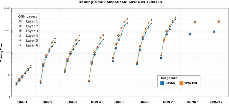
Figure 13 Comparison of training time between the proposed QNNs.

Tables 17–18 and Figure 13 compare the learning times of the models. QCNN took longer to learn than QNN due to the different architectural structures or operating principles. Factors such as image size, the number of gates, and the number of layers all affected the learning time. Increasing the image size and the number of qubits to match the image size resulted in similar learning times, because the quantum superposition property allows QCNN to handle higher-dimensional data by increasing the number of qubits to match the image size.

Table 19 Comparison of expressibility for QNNs

Model	Expressibility
	1 Layer	2 Layer	3 Layer	4 Layer	5 Layer	6 Layer
QNN 1	0.0414	0.0426	0.0432	0.0395	0.0398	0.0426
QNN 2	0.0408	0.0081	0.0002	0	0	0
QNN 3	0.0416	0.0065	0.0002	0	0	0
QNN 4	0.0428	0.0058	0.0001	0	0	0
QNN 5	0.0119	0.0022	0.0004	0	0	0
QNN 6	0.0387	0.0093	0.0017	0.0004	0	0
QNN 7	0.0115	0.0019	0.0001	0.0001	0	0

Table 20 Comparison of entangling capability for QNNs

Model	Entangling Capability
	1 Layer	2 Layer	3 Layer	4 Layer	5 Layer	6 Layer
QNN 1	0	0	0	0	0	0
QNN 2	0	0.357	0.4089	0.4727	0.4817	0.4942
QNN 3	0.3639	0.4065	0.4723	0.4096	0.4943	0.4963
QNN 4	0	0.4285	0.4779	0.4884	0.4964	0.4980
QNN 5	0.2487	0.3416	0.3989	0.4334	0.4572	0.4711
QNN 6	0.0206	0.2572	0.3488	0.4006	0.4358	0.4585
QNN 7	0.2494	0.3446	0.399	0.4344	0.4567	0.4720

In terms of expressibility, a value approaching 0 indicated good coverage of the Hilbert space, and an entangling capability approaching 1 indicated high entanglement or interconnectedness between qubits, as shown in Tables 19 and 20. Most models (QNN 2–7) showed a rapid decrease in expressibility as the number of layers increased, especially at 4–6 layers, where the value approached 0. This demonstrated that increasing depth allowed the circuit to reach the widest range of states. Regarding entangling capability, all the models except QNN 1 showed a significant increase in entanglement with increasing layer numbers, consistent with the theory that depth increased qubit interactions. QNN 1’s entangling capability remained 0 across all layers because its gate configuration lacked entanglement, thus preventing qubit interconnectedness. Circuits 2 and 4 are interesting because they both started at 0 in layer 1 due to the circuit’s non-entangled state caused by placing the CNOT gate before Ry, and highlighting the importance of gate placement order.

Experimental results confirmed the importance of designing circuits with high entanglement capability and expressibility to optimize the QNN model. A highly efficient circuit should have a low expressibility value (close to 0), meaning that the circuit can randomize states in a more comprehensive Hilbert space. As the number of layers increased, expressibility values decreased and remained at very low levels, reflecting how circuit depth improved the model’s ability to accurately represent data, as shown in Figures 14 and 15. The circuit also had a high entanglement capability, with C2, C3, C4, and C7 demonstrating higher classification efficiency when the entanglement factor increased with the number of layers, resulting in higher accuracy for both the 64 $\times$ 64 and 128 $\times$ 128 resolutions. In the C5, C6, and C7 circuits, the entanglement values did not reach their maximum in the early layers. However, the model had high values from the first 1–2 layers, showing that, for the gate arrangement structure, these circuits were more efficient for feature extraction.

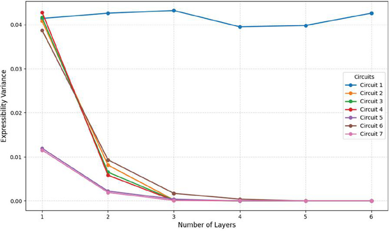
Figure 14 Comparison of expressibility for QNNs.

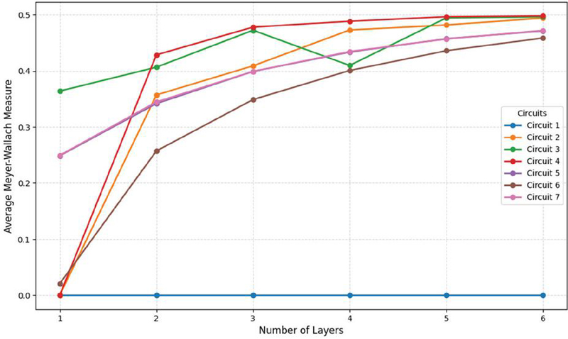
Figure 15 Comparison of entangling capability for QNNs.

Table 21 Comparison with other related research

			Datasets						Circuit Analysis
						Image			Trainable	Time for		Entanglement
Name	Models	Classification	Training	Validation	Test	Size (Pixel)	Qubit	Accuracy	Parameters	Training	Exprssibility	Capability
	NN	COVID-19	346	88	50	128 $\times$ 128	–	100.00%	25,298,178	1m 52s
					600			95.00%
	VGG16	COVID-19	346	88	50	128 $\times$ 128	–	96.00%	119,554,050	6m 42s
					600			92.00%
[21]	Pre-trained models (ResNet50 and VGG16)	CT Scan	9,500	1,500	224 $\times$ 224	16	96.92%	32	52m
[26]	HQ-CNN	Chest X-ray	180	120	256 $\times$ 256	4	94.20%	6	N/A
[28]	QML	Chest X-ray	70%	15%	15%	224 $\times$ 224	8	88.40%	8	N/A
This study	QCNN	COVID-19	346	88	50	64 $\times$ 64	4 (2-qubit	96.00%	10	118 m	$\surd$	$\surd$
	(Balancing					128 $\times$ 128	conv and	96.00%
	Quantum				600	64 $\times$ 64	2-qubit pooling)	96.00%
	Circuit: 2 Models, 4 Circuits)					128 $\times$ 128		94.33%
	QNN				50	64 $\times$ 64	12	100.00%	14–246	3 m–3,809 m
	(Balancing					128 $\times$ 128	16	100.00%
	Quantum				600	64 $\times$ 64	12	96.00%
	Circuit: 42 Models, 7 Circuits)					128 $\times$ 128	16	94.33%

Table 21 compares this research with previous research using similar datasets. Analysis revealed that even though this experiment used higher resolution or sized images, resulting in a corresponding increase in the number of gates in the circuit, the accuracy results remained satisfactory.

Most previous research focused solely on measuring accuracy performance. However, this research studied additional circuit capability indicators by using expressibility and entanglement capability to enable an in-depth relationship analysis and select the most suitable circuit design for the studied model. Experiments were conducted with various image sizes to study the impact of the number of gates on processing performance. The number of gates depended on the image size, and the dataset used was a crucial factor affecting the learning performance and future scalability of the model.

6 Conclusions, Limitations, and Future Work

6.1 Conclusions

This research presented a QNN for classifying COVID-19 X-ray images. The investigation encompassed seven distinct circuits, with both entangled and non-entangled configurations, each subjected to evaluation across six supplementary layers. The results indicated that augmenting the layer count within a QNN model correlated with enhanced accuracy. The introduction of an excessive number of layers precipitated overfitting, demonstrating that each circuit had an optimal number of layers for its model, and the number of layers to add depended on the circuit and the desired objective for improving model performance. In quantum circuit analysis, expressibility is a key factor for entanglement. High expressibility but low entanglement may affect model learning, while high expressibility but low or no entanglement may result in inefficient model learning compared to circuits with balanced expressibility and entanglement. Therefore, a good or efficient circuit should have a balanced relationship between expressibility and entanglement. The experimental results showed that QNNs learn faster than QCNNs because QNNs have a more flexible and less complex structure. Therefore, QNNs serve as a favorable entry point for initial studies, enabling rapid experimentation and parameter tuning to better understand quantum behaviors and model dynamics under current resource constraints.

6.2 Limitations

This research was developed using simulations on PennyLane however, a physical hardware system will have the potential to encounter noise and quantum decoherence resulting from environmental interactions and imperfect controls. If the circuit depth becomes excessive or qubits remain in an idle state for too long, the data will be interfered with, which will lead to a reduction in efficiency. Currently, Quantum Error Correction (QEC) is being developed to address these issues by distributing information across multiple qubits to create entanglement for data protection [35, 36].

6.3 Future Work

Future research should apply circuit design principles to develop new models that are flexible and aligned with future advancements. Since this study relies on ideal simulations, future work must account for hardware noise and decoherence. Additionally, expanding dataset volume and diversity is essential to enhance generalization and mitigate overfitting risks [35, 36]. In addition, the analytical challenges of quantum computing using QML in Thailand are being driven across many applications in healthcare, materials science, logistics, and financial modeling [37].

References

[1] Sameer I. Ali Al-Janabi et al., “An Enhanced Convolutional Neural Network for COVID-19 Detection,” Intelligent Automation & Soft Computing, vol. 28, no. 2, pp. 293–303, 2021, doi:10.32604/iasc.2021.014419.

[2] E. H. Houssein, Z. Abohashima, M. Elhoseny, and W. M. Mohamed, “Hybrid Quantum-Classical Convolutional Neural Network Model for COVID-19 Prediction using Chest X-Ray Images,” J Comput Des Eng, vol. 9, no. 2, pp. 343–363, Apr. 2022, doi:10.1093/jcde/qwac003.

[3] H. Allioui et al., “A Multi-Agent Deep Reinforcement Learning Approach for Enhancement of COVID-19 CT Image Segmentation,” J Pers Med, vol. 12, no. 2, 2022, doi:10.3390/jpm12020309.

[4] M. Mahmood, W. J. Al-Kubaisy, and B. Al-Khateeb, “Review of IoT for COVID-19 Detection and Classification,” in International Conference on Innovative Computing and Communications, A. Khanna, D. Gupta, S. Bhattacharyya, A. E. Hassanien, S. Anand, and A. Jaiswal, Eds., Singapore: Springer Singapore, pp. 859–872, 2022.

[5] I. F. Jassam, S. M. Elkaffas, and A. A. El-Zoghabi, “Chest X-Ray Pneumonia Detection by Dense-Net,” in 2021 31st International Conference on Computer Theory and Applications (ICCTA), Alexandria, Egypt, pp. 176–179, 2021, doi:10.1109/ICCTA54562.2021.9916637.

[6] E. Çallı, E. Sogancioglu, B. van Ginneken, K. G. van Leeuwen, and K. Murphy, “Deep Learning for Chest X-Ray Analysis: A Survey,” Med Image Anal, vol. 72, p. 102125, 2021, doi: https://doi.org/10.1016/j.media.2021.102125.

[7] S. Anand, R. K. Roshan, and D. Sundaram, “Chest X-Ray Image Enhancement using Deep Contrast Diffusion Learning,” Optik (Stuttg), vol. 279, p. 170751, 2023, doi: https://doi.org/10.1016/j.ijleo.2023.170751.

[8] A. Leelasantitham, “A Novel Guideline Framework for Research and Development in the Field of Management of Technology and Innovation,” in 2024 5th Technology Innovation Management and Engineering Science International Conference (TIMES-iCON), pp. 1–5, 2024, doi:10.1109/TIMES-iCON61890.2024.10630775.

[9] M. A. Yenikaya, G. Kerse, and O. Oktaysoy, “Artificial Intelligence in the Healthcare Sector: Comparison of Deep Learning Networks using Chest X-Ray Images,” Front Public Health, vol. 12, 2024, doi:10.3389/fpubh.2024.1386110.

[10] Y. H. Bhosale and K. S. Patnaik, “Bio-Medical Imaging (X-ray, CT, ultrasound, ECG), Genome Sequences Applications of Deep Neural Network and Machine Learning in Diagnosis, Detection, Classification, and Segmentation of COVID-19: A Meta-analysis & Systematic Review,” Multimed Tools Appl, vol. 82, no. 25, pp. 39157–39210, 2023, doi:10.1007/s11042-023-15029-1.

[11] P.K. Illa, T. Senthil Kumar, and F. Syed Anwar Hussainy, “Deep Learning Methods for Lung Cancer Nodule Classification: A Survey,” Journal of Mobile Multimedia vol. 18, pp. 421–450, 2022, https://doi.org/10.13052/jmm1550-4646.18213.

[12] R. Idzikowski, M. A. Kucharski, K. Pempera, and M. Jaroszczuk, “A Survey on Quantum Machine Learning Applications in Medicine and Healthcare,” Multidisciplinary Digital Publishing Institute (MDPI), 1 Feb. 2026, doi:10.3390/app16031630.

[13] D. Jain, S. Hundekari, K. Upreti, N. Jain, M. Rose, N. Singh, R. Singhai, and M. Kumar, “RCBAM-CNN: Rebuild Convolution Block Attention Module-based Convolutional Neural Network for Lung Nodule Classification,” Journal of Mobile Multimedia, vol. 20, pp. 1039–1066, 2024, https://doi.org/10.13052/jmm1550-4646.2053.

[14] A. I. Khan, J. L. Shah, and M. M. Bhat, “CoroNet: A Deep Neural Network for Detection and Diagnosis of COVID-19 from Chest X-Ray Images,” Comput Methods Programs Biomed, vol. 196, Nov. 2020, doi:10.1016/j.cmpb.2020.105581.

[15] R. K. Gupta et al., “Novel Deep Neural Network Technique for Detecting Environmental Effect of COVID-19,” Energy Sources, Part A: Recovery, Utilization and Environmental Effects, vol. 47, no. 1, pp. 8997–9015, 2025, doi:10.1080/15567036.2021.1941435.

[16] S. Shomir Dutta, S. Sandeep, S. Sridevi, R. Mistry, J. Ortega, and G. Kar, “Novel Quanvolutional Neural Network-Based COVID-19 Diagnosis From Raman Spectroscopic Signals of Human Serum,” IEEE Access, vol. 13, pp. 104382–104405, 2025, doi:10.1109/ACCESS.2025.3580316.

[17] W. El Maouaki, A. Marchisio, T. Said, M. Shafique, and M. Bennai, “Designing Robust Quantum Neural Networks via Optimized Circuit Metrics,” Advanced Quantum Technologies, 2025, https://doi.org/10.1002/qute.202400601.

[18] S. Sim, P. D. Johnson, and A. Aspuru-Guzik, “Expressibility and Entangling Capability of Parameterized Quantum Circuits for Hybrid Quantum-Classical Algorithms,” May 2019, doi:10.1002/qute.201900070.

[19] T. Hubregtsen, J. Pichlmeier, P. Stecher, and K. Bertels, “Evaluation of Parameterized Quantum Circuits: On the Relation between Classification Accuracy, Expressibility, and Entangling Capability,” Quantum Mach Intell, vol. 3, no. 1, p. 9, 2021, doi:10.1007/s42484-021-00038-w.

[20] M. M. Hossain, M. A. Rahim, A. N. Bahar, and M. M. Rahman, “Automatic Malaria Disease Detection from Blood Cell Images using the Variational Quantum Circuit,” Inform Med Unlocked, vol. 26, Jan. 2021, doi:10.1016/j.imu.2021.100743.

[21] K. Sengupta and P. R. Srivastava, “Quantum Algorithm for Quicker Clinical Prognostic Analysis: An Application and Experimental Study using CT Scan Images of COVID-19 Patients,” BMC Med Inform Decis Mak, vol. 21, no. 1, Dec. 2021, doi:10.1186/s12911-021-01588-6.

[22] Y. Zeng, H. Wang, J. He, Q. Huang, and S. Chang, “A Multi-Classification Hybrid Quantum Neural Network Using an All-Qubit Multi-Observable Measurement Strategy,” Entropy, vol. 24, no. 3, 2022, doi:10.3390/e24030394.

[23] H. Th. S. Alrikabi, I. A. Aljazaery, J. S. Qateef, A. H. M. Alaidi, and R. M. Al_airaji, “Face Patterns Analysis and Recognition System Based on Quantum Neural Network QNN,” International Journal of Interactive Mobile Technologies, vol. 16, no. 8, pp. 34-48, 2022, doi:10.3991/ijim.v16i08.30107.

[24] T. Nguyen, I. Paik, Y. Watanobe, and T. C. Thang, “An Evaluation of Hardware-Efficient Quantum Neural Networks for Image Data Classification,” Electronics (Basel), vol. 11, no. 3, 2022, doi: 10.3390/electronics11030437.

[25] Y. Li, R. Liu, X. Hao, R. Shang, P. Zhao, and L. Jiao, “EQNAS: Evolutionary Quantum Neural Architecture Search for Image Classification,” Neural Networks, vol. 168, pp. 471–483, 2023, doi: https://doi.org/10.1016/j.neunet.2023.09.040.

[26] A. Rana, D. K. Bhaglani, P. Vaidya, and Y. C. Hu, “Meta-Analysis of Quantum Convolutional Neural Networks for Automated Tuberculosis Screening on Chest X-Rays,” Multimed Tools Appl, vol. 84, pp. 40781–40807, 2025, https://doi.org/10.1007/s11042-025-20614-7.

[27] A. Dubey, T. Gantala, A. Ray, A. Prabhakar, and P. Rajagopal, “Quantum Machine Learning for Recognition of Defects in Ultrasonic Imaging,” NDT & E International, vol. 150, p. 103262, 2025, doi: https://doi.org/10.1016/j.ndteint.2024.103262.

[28] S. Rawas and D. AlSaeed, “Quantum Enhanced Machine Learning for Medical Image Analysis: A Hybrid Approach,” Applied Computing and Informatics, pp. 1–16, Jan. 2026, doi:10.1108/ACI-10-2025-0448.

[29] S. C. Kak, “Quantum Neural Computing,” in Advances in Imaging and Electron Physics, vol. 94, pp. 259–313, 1995, doi: https://doi.org/10.1016/S1076-5670(08)70147-2.

[30] R. Chrisley, “Quantum Learning,” in New Directions in Cognitive Science: Proceedings of the International Symposium, Saariselkä, Lapland, Finland, pp. 77–89, 1995.

[31] M. Möttönen and J. Vartiainen, “Decompositions of General Quantum Gates,” Frontiers in Artificial Intelligence and Applications, May 2005.

[32] J. Biamonte, P. Wittek, N. Pancotti, P. Rebentrost, N. Wiebe, and S. Lloyd, “Quantum Machine Learning,” Nature, vol. 549, Nov. 2016, doi:10.1038/nature23474.

[33] M. Schuld and F. Petruccione, Machine Learning with Quantum Computers, 2021, doi:10.1007/978-3-030-83098-4.

[34] D. A. Meyer and N. R. Wallach, Global Entanglement in Multiparticle Systems, 2001.

[35] R. Matsumoto and M. Hagiwara, “A Survey of Quantum Error Correction,” IEICE Transactions on Fundamentals of Electronics, Communications and Computer Sciences, vol. E104A, no. 12, pp. 1654–1664, 2021, doi:10.1587/transfun.2021EAI0001.

[36] A. Chatterjee, K. Phalak, and S. Ghosh, “Quantum Error Correction For Dummies,” Quantum Physics, Apr. 2023, doi:10.1109/QCE57702.2023.00162.

[37] N. Chaipunha, V. Panya, and A. Leelasantitham, “Analytical Challenges of Quantum and Classical Computing in Thailand: A Comparative Exploration of Machine Learning Through Classification,” in 2024 5th Technology Innovation Management and Engineering Science International Conference (TIMES-iCON), pp. 1–5, 2024, doi:10.1109/TIMES-iCON61890.2024.10630768.

Biographies

Amy Sungsiri received the B.Eng. degree in Computer Engineering and Artificial Intelligence and the M.Sc. degree in Information Technology from the Thai-Nichi Institute of Technology, Bangkok, Thailand, in 2020 and 2023, respectively. She is currently pursuing the Ph.D. degree in Information Technology Management with the Faculty of Engineering, Mahidol University. Her research interests primarily focus on the advancement of deep learning and quantum computing, specifically in the development of Convolutional Neural Networks (CNN), Quantum Neural Networks (QNN), and Quantum Convolutional Neural Networks (QCNN).

Adisorn Leelasantitham received the B.Eng. degree in Electronics and Telecommunications and the M.Eng. degree in Electrical Engineering from King Mongkut’s University of Technology Thonburi (KMUTT), Thailand, in 1997 and 1999, respectively. He received his Ph.D. degree in Electrical Engineering from Sirindhorn International Institute of Technology (SIIT), Thammasat University, in 2005. He is currently the Associate Professor in Technology of Information System Management Division, Faculty of Engineering, Mahidol University, Thailand. His research interests include applications of blockchain technology, conceptual models and frameworks for IT management, disruptive innovation, image processing, AI, neural networks, machine learning, IoT platforms, data analytics, chaos systems, quantum computing and healthcare IT. He is a member of the IEEE.

Journal of Mobile Multimedia, Vol. 22_3, 341–372
doi: 10.13052/jmm1550-4646.2233
© 2026 River Publishers