Analysis and Evaluation of an Energy-Efficient Routing Protocol for WSNs Combining Source Routing and Minimum Cost Forwarding

Fardin Derogarian Miyandoab¹, João Canas Ferreira² and Vítor M. Grade Tavares²

¹Instituto de Telecomunicações and DEM, Universidade da Beira Interior, Faculdade de Engenharia, Portugal

²INESC TEC, Faculdade de Engenharia da Universidade do Porto, Portugal

E-mail: fdmiyandoab@lx.it.pt; jcf@fe.up.pt; vgt@fe.up.pt

^∗Corresponding Author

Received 05 December 2018; Accepted 15 January 2019;
Publication 31 January 2019

Abstract

Source routing (SR) minimum cost forwarding (MCF) – SRMCF – is a reactive, energy-efficient routing protocol proposed to improve the existent MCF methods utilized in heterogeneous wireless sensor networks (WSN). This paper presents an analytical analysis with experimental support that demonstrates the effectiveness of the proposed protocol. SRMCF stems from SR concepts and MCF methods exploited in ad hoc WSNs, where all unicast communications (between sensor nodes and the base station, or vice versa) use minimum cost paths. The protocol utilized in the present work was updated and now also handles link and node failures. Theoretical analysis and simulations show that the final protocol exhibits better throughput and energy consumption than MCF. Memory requirements for the routing table in the base station are also analyzed. Experimental results in a real scenario were obtained for implementations of both protocols, MCF and SRMCF, deployed in a small network of TelosB motes. Results show that SRMCF presents a 33% higher throughput and 24% less energy consumption than MCF. Extensive simulations for larger networks of MICAz and TelosB motes confirm the theoretical analysis. The impact of using SRMCF with two different MAC protocols, Berkeley-MAC and ContikiMac, is also evaluated by simulation, and the latter setup was also verified experimentally.

Keywords

Wireless sensor networks
Routing protocol
Minimum cost forwarding
Source routing
Energy efficiency

1 Introduction

Wireless Sensor Networks (WSNs) are dense ad hoc networks of (SNs), resource-constrained sensing elements equipped with communication circuits, where techniques for network self-organization and routing of packets are often employed [1]. In many WSNs, a single sink node is responsible for collecting data from all sensors. Often the sink node also acts as a Base Station (BS) for network and sensor management. There are some fundamental differences between traditional wireless ad hoc networks and WSN that make conventional ad hoc network protocols unsuitable for WSN applications. Typically, WSNs need to support a potentially very large number of SNs, the probability of node failure is relatively high, frequent changes on the network topology is a possibility, and in general the restrictions on resources and power are severe on the individual nodes. Consequently, many of protocol designs in literature target specific WSN applications [[1-4).

One of the first and most important design challenges for a WSN is energy efficiency [4]. Energy-efficient routing protocols try to reduce the energy consumption by communicating over paths with minimum cost, thereby increasing the lifetime of battery-driven SNs. However, it is necessary to take into account that WSNs usually carry heterogeneous traffic [5] in which two different communication patterns can be distinguished. The patterns correspond to communications between the BS and the sensor nodes, and also to communications between the adjacent nodes. The different characteristics of the two kinds of traffic need to be considered in designing a routing protocol for sensor networks. The Source Routing for Minimum Cost Forwarding (SRMCF) protocol proposed in [6] is a reactive, energy-efficient routing protocol which combines Source Routing (SR) (7, 8) and Minimum-Cost Forwarding (MCF) [9] methods.

In a reactive routing protocol, SNs acquire routes on-demand and avoid saving information about the network topology. The present protocol follows this principle. No information about the network topology is kept at the SN, but nodes always communicate over paths with minimum cost independently of the traffic type. Flooding, Gossiping and MCF (9, 10) are the classic reactive protocols. By combining minimum cost forwarding and source-based routing, a reactive protocol can be energy-efficient, providing optimum routing for both communication directions, while taking into account the heterogeneous traffic characteristic of a WSN. The SRMCF protocol is intended for applications where the availability of limited resources requires that energy consumption be kept as small as possible.

The design of SRMCF was motivated by the need to define an energy-efficient, robust, and scalable protocol for WSNs. Most of routing protocols, like MCF and its extensions, have been designed to optimize routing performance in the direction from the nodes to the BS, whereas SRMCF provides optimum routing in both communication directions (nodes to BS, and vice-versa). SRMCF overcomes several drawbacks of MCF: multiple equal-cost paths (which result in duplicated messages), one-directional communication and lack of failure recovery. In any kind of network, failures are inevitable. The absence of a failure recovery mechanism in MCF causes the network to stop working after a while; in contrast, SRMCF is able to recover from failures whenever they happen. The main contributions of the SRMCF protocol can be summarized as follows:

Applying bidirectional minimum cost forwarding mechanism from nodes to BS and vice-versa.
Adding failure recovery to the routing algorithm to extend network lifetime.
Avoidance of message multiplication.

The present paper presents a theoretical analysis concerning the performance of the SRMCF protocol, which includes a thorough evaluation from both experimental, with real hardware prototypes, and extensive simulation results. More in detail, the main contributions of the paper are:

Theoretical analysis of SRMCF protocol packet count, packet header length and routing table size;
Comparative experimental evaluation of SRMCF and MCF based on implementations running on TelosB motes;
Extensive comparative simulations of both routing protocols running over two different MAC protocols (ContikiMac and Berkely-MAC).

Additionally, the current version of SRMCF used in the present work extends the initial proposal in [6] to support failure recovery.

Both theoretical analysis and evaluation results show that, compared to MCF, the use of the SRMCF protocol reduces energy consumption and thus increases the system lifetime, while improving network performance.

The rest of the paper is organized as follows. Section 2 describes related work and Section 3 gives an overview of the SRMCF protocol. The theoretical analysis of packet count and packet header length is made in Section 4. The measurements obtained with a small network of TelosB motes are presented in Section 5, while Section 6 describes and discusses an extensive set of simulation experiments for larger networks. Finally, Section 7 concludes the paper.

2 Related Work

Energy efficiency is more important in WSNs than in other types of networks because of the size and resource limitations of the sensor nodes. Usually, the components used for communication, including transmitter and receiver modules, consume more power than the computing and sensing components, so that any reduction of transmission activity leads to an increased sensor lifetime. Energy-efficient routing techniques for WSNs can be classified as clustering or tree-based approaches [11]. In clustering protocols like LEACH [12], the network is divided into clusters, and randomly selected cluster heads aggregate data from cluster members and transmit it to the base node. In tree-based protocols like PEGASIS [13] and MCF [9], each node forwards data to a neighbor until it arrives at the BS. In case of sending all data to a base station, tree-based approaches are more energy-efficient than cluster-based protocols [14].

A routing protocol based on data aggregation is presented in [15]. That protocol uses a data aggregation routing method based on the construction of a minimum transmission cost spanning tree. Data from sensor nodes is transmitted to the root node to aggregate data and then to sink node within the same sensor area coverage over the shortest path. A root node establishes minimum spanning tree that includes all sensors within its area. Data aggregation and transmission to the in-network sink along the shortest path is in accordance with the principles of least energy consumption and energy equilibrium. The use of data aggregation reduces the overall amount of transmitted data. To define all shortest paths, the protocol uses the MCF [9] back-off algorithm.

In [16], a minimum cost opportunistic routing protocol is proposed. That protocol uses a minimum cost network coding model, MIC-NCOR, which optimizes the selection of the candidate forwarder set (CFS) and traffic among candidate forwarders to achieve optimal routing. MIC-NCOR improves throughput and minimizes the overall transmission cost of network coding in WSNs.

Elbassiouny et al propose an energy efficient routing protocol in [17]. This protocol is based on assigning a path cost to all possible paths from sender to receiver and select the minimum-cost path for message transmission. The path costs are calculated according to three parameters: the number of nodes in each path, the total energy consumption per message, and the remaining energy in node batteries along the path. A threshold on battery level is set in such a way that once reached, the protocol stops using nodes with critical energy levels as relays. In comparison to the maximum power case, the proposed protocol shows a 15.6% energy savings in a network composed of 50 nodes.

Baby et al. present a hybrid multi-rate multipath routing protocol [18] based on AOMDV [19], which uses hop count as the routing metric to discover loop-free node/link disjoint paths from source to destination. The routing protocol uses the SNR of a link to determine its transmission rate and assigns a link cost based on the measured transmission rate. Route with the smallest path cost (cumulative link cost) is chosen as the best path.

PEGASIS is a simple and energy-efficient protocol, but is not optimal. The determination of the communication tree is done by a simple greedy algorithm. Each node collects, combines and forwards data to the neighbor that is its direct ancestor in the tree. The routing algorithm tries to optimize the selected communication tree, but it does not always find the best solution; in fact, sometimes the worst solution may be chosen by the nodes [20].

The MCF protocol is an energy-efficient method for routing packets in a reactive sensor network [9, 10]. MCF routing decisions are based on an estimate of the communication costs, so that packets travel from a SN to the BS with a minimum communication cost. The cost field, which specifies for each SN the minimum cost to reach the BS from that node, is established in a setup phase dedicated to that purpose. Each message specifies the minimum cost from the source node to the BS and the cost of the path traveled so far (the current path cost). A given SN forwards a message only if the sum of current path cost and the node’s cost is equal to the minimum cost specified in the message. As happens with PEGASIS, the SNs are not required to have routing tables nor information about the network topology, a significant advantage for resource-constrained systems.

The cost-based approach of MCF is only applicable to data sent from SNs to the BS. If the BS needs to send data to a specific node, other methods must be employed. For instance, flooding [21] is used in some ad hoc routing protocols like AODV [22] or MDMRP [23]. For applications where the BS generates a significant amount of data, the use of flooding reduces network performance [24]. Therefore, MCF is appropriate only for those applications where the BS acts almost exclusively as a data collector.

During normal operation of WSNs, failures of links and nodes may occur frequently. Data messages will be lost if a node on a path fails, affecting all traffic that comes from nodes sharing a path containing the failed node. MCF does not employ any mechanism to recover from failures. It has been suggested that the BS could periodically refresh the minimum cost field by repeating the initialization [25]. During cost refreshing, data communications in the whole network are disrupted and additional energy is expended.

Another problem with MCF is that multiple paths with equal cost may occur. Messages received by different SNs with the same node cost will be duplicated and will result in similar data messages traversing the network over more than one path, unnecessarily consuming bandwidth and power. Serial numbers or time stamps have been proposed to avoid this message duplication [25]. The drawback of this solution lies in the need for having a table to store the serial number or time stamp of the received messages at each node. This table may become large, especially for nodes close to the BS. SRMCF solves the duplication problem by using only unicast data communication between SNs.

The MCF method is not applicable to communications from the BS to a specific SN. The solution adopted by SRMCF is to maintain in the BS a table with the minimum cost path to each SN and use that information to communicate directly with the sensors. The routing information is included by the sender in the packet header and is used for forwarding by the intermediate nodes. Having routing path information only in the BS and avoiding routing tables in intermediate nodes is an application of Source Routing (SR) [7].

SR requires the determination of the address of all nodes and routing paths from source to destination as performed by protocols such as Dynamic Source Routing (DSR) [7, 8] for wireless ad hoc networks and Link Quality Source Routing (LQSR) [26] for wireless mesh networks. Both these protocols are reactive and do not keep routing tables. Whenever the source node needs to send data, they determine the route on-demand and keep the routing information only while communicating. DSR and LQSR have two important disadvantages: a high connection setup delay and the absence of a method for local management of link failures. As explained in the next section, SRMCF combines minimum cost forwarding and SR so that all packets travel over minimum cost paths.

3 Overview of the SRMCF Protocol

The SRMCF protocol, initially proposed in [6], specifies that SNs use MCF as the routing algorithm for sending acquired data to the BS. Communication in the other direction requires that packets generated by the BS include the path information (as used, e.g., by Dynamic Source Routing (DSR) [27]). The intermediate nodes use the path information in the header to route packets without having to maintain information about the destination node. The BS must keep a routing table of minimum cost paths from itself to the sensor nodes. When the BS needs to send data, it generates a unicast packet, adds the path information from its routing table to the header of the packet, and sends it to the first SN in the path. Intermediate SNs use the path information in the header to subsequently route the packet. This approach ensures optimum routing in both directions, while taking into account the heterogeneity of WSN traffic.

3.1 Supported Message Types

Since routing uses a different algorithm in each direction, the header of data packets is also different. In both cases data transmission is unicast and intermediate nodes select the appropriate routing algorithm based on the packet type. Additionally, SRMCF also defines broadcast messages for network setup and failure recovery.

3.1.1 Broadcast messages

SRMCF supports two kinds of broadcast messages: cost advertisement and cost request. Whenever the BS starts up or any SN gets a new cost value, they send a cost advertisement message to inform neighboring nodes of their current cost value (cf. Section 3.2). Nodes needing a new cost value must broadcast a cost request message. This situation occurs whenever a sensor turns on or a failure occurs (cf. Section 3.3).

3.1.2 Unicast messages from BS to sensor nodes

Figure 1 shows part of a WSN including the BS node and several sensor nodes. Each sensor has a predefined unique hardware ID address that is usually used as MAC address. A sensor network may use the hardware identifier for both MAC and network address or extract the network address from the MAC address [28], a choice that depends on the application and the sensor network interface. Here the address is a 48-bit IEEE MAC which is used for most IEEE 802 network technologies, including Ethernet, Bluetooth and WiFi.

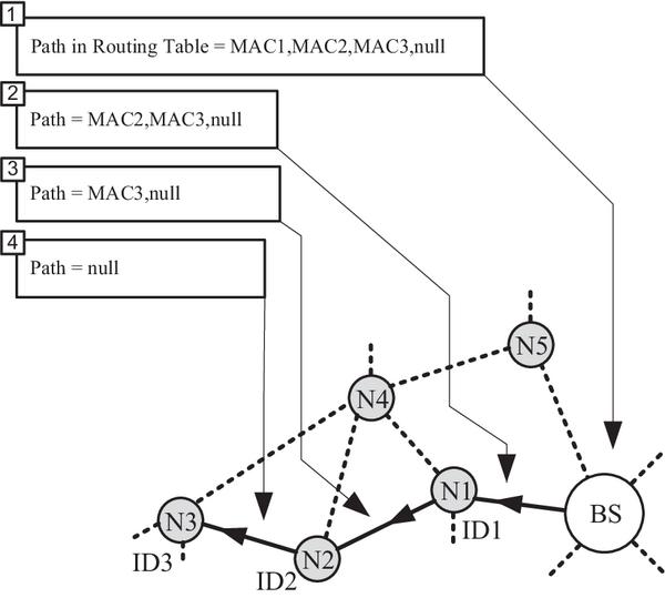
Figure 1 Value of path and length fields at different nodes on the path between BS and node N3.

Consider the situation where the BS sends a packet to sensor N3 over a pre-determined minimum cost path shown in bold in Figure 1. For this type of packets, the header includes three fields for routing: packet type, length and path. The length field specifies the length of the packet in bytes, including packet header and payload. Path information consists of the MAC address of the intermediate and destination nodes, plus a final address with a null value. The initial value of this field comes from the routing table of the BS. Each intermediate node inspects the first address of the path to determine the MAC address of the next node. Before routing the packet to the next node, each node eliminates the first address of the path field, decreases the length field, and encapsulates the packet. When the packet arrives at the destination node, the path field contains only the null value. Since most of the power consumption comes from transmission and not from packet processing, elimination of the used path information decreases the average size of the header and thus the power used for transmission.

Table 1 shows the paths from BS to nodes N2, N3 and N4 as present in the routing table of the BS used in the example. The entry for each node contains an ordered list of intermediate MAC addresses. Figure 1 shows the values of the path and length header fields as the packet passes through different nodes on the path from BS to N3. This example assumes that the packet carries a payload of 200 bytes.

Table 1 Contents of the routing table in BS for paths to nodes N2, N3 and N4 of the network in Figure 1

Num	Node	Path
…	…	…
2	ID2	MAC2, MAC1
3	ID3	MAC3, MAC2, MAC1
4	ID4	MAC4, MAC1
…	…	…

3.1.3 Unicast Messages from Sensor Nodes to Base Station

The header of unicast messages from SN to BS comprises fixed-length fields for packet type, length and ID of the source node. In the setup phase of the network (cf. Section 3.2) each node is assigned a minimum cost value, together with the ID and MAC addresses of the adjacent node on the minimum cost path to the BS (hereafter called the near-node). In the example shown in Figure 1, N2 is the near-node of N3, and N1 the near-node of N2. When SN N3 needs to send a packet to the BS, it creates a packet that includes its own ID and sends it to N2, which then passes the packet to N1. Node N1 sends the packet directly to the BS, which can use the ID field to identify the packet’s source node.

It may happen that two nodes receive a packet with the same cost value. In this case, just the near-node will process the unicast packet; all other nodes (including those with the same node cost) will discard it. This avoids the problem with equal-cost paths and the associated overhead.

3.2 Network Setup

Under SRMCF, network setup proceeds in two steps. In the first step, the cost field is set up: all nodes determine their cost values for communicating with the BS. In the second step, the BS node creates the routing table.

This step uses an approach that is similar to the minimum cost forwarding back-off algorithm [29]. Each node sets its initial cost value to ∞, except for the BS, whose cost is set to zero. Then the BS starts broadcasting its cost value. A receiver node compares its own cost value with the received cost (which includes the cost value of the sender plus the cost of the link between sender and receiver). If the received value is lower than the node’s current cost value, then the node updates its current cost to the new value, waits, and then broadcasts the new value. The waiting time increases linearly with the link cost value [9]. This process continues until all nodes set their cost values to the minimum.

The example in Figure 2 shows that node N3 has two links with the same cost (to N2 and N4), but the cost value from N2 is lower than the cost value from N4 (3 + 2 < 5 + 2). Therefore, N3 will change its own cost to 5 and designate N2 as its near-node.

The back-off algorithm decreases the number of cost advertisement messages significantly, as most of the nodes will broadcast their cost value only once.

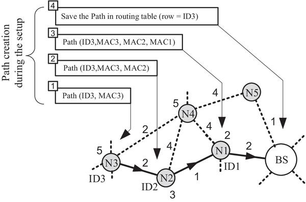
Figure 2 Adjusting the path from N3 to BS when the cost value of N3 has changed.

This algorithm cannot be used to discover optimum paths from BS to node, because the algorithm is based on setting the BS cost to zero, which is not applicable to the other nodes. Therefore, a second step has been implemented over the initial back-off concept. In the second step, the BS and the SNs cooperate in the creation of the routing table: after a node changes its cost value in the first step, it sends a packet with its ID and MAC address to its near-node, which does the same. Eventually, the BS receives a packet that includes the ID and MAC addresses of the source node, and the MAC address of all the nodes in the minimum path between source node and BS. The BS saves the ID and MAC addresses in the row of the routing table corresponding to that particular source node (cf. Section 3.1.2). Figure 2 shows this process for node N3 and Table 1 shows the value of the row corresponding to N3 (ID3 in the column “Node” of the routing table). The routing table is created without running any calculations on the BS and without any information about the network’s topology.

The procedure used in the second step is also followed during normal network operation whenever the cost value of a node changes, which may happen when a link or node failure occurs, or when a node gets a cost advertisement message with a lower value than its own previous cost.

3.3 Failure Recovery

Recovering from a link or node failure involves updating the cost value field and the corresponding minimum-cost paths stored in the BS. The method used by SRMCF is based on self-detection [30, 31] and near-node coordination [32]. For the purpose of failure recovery, each node monitors the activity of its near-node. Any message received from that neighbor will reset a watchdog timer. If there is no message within a specified time interval T_q, the node sends a query message to check the reachability of its near-node. If there is no reply, the node initiates the recovery procedure by broadcasting cost request messages periodically (up to a given amount of time defined by the variable NNQR (number of near-node query requests)).

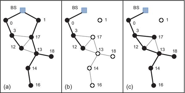
Figure 3 Failure recovery: (a) initial situation, (b) failure of node 1, (c) recovery from failure complete.

Figure 3 (a) shows part of a network with established links and corresponding minimum cost paths (bold lines). In Figure 3 (b) node 1 has failed, and nodes 17, 13, 18, 14 and 16 must find new minimum cost paths. Figure 3 (c) shows the network after recovery and Table 2 presents the cost values before and after failure. Node 13 selects node 12 as its near-node, because the correspondent new cost-value of node 17 is higher than that of node 12. In general, the cost values of nodes which are closer to the BS than the failing node are not affected.

The choice of values for the parameters T_q and NNQR depends on network density, traffic and energy consumption goals. Small values of T_q lead to faster failure detection, but increase energy consumption and decrease throughput, because more query messages are issued. Smaller values of NNQR increase the probability that a temporary absence of communication over a link (for instance, due to collisions) may be mistaken for a node failure.

The impact of the recovery procedure depends on the relative location of the SN. Nodes closer to the BS are on more minimum-cost paths than nodes on the periphery of the network. Therefore, the recovery procedure may have a large impact on the overall network performance. For outlying SNs, failure recovery only impacts locally, a behavior that enhances energy efficiency. In addition, data communication is not disrupted during recovery from failures as happens when a periodic setup phase is used with MCF [25].

Table 2 The cost value before and after a failure event

	Cost
Node	Before failure	After recovery
0	55	55
3	102	102
12	154	154
17	139	156
13	192	199
18	244	251
14	240	247
16	286	293

4 Protocol Analysis

To increase the network performance and reduce energy consumption, SRMCF was to generate less packets than MCF for transmitting the same amount of data. This section provides an analytical comparison of packets count between SRMCF and MCF. In addition, average packet header length and routing table size for SRMCF are analyzed. Later sections experimentally validate the analysis.

4.1 Packet Count

Let the set N = {n₁,n₂,...,n_m} denote the WSN nodes. If n_j is within the transmission range of n_i with reliable communication, then l_i,j denotes the link between these nodes. If the propagation channel between nodes is reciprocal and nodes are equipped with the same transmitter and receiver circuits, then l_i,j = l_j,i. In this case, let L denote the set of such reciprocal links. Then we can model the network as an undirected graph G = (N,L). In the following, we assume that G is connected. Between each pair of nodes there are many possible paths. Let P_i,j^k denote the k-th path between n_i and n_j. For random networks with n nodes, both the maximum and the average number of hops in paths between nodes increase as Θ( $\sqrt{N}$ ) [33, 34].

In order to model the communication costs, we can assign positive, additive cost functions to nodes and links. Let C_N(i) define the value of node n_i and C_L(i,j) the cost value of link l_i,j = l_j,i. It should be noted that neither C_L(i,j) nor C_L(i,j) impose additional restrictions on the cost values beyond being strictly positive and additive. So, the protocol does not impose any limitation on the cost metric and any parameter appropriate for the specific application can be chosen, e.g., hop count, node energy level or link quality. To evaluate SRMCF, we have considered hop count as the metric in the experimental implementation (Section 5). Let C_i,j^k represent the cost of sending a message from node n_j to n_i over the k-th path. Then:

C_{i, j}^{k} = \sum_{r, s \in P_{i, j}^{k}} C_{L} (r, s) + \sum_{n \in P_{i, j}^{k}} C_{N} (n) (1)

Since we are assuming reciprocal links, we have C_i,j^k = C_j,i^k, so the cost of communicating between two randomly selected nodes is independent of the direction.

Whatever the metric used to measure the cost, there is at least one path with minimum cost between two arbitrary nodes:

C_{i, j} = m i n {C_{i, j}^{k} | k \in P_{i, j}} (2)

Obviously, the minimum cost value depends on the cost metric. If energy is used as the cost metric, Equation 2 specifies a path that results in minimum energy consumption during communication; if the cost metric is the hop count, Equation 2 specifies a shortest path.

Throughput of the network

In a scenario where a sink node collects data from all other nodes, the total transport capacity or throughput of the sink is upper bounded by the maximum channel capacity W [35]. In other words, if each sensor generates an equal amount of data to send to the sink node (BS), then the maximum throughput of nodes is limited to W/N.

Let λ_n and λ_s denote, respectively, the achievable throughput of each node and the total transport capacity of sink node. If each packet must be sent r times on the path from sender to receiver node, then λ_n can be at most W/(rN). In this case, λ_s is upper bounded by:

λ_{s} \leq \frac{W}{r} . (3)

Therefore, with increasing r the maximum achievable transport capacity of all nodes, including the sink node, will decrease.

Packet count

Let T_Mⁿ and T_M^s (M stands for MCF protocol) denote the total number of packets generated by nodes other than the sink and by the sink node, respectively, when using the MCF protocol. Since the average path length increases as Θ( $\sqrt{N}$ ), the total throughput of the nodes is

T_{M}^{N} = h \sqrt{N} λ_{n} N, (4)

where h $\sqrt{N}$ denotes the average hop count and h is a positive value that depends on the network topology. then

T_{M} = T_{M}^{N} + T_{M}^{s} = h \sqrt{N} λ_{n} N + \frac{λ_{n}}{m} N, m > 1, (5)

where T_M refers the total number of packets generated when using the MCF protocol.

For the SRMCF protocol, under the same conditions, the total number of generated packets T_S (S stands for SRMCF) is:

T_{S} = h \sqrt{N} λ_{n} N + \frac{λ_{n}}{m} \sqrt{N} . (6)

From Equation (5) and (6) we have:

T_{M} = T_{S} + \frac{λ_{n}}{m} (N - h \sqrt{N}) . (7)

If the term N-h $\sqrt{N}$ is positive, Equation 7 implies that the SRMCF protocol generates fewer packets than MCF. To prove this, we determine the maximum value of h $\sqrt{N}$ . Figure 4 illustrates a line topology, which is the situation where the average hop is maximum. In this case:

\max (h \sqrt{N}) = \frac{\frac{N}{2} (N + 1)}{N} = \frac{N + 1}{2} (8)

For N > 1, it follows that

\min (N - h \sqrt{N}) = N - \frac{N + 1}{2} = \frac{N - 1}{2} > 0 (9)

Combining Equation (7) and (9) gives:

T_{M} > T_{S} (10)

Figure 4 A network topology with maximum average hop count.

Equation (10) shows that under the same conditions SRMCF generates less traffic than MCF. This means that k is smaller, leading to lower energy consumption. In addition, by Equation 3, the throughput is also higher.

4.2 Packet Header Length

SRMCF uses variable-length headers for packets from BS to pSN. In addition, the packet header length changes along the path. Let h_fix represent the packet header length (in bytes) used in packets from a SN to the BS. The header length for packets in the other direction is

h_{s i z e} = h_{f i x} + α H, (11)

where α is the length of the MAC address and H is the number of hops between the current node and the destination. The value of H is decremented as the packet progresses along the path from BS to SN. In fact, the packet header length, from node to node as it proceeds to the destination, follows an arithmetic progression with common difference {-α}. Considering the average path length (h $\sqrt{N}$ ) and the change of the packet header length, the average packet header size for SRMCF is:

\begin{array}{l} h_{a v g} \approx h_{f i x} + α (\frac{(\frac{[h \sqrt{N}]}{2}) (1 + [h \sqrt{N}])}{[h \sqrt{N}]}) \\ \approx h_{f i x} + α (\frac{1 + [h \sqrt{N}]}{2}) . (12) \end{array}

For h $\sqrt{N}$ ≫ 1 the expression becomes

h_{a v g} \approx h_{f i x} + \frac{α h \sqrt{N}}{2} (13)

Equation (13) shows that, for networks with a large number of nodes, eliminating unnecessary path information for packets from the BS to a SN almost decreases the average header length by a factor of two.

4.3 Routing Table Size

The BS keeps a routing table with all optimum paths to reach the SNs. Obviously, the size of the table depends on the number of SNs and how they are distributed in the network. Because of the variable path, there is no fixed relation between the number of nodes and the routing table size. To calculate the approximate size of the table, suppose that the average path size is (h $\sqrt{N}$ ). As mentioned in Section 3.2, the entries of the routing table includes fixed-size elements and a variable-length path. rw1 5.2 Therefore, for each row x of the table, the average table column size in bytes T_x is

T_{x} \approx T_{f i x} + α (h \sqrt{N}), (14)

where T_fix is the size of the fixed part of an entry and α is the length of the MAC address. Hence, for N nodes

T_{s i z e} \approx N (T_{f i x} + α (h \sqrt{N})), (15)

where T_size is the total routing table size in bytes. For a large number of nodes, the fixed part of the entry will be much smaller than the variable part. Then,

T_{f i x} ≪ α (h \sqrt{N}) \Rightarrow T_{s i z e} \approx Θ (N \sqrt{N}) . (16)

Equation (16) indicates that the routing table size grows in the order of N $\sqrt{N}$ , a fact that should be considered in the design of the BS. The variable entry size increases the managing complexity of the table, which must support queries by node, periodic updates of the expiration counter associated with each entry, and node insertion and deletions. If the BS has enough memory to keep a large table, then using a table with a fixed entry size will be simpler and reduce processing time. In this case, the length of each entry has to be large enough to store the biggest path. If P_max is the maximum path size (in bytes), then

T_{s i z e} = N (T_{f i x} + P_{m a x}) . (17)

Although the BS usually has more resources than the SNs, it is still useful to compress the routing table. An approach to compression is based on the idea that, if an SN is stored in the routing table, then its near-node is also registered in the table. Therefore, if a pointer that refers to the location of the near-node is used instead of the path information, the BS can generate the path through concatenation of the individual near-node path information. In this case the routing table size becomes

T_{s i z e} = N (T_{f i x} + i), (18)

where i is the index size of the routing table. This method may significantly compress the routing table.

5 Prototype Implementation and Measurements

The SRMCF was implemented on top of Contiki [36], an open-source operating system for Tiny systems, and used to manage several small networks of six TelosB motes. Table 3 lists the parameters used in the hardware implementation. The TelosB mote uses a 2.4 GHz IEEE 802.15.4 compliant RF transceiver (CC2420) [37] and a MSP430 microcontroller [38]. The energy-efficient MAC protocol of Contiki (ContikiMAC) uses a wake-up mechanism with a set of timing constraints to enable motes to control the transceivers [39].

Table 3 Parameters of prototype implementation

Parameter	Value
Mote	TelosB
Sensor nodes	6
Network area (m²)	10×10
Maximum packet length (byte)	128
Antenna reach (m)	1
Node buffer size (byte)	1024
Data rate (kbps)	250

Figure 5 Networks with different arrangement of motes: NW1—random, NW2—series, NW3—BS in the center.

Figure 5 shows three different arrangements of SNs, which were used for evaluation of the implementation. A black circle indicates the BS and gray circles represent SNs. Since the performance of the protocol also depends on the network topology, three different SN arrangements were studied. Arrangement NW2 has a line topology, in which each node has at most two neighbors. In comparison with other topologies, a line arrangement has maximum hop-count and all nodes except the last are involved in routing the packets. The node density of arrangement NW3 is higher than in the other two cases. By increasing the node density, the number of nodes inside the radio coverage of each SN increases and more transmission conflicts occur.

For the trials, SNs continuously generate traffic packets in the network layer at a fixed packet rate. To evaluate various aspects of the protocol, both of the packet size and packet rate of each SN are configurable. In addition, measurements of setup time (Table 4), energy consumption (Table 5) and failure recovery time (Table 6) were carried out as described in this section. To reduce the effects of electromagnetic interference, the measurements were made in an anechoic chamber. In order to compare the effect of the proposed protocol, the same measurements were also carried out for the MCF protocol. The presented values are the average of 20 measurements for each network.

Table 4 Measured setup times (s) for the node arrangements shown in Figure 5.

Network	MCF	SRMCF	Δ (%)
NW1	2.6	3.5	34
NW2	3.5	4.8	37
NW3	2.1	2.6	24

Table 5 Measured total energy consumption (mJ) after running for 100 s with each node generating 640 bps

	SRMCF		MCF
Network	TX	RX	TX	RX
NW1	389.88	433.26	430.92	649.89
NW2	362.52	384.71	391.93	440.73
NW3	376.2	437	424.08	679.77

Table 6 Measured failure detection and recovery times for a linear arrangement of nodes (network NW2)

Node	T_q (s)	Detection (s)	Recovery (s)
N4	22pc1	3	6
N5		3	7
N4	22pc4	9	8
N5		10	6

The setup times reported in Table 4 show that, as expected, the SRMCF protocol needs more time to complete the setup because of its additional phase for routing table generation. The failure recovery mechanism of SRMCF may also contribute to the additional setup time, because failures may also occur at this stage. Since the nodes of NW2 must perform their setup in sequence, this is the network that requires more time to complete the setup. The smallest setup time occurs for NW3 because all SNs can communicate directly with the BS. The results show that setup time decreases as the node density increases.

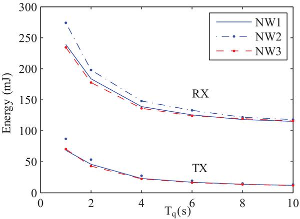
Figure 6 Energy consumption of query processing.

Table 5 shows the measured energy consumption of transmitters and receivers after running for 100 s, while each sensor generates a traffic of 640 bps. Energy consumption with SRMCF is smaller than with MCF for both transmission and reception. For transmission, SRMCF achieves 9.5% (NW1), 7.5% (NW2) and 11.3% (NW3) less energy consumption than MCF. In receiving mode the difference is more significant: 33.3% (NW1), 12.7% (NW2) and 35.7% (NW3). With MCF the receiver’s energy consumption is higher than the transmitter’s, especially when the node density is high (NW3). For these motes, the receiver module consumes slightly more energy than the transmitter. Since all receivers in the coverage area of a transmitter will receive a given packet, denser networks will exhibit higher energy consumption, specially for reception (see the values for network NW3 in Table 5). Since MCF requires more packets, the energy consumption of the networks with SRMCF will be lower. The difference is particularly significant for the receiver modules of the denser network NW3.

In order to evaluate the impact of T_q (failure query time), the three prototype networks were simulated with Cooja [40]. Figure 6 presents the simulation results of the energy consumption from near-node querying as a function of T_q for 100 s of network activity. As can be seen, the energy consumption decreases almost exponentially with increasing T_q. Network NW3 displays the lowest energy consumption, because it has the highest node density of the three. Therefore, each node has more opportunities to receive a message from its near-node and does not need to send query messages, for most of the time.

Table 6 shows the experimental results for failure recovery time in network NW2 in the absence of any data traffic. For this study, NNQR = 2 and T_q = 1 s or T_q = 4 s. To simulate failures, nodes 4 or 5 are turned off for 20 s and then turned on again. As expected, failure detection time for the case T_q = 1 is almost 4 times smaller than for T_q = 4. The recovery time is almost independent from T_q because after failure detection the node runs in idle mode. The difference in recovery time is due to the relative position of the different nodes affected by the one that has failed: If node 4 fails, five nodes will be affected, and three nodes affected for a failure at node 5 (see Figure 5 for NW2).

6 Simulation Experiments

In order to evaluate the SRMCF protocol for larger sensor networks, a large set of simulation experiments was carried out. To establish a base line for comparison, the same networks and work loads were simulated with MCF as the routing protocol. The goal is to characterize the impact of SRMCF on setup time, throughput, packet delivery, energy consumption and failure recovery time.

The operation of a routing protocol is also influenced by the MAC protocol and mote hardware. In order to increase the scope of the evaluation, both routing protocols were simulated in a setup corresponding to MICAz motes running the Berkeley-MAC (B-MAC) protocol [41], which is a CSMA-based, energy-efficient MAC protocol widely used for low-power operation, and in another setup corresponding to the TelosB motes used in the implemented prototype (cf. Section 5).

6.1 Simulation Setup

The simulations of networks with TelosB motes were done with the Cooja wireless network simulator from the Contiki project [36]; for networks with MICAz motes, the simulations were implemented in OMNet++ 4 using the MiXiM framework [42]. In both cases, the parameters for the SNs correspond to the specifications of the corresponding motes [43, 44]

Table 7 indicates the simulation parameters used for the wireless environment. Sensors are scattered randomly in a square area with the BS node located at the center. The MICAz mote is based on the ATmega128L microcontroller [45] and uses the same transceiver as the TelosB mote. The MiXiM framework includes all the code necessary to model a wireless environment including the physical layer, the radio channel, and the battery of the transceiver.

Table 7 Parameters for the simulation experiments

Parameter	Value
Mote	MICAz, TelosB
# Sensor nodes	50, 100, 200
Network area	300×300 m²
Maximum packet length	256 byte
Antenna reach	25 m
Buffer size at SN	1024 byte
Simulated time	300 s
SN data rate	250 kbps

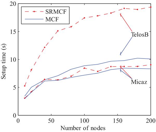
Figure 7 Network setup time for SRMCF and MCF. For SRMCF, all nodes are initialized within the setup time; for MCF, at least 90% of the nodes are initialized.

6.2 Setup time

Figure 7 shows the setup time of the network as a function of the number of sensors for networks with up to 200 nodes. At the beginning of the simulation, each sensor starts to work at a random instant in the interval between 0 s and 1 s; the BS broadcasts the first costADV message in the same interval.

The setup time depends on the number of the sensors and increases from 3 s (10 sensors) to 9 s (200 sensors) for the SRMCF protocol with MICAz motes. The MCF protocol takes less time to complete the setup. The reason, again, is that SRMCF setup is done in two steps (cf. Section 3.2), whereas the MCF protocol requires only the first. However, the SRMCF protocol requires setup to be performed only once and the difference is not high (less than 1 s for 200 sensors). Moreover, SRMCF protocol does not need to execute periodic setup phases to ensure recovery from node failures.

MICAz motes complete the setup phase slower than TelosB motes. The ContikiMAC protocol generates more packets than B-MAC, a behavior which sometimes allows the nodes to have a higher chance of receiving messages, but also increases the probability of collisions and packet losses. The SRMCF protocol with ContikiMAC (on TelosB motes) takes considerably more time to setup, mainly due to the failure recovery mechanism. When a node does not get a costADV message, it broadcasts a cost request. Collisions may also occur with the MCF protocol, causing some SNs to not receive the cost message and consequently not to turn on. For this reason, the setup time for MCF on TelosB shown in Figure 7 does not correspond to 100% of the nodes running, but instead it is obtained when the number of initialized SNs reaches 90 %, whereas the results for the SRMCF protocol on TelosB corresponds to 100 % initialized nodes. The same condition happens when the B-MAC protocol is used (MICAz motes), but a better performance is observed, because there are fewer collisions and lost packets.

6.3 Network Throughput and Packet Delivery

Figure 8 shows the total network throughput for both protocols with two different motes as a function of the data rate generated by the BS. Each sensor generates packets at a rate of 2048 bps. Networks with 50, 100 and 200 nodes were analyzed: for each size, 20 different randomly generated networks were simulated 20 times.

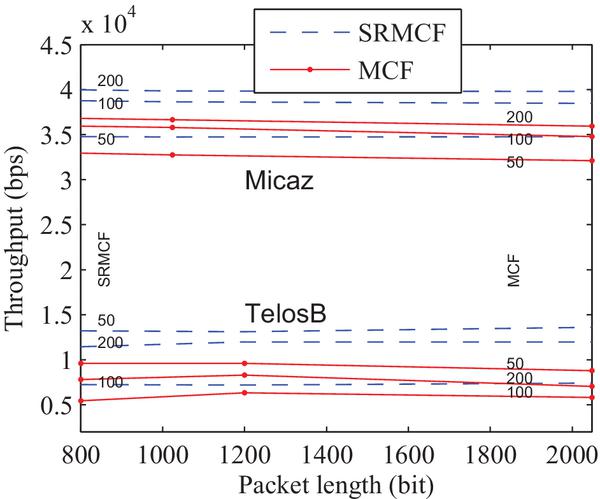
Figure 8 Throughput of the network in terms of the data rates of the packets generated by the BS (in bps).

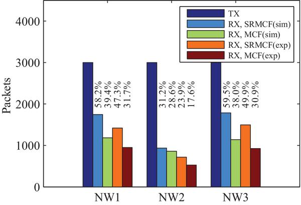
Figure 9 Simulation results for packet delivery with SRMCF and MCF protocols.

The relatively low throughput is mainly due to the MAC protocols. As Figure 8 shows, MICAz with B-MAC has amlost 3 times higher throughput than TelosB with ContikiMAC. This is caused, anew, by the higher number of packets generated by ContikiMAC, which increases the number of collisions in the network. However, the SRMCF protocol consistently achieves a higher throughput than the MCF protocol: 37.5% for 50 nodes, 33% for 100 nodes and 46% for 200 nodes. The same happens with MICAz motes, however the improvements are smaller: 5.8% for 50 nodes, 8.7% for 100 nodes, and 8.6% for 200 nodes. This is due to the fact that the SRMCF protocol is not subject to some of the problems associated with the flooding method used together with MCF, like implosion, overlapping and source blindness [1].

Figure 9 shows simulation and experimental results for packet delivery in the prototype networks. In this figure, TX is total number of generated packets, RX,x(sim) is the total number of received packet as obtained from simulation and RX,x(exp) is the total number of received packet as obtained from the actual experiment. All presented results correspond to are averages of 20 simulations or measurements, respectively. The BS and the SNs nodes generate packets periodically (5 packets/s). In total, 3000 packets are transmitted in 100 seconds.

Simulation results indicate that SRMCF protocol achieves 47%@NW1, 9.1%@NW2 and 56.6%@NW3 more packet delivery than MCF. For experimental results of packet deliver, SRMCF achieves 49%@NW1, 36%@NW2 and 61%@NW3 more than MCF. Both set of results confirm that the SRMCF protocol has better performance than MCF protocol, particularly when the node density increases (NW3). Because of less traffic with SRMCF, fewer collisions occur and packet delivery increases.

6.4 Energy Consumption

Figure 10 shows simulation results for the energy consumption of a wireless network with 50 nodes (for both MICAz and TelosB) when all nodes start to generate packets after t = 10s. The amount of traffic generated by the SNs is the same as in the throughput simulations.

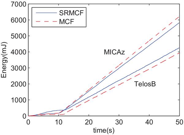
Figure 10 Energy consumption of network with 50 nodes (simulated).

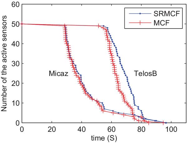
Figure 11 Number of the active nodes as a function of time.

Under the stated conditions, energy consumption increases linearly with operation time in all cases (except during the setup phase). As can be observed, after 50 s the SRMCF protocol spends 6.7% less energy with B-MAC than with ContikiMAC, due to fewer generated packets and to communication over minimum cost paths in both directions. As shown in Figure 8, for a 50-node network the throughput for SRMCF with B-MAC is 27% higher than the one for MCF. Therefore, compared to MCF, the SRMCF protocol consumes 26% less energy for the same throughput. Since power is the time derivative of energy, the figures show that power consumption is constant after the setup phase. With SRMCF total power consumption is almost 141 mW, that is 6% less than MCF (150 mW).

With ContikiMAC, the SRMCF protocol consumes 1.4% more energy than MCF, but has 43% better throughput. Therefore, in this case the SRMCF protocol consumes 29% less energy than MCF for the same throughput. The total power consumption after setup with MCF is almost 96.2 mW, that is 1.4% less than SRMCF with 97.6 mW. But as mentioned, MCF has lower throughput than SRMCF. In general, ContikiMAC results in less energy consumption than B-MAC, but leads to lower throughput.

A lower energy consumption should result in a longer network lifetime, as shown in Figure 11. This figure characterizes network lifetime by showing the number of active nodes for the SRMCF and MCF protocols. To simulate the lifetime, sensors are supplied with limited amount of energy and the number of alive and responding sensors is counted. Each wireless sensor is assumed to have a limited energy supply: a 3.3 V, 50 μAh battery for MICAz, and a capacity of 25 μAh for TelosB. The battery capacity for TelosB is reduced, because Figure 10 indicates that this platform consumes less power than MICAz.

With MCF over B-MAC, after 36.2 s, 50% of the nodes are still alive; with SRMCF, 50% of the nodes are alive after 37.8 s, a 4.4% increase in lifetime. For SRMCF with ContikiMAC, the lifetime increase is 10.6%. As mentioned before, MCF generates more packets than SRMCF. Therefore, MCF with ContikiMAC, which also generates more packets than B-MAC, consumes more energy than SRMCF with ContikiMAC and has a shorter network lifetime.

If necessary, query messages are sent periodically with time interval T_q. Small values of T_q lead to fast failure recovery, but require a large number of query messages.

6.5 Size of Packet Header and Routing Table

With SRMCF, packets generated by the BS have variable length, which depends on the number of nodes in the path between the BS and destination nodes (cf. Section 3.1.2 and 4.2). Both SRMCF and MCF have a fixed 5-byte header for packets generated by the sensor nodes. The implementation assumes that all sensors are from the same vendor. Therefore, the first three octets of MAC address, which identifies the organization that issued the address, are the same for all nodes. It is not necessary to include them in the routing path, making the packet header more compact (3 octets per each node address). Figure 12 shows the average packet header size obtained by simulating random networks with 100 to 1000 nodes. The figure also shows the calculated average header size given by Equation (13). The results confirm that the average header size only increases by a factor of 1.6 when the number of nodes increases 10 times. Using a MAC address length α = 3 and h_fix = 5, and using the simulation results form N = 100 to N = 1000, allows us to solve Equation (13) for h, obtaining h = 0.281. The average header size is then:

h_{a v g} \approx 5 + 0.281 \sqrt{N} . (19)

The dashed line in Figure 12 shows that h_avg agrees with the simulation values.

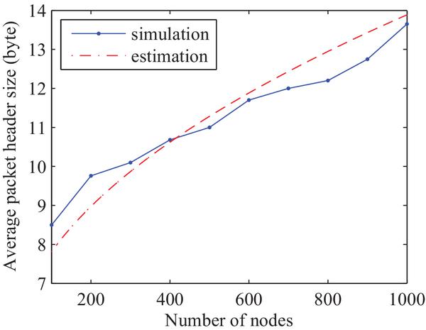
Figure 12 Average initial packet header size.

As mentioned in Section 3.1.2, each node hands over the packets generated by BS to the next node with α bytes less in the packet header. With a fixed packet header (BS to node), the header size lies between 9.5 to 24.5 bytes (for networks with 100 to 1000 nodes). Therefore, by using the method described in Section 3.1.2, the SRMCF protocol achieves a significantly smaller average packet header size. It should be noted that both protocols have a relatively small header size in relation to the overall packet size (256 bytes) used in these simulations.

The average size of routing table for the uncompressed approach characterized by Equation (15) was measured for randomly generated networks with 100 to 1000 nodes (20 samples for each network size). Figure (13) depicts those results together with the values estimated from Equation (15), (17) and (18). For this set of simulations, T_fix = 5 and the value of h obtained by interpolating the experimental results is 0.305. The simulation results agree closely with the calculated size given by Equation (15). The simpler method of using only fixed-sized entries is acceptable for small or more compact networks, but the table size becomes very significant for larger ones: for 1000 nodes, the size calculated from the average maximum path length is 34.9 kB, which is 1.49 times larger than the approach that uses variable-length entries. The use of compressed tables would allow significant savings in memory at the cost of more complex search and insertion algorithms: the table size for a 1000 node network is predicted to be 8 kB by Equation (18), a fixed value independent of network topology.

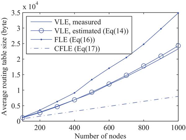
Figure 13 Average size of routing tables built using three different methods: VLE (variable-length entries), FLE (fixed-length entries), CFLE (compressed fixed-length entries).

Table 8 Comparison between the main characteristics of MCF and SRMCF

Scheme	Advantages	Drawbacks	Scalability	Mobility	Route Metric	Periodic Message Type	Robustness
MCF	Minimizes energy consumption by routing packets over paths with minimum cost.	Packets may be duplicated during routing.l Absence of failure recovery.	Good	Low	Minimum cost forwarding	Cost messages	Low
SRMCF	Minimizes energy consumption by always routing packets over paths with minimum cost and recovers from failures.	Longer back-off time.	Good	Good	Minimum cost forwarding	Cost messages	Good

6.6 Relative Comparison

All energy-efficient routing protocols discussed in Section 2 [10, 15–18] are based on minimum cost routing and minimize routing cost for communication in the direction from sensor nodes to BS, whereas routing performance in SRMCF is optimized in both directions (from nodes to BS and vice-versa). rw.3, rw.6 Table 8 compares the MCF and SRMCF protocols. In comparison with the other protocols, SRMCF shows good performance in terms of scalability, mobility and robustness. Because of the absence of any recovery method in MCF and the other aforementioned protocols, these protocols are not able to recover from topology changes in networks with mobile nodes, whereas, with SRMCF, nodes find another minimum cost path whenever their location changes.

7 Conclusion

The adoption of source-based routing in SRMCF leads to an improvement of the performance over the MCF protocol. SRMCF is energy-efficient, reactive and does not require routing tables at every sensor node. Unlike MCF, it applies the minimum cost forwarding method in both directions. The absence of link and node failure control in MCF hampers its use in practical applications. The proposed failure recovery mechanism for SRMCF solves this limitation without affecting data communications.

Both the theoretical analysis and simulation experiments described in this work show that SRMCF has both higher throughput and smaller energy consumption than MCF. Packet delivery and energy consumption are also shown to improve with the use of SRMCF. The impact of the MAC layer was investigated through simulations with the ContikiMAC and B-MAC protocols. The simulations indicate better performance of SRMCF when used together with ContikiMAC.

Based on experimental and simulation results, it can be concluded that minimum cost forwarding, failure recovery mechanism, absence of equal cost paths problem and improved performance make SRMCF a good candidate for energy-efficient, practical wireless sensor applications.

References

[1] I. F. Akyildiz, W. Su, Y. Sankarasubramaniam, and E. Cayirci, “A survey on sensor networks,” vol. 40, pp. 102–114, Aug. 2002.

[2] M. Ilyas and I. Mahgoub, Handbook of Sensor Networks: Compact Wireless and Wired Sensing Systems. CRC Press LLC, USA, 2005.

[3] X. Li, Wireless Ad Hoc and Sensor Networks, Theory and Applications. Cambridge University Press, USA, 2008.

[4] W. Dargie and C. Poellabauer, Fundamentals of Wireless Sensor Networks: Theory and Practice. Wiley, 2010.

[5] C. Ma and M. Ma, “Data-centric energy efficient scheduling for densely deployed sensor networks,” in IEEE Intl. Conf. on Communications, pp. 3652–3656, 2004.

[6] F. Derogarian, J. C. Ferreira, and V. M. G. Tavares, “A routing protocol for WSN based on the implemention of source routing for minumum cost forwarding method,” in Fifth Intl. Conf. on Sensor Tech. Appl. (SENSORCOMM2011), Aug. 2011.

[7] Y. Zhong and D. Yuan, “Dynamic source routing protocol for wireless ad hoc networks in special scenario using location information,” in ICCT Intl. Conf. on Communication Technology Proceedings, vol. 2, pp. 1287–1290, 2003.

[8] J.-E. Garcia, A. Kallel, K. Kyamakya, K. Jobmann, J.-C. Cano, and P. Manzoni, “A novel DSR-based energy-efficient routing algorithm for mobile ad-hoc networks,” in 58th IEEE Intl. Conf. on Vehicular Technology, vol. 5, pp. 2849 – 2854, Oct. 2003.

[9] F. Ye, A. Chen, S. Lu, and L. Zhang, “A scalable solution to minimum cost forwarding in large sensor networks,” in 10th Intl. Conf. on Computer Communications and Networks, pp. 304–309, 2001.

[10] T. V. Padmavthy, G. Divya, and T. R. Jayashree, “Extending network lifetime in wireless sensor networks using modified minimum cost forwarding protocol-mmcfp,” in 5th Intl. Conf. on Wireless Communications, Networking and Mobile Computing, WiCom’09., pp. 1–4, 2009.

[11] B. Baranidharan and B. Shanthi, “A survey on energy efficient protocols for wireless sensor networks,” vol. 11, pp. 35–40, Dec. 2010.

[12] W. R. Heinzelman, A. Chandrakasan, and H. Balakrishnan, “Energy-efficient communication protocol for wireless microsensor networks,” in 33rd Intl. Conf. in System Sciences, 2000.

[13] S. Lindsey and C. S. Raghavendra, “PEGASIS: Power-efficient gathering in sensor information systems,” in IEEE Aerospace Conf. Proceedings, vol. 3, pp. 1125–1130, 2002.

[14] Z. Zhang and F. Yu, “Performance analysis of cluster-based and tree-based routing protocols for wireless sensor networks,” in Intl. Conf. on Communications and Mobile Computing (CMC), vol. 1, pp. 418–422, Apr. 2010.

[15] W. Hao-ran, “Low-power routing protocol of data aggregation-based for wireless sensor networks,” in 2nd Intl. Conf. on Industrial and Information Systems (IIS), vol. 1, pp. 327–329, July 2010.

[16] S. Cai, S. Zhang, G. Wu, Y. Dong, and T. Znati, “Minimum cost opportunistic routing with intra-session network coding,” in IEEE Intl. Conf. on Communications (ICC), pp. 502–507, June 2014.

[17] S. O. Elbassiouny and A. M. Hassan, “Energy-efficient routing technique for wireless sensor networks under energy constraints,” in Intl. Wireless Communications and Mobile Computing Conf. (IWCMC), pp. 647–652, Aug 2015.

[18] E. Baby and K. B. Senthilkumar, “Hybrid multi-rate multipath routing (hmmr) protocol,” in 3rd Intl. Conf. on Advanced Computing and Communication Systems (ICACCS), vol. 01, pp. 1–8, Jan 2016.

[19] J. Zhou, H. Xu, Z. Qin, Y. Peng, and C. Lei, “Ad hoc on-demand multipath distance vector routing protocol based on node state,” vol. 5, pp. 408–413, September 2013.

[20] W. Guo, W. Zhang, and G. Lu, “Pegasis protocol in wireless sensor network based on an improved ant colony algorithm,” in Second Intl. Workshop on Education Technology and Computer Science (ETCS), vol. 3, pp. 64–67, March 2010.

[21] S. Pleisch, M. Balakrishnan, K. Birman, and R. van Renesse, “Mistral: Efficient flooding in mobile ad-hoc networks,” in 7th ACM Intl. symposium on Mobile ad hoc networking and computing, pp. 1–12, 2006.

[22] M. Ayash, M. Mikki, and Y. Kangbin, “Improved aodv routing protocol to cope with high overhead in high mobility manets,” in Sixth Intl. Conf. on Innovative Mobile and Internet Services in Ubiquitous Computing (IMIS), pp. 244–251, July 2012.

[23] S. J. Lee, W. Su, and M. Gerla, “On-demand multicast routing protocol in multihop wireless mobile networks,” vol. 7, pp. 441–453, Dec. 2002.

[24] M. Patil and R. Biradar, “A survey on routing protocols in wireless sensor networks,” in 18th IEEE Intl. Conf. on Networks (ICON), pp. 86–91, Dec 2012.

[25] D. W. Henderson and S. Torn, “Verification of the minimum cost forwarding protocol for wireless sensor networks,” in IEEE Conf. on Emerging Technologies and Factory Automation, ETFA06, pp. 194–201, 2006.

[26] R. Draves, J. Padhye, and B. Zill, “Routing in multi-radio, multi-hop wireless mesh networks,” in 10th ACM Intl. Conf. on Mobile computing and networking, MobiCom ’04, pp. 114–128, 2004.

[27] S. Ahmad, I. Awan, A. Waqqas, and B. Ahmad, “Performance analysis of DSR and extended DSR protocols,” in 2nd Asia Intl. Conf. on Modeling Simulation, pp. 191–196, May 2008.

[28] F. Ye and R. Pan, “A survey of addressing algorithms for wireless sensor networks,” in 5th Intl. Conf. on Wireless Communications, Networking and Mobile Computing, WiCom ’09., pp. 1–7, 2009.

[29] F. Ye, A. Chen, S. Lu, and L. Zhang, “A scalable solution to minimum cost forwarding in large sensor networks,” in 10th Intl. Conf. on Comput. Comm. and Networks, 2001, pp. 304–309, 2001.

[30] M. Asim, H. Mokhtar, and M. Merabti, “A fault management architecture for wireless sensor network,” in Intl. Conf. on Wireless Communications and Mobile Computing, IWCMC08, pp. 779–785, 2008.

[31] P. Yu, S. Jia, and P. X. Yuan, “A self detection technique in fault management in WSN,” in Intl. Conf. on Instrumentation and Measurement Technology, I2MTC, pp. 1–4, 2011.

[32] A. Sheth, C. Hartung, and R. Han, “A decentralized fault diagnosis system for wireless sensor networks,” in IEEE Intl. Conf. on Mobile Adhoc and Sensor Systems, pp. 194–196, 2005.

[33] L. Alazzawi, A. Elkateeb, and A. Ramesh, “Scalability analysis for wireless sensor networks routing protocols,” in 22nd Intl. Conf. on Advanced Information Networking and Applications – Workshops, AINAW 2008., pp. 139 –144, march 2008.

[34] C. Santivanez, B. McDonald, I. Stavrakakis, and R. Ramanathan, “On the scalability of ad hoc routing protocols,” in 21th IEEE Intl. Conf. on Computer and Communications Societies, INFOCOM, vol. 3, pp. 1688–1697, 2002.

[35] D. Marco, E. J. Duarte-Melo, M. Liu, and D. L. Neuhoff, “On the many-to-one transport capacity of a dense wireless sensor network and the compressibility of its data,” in 2nd Intl. Conf. on Information processing in sensor networks, IPSN’03, (Berlin, Heidelberg), pp. 1–16, 2003.

[36] Contiki OS, The Open Source OS for the Internet of Things, Available in http://www.contiki-os.org/, Jan. 2016.

[37] Texas Instruments, CC2420,IEEE 802.15.4 compliant RF transceiver, Available in http://www.ti.com/product/CC2420, Jan. 2016.

[38] Texas Instruments, MSP430, Ultra low power microcontroller, Available in http://www.ti.com/lsds/ti/microcontrollers_16-bit_32-bit/msp/overview.page, Jan. 2016.

[39] J. Ko, N. Tsiftesa, A. Dunkels, and A. Terzis, “Pragmatic low-power interoperability: Contikimac vs tinyos lpl,,” in 9th IEEE Communications Society Conf. on Sensor, Mesh and Ad Hoc Communications and Networks, SECON, pp. 94–96, 2012.

[40] F. Osterlind, A. Dunkels, J. Eriksson, N. Finne, and T. Voigt, “Cross-level sensor network simulation with COOJA,” in 31st IEEE Conf. on Local Computer Networks, pp. 641–648, Nov. 2006.

[41] C. Cano, B. Bellalta, A. Sfairopoulou, and J. Barcelo, “A low power listening MAC with scheduled wake up after transmissions for wsns,” vol. 13, pp. 221–223, April 2009.

[42] A. Köpke, M. Swigulski, K. Wessel, D. Willkomm, P. T. K. Haneveld, T. E. V. Parker, O. W. Visser, H. S. Lichte, and S. Valentin, “Simulating wireless and mobile networks in OMNeT++: the MiXiM vision,” in 1st Intl. Conf. Sim. Tools and Tech. for Comm., Networks and Syst. & Workshops, (ICST, Brussels, Belgium, Belgium), pp. 71:1–71:8, 2008.

[43] Crossbow Technology, Micaz: 2.4Ghz Mote, Available in http://www.openautomation.net/uploadsproductos/micaz_datasheet.pdf, Jan. 2016.

[44] Crossbow Technology, TELOSB: 2.4Ghz Mote, Available in http:// www.memsic.com/userfiles/files/Datasheets/WSN/telosb_datasheet.pdf, Jan. 2016.

[45] Atmel, 8-bit Atmel Microcontroller with 128 KBytes In-System Programmable Flash, Available in http://www.atmel.com//journal_article_html/html_images/jmm/Vol144/ doc2467.pdf, Jan. 2016.

Biographies

images

Fardin Derogarian Miyandoab received B.S. in communication engineering from Tabriz University in 1997 and M.S. in electronic engineering from Urmia University in 2003 and PhD in telecommunication from Porto University in 2015. His thesis focused on wearable systems and body area networks. He was lecturer at Telecommunication Company of West Azerbaijan from 2003 to 2009 and at Urmia Azad University from 2007 to 2009. From 2015, he has joined to Radio Systems group in Instituto de Telecomunicações as a postdoctoral fellow. His current research interests include telecommunication, integrated circuits, wireless sensor networks, body area network, wearable health systems, cognitive radios, energy harvesting, and mobile networks.

images

João Canas Ferreira received the Ph.D. degree in Electrical and Computer Engineering from the University of Porto (Portugal) in 2001. He is currently an Associate Professor (with tenure) with the Faculty of Engineering, University of Porto, and a senior researcher at INESC TEC, where he conducts research in dynamically reconfigurable systems, application-specific digital system architectures, sensor networks and flexible hardware for cognitive radio. He has authored or co-authored more than 80 papers in international conferences and journals. He has participated in numerous European and national research projects. He has been active in the organization of several conferences in the area of digital systems design and is handling editor for Microprocessors and Microsystems. He is senior member of IEEE, and a member of ACM and Euromicro.

images

Vítor M. Grade Tavares received the Licenciatura and M.S. degrees from the University of Aveiro, Portugal, in 1991 and 1994, respectively, and the Ph.D. degree from the Computational NeuroEngineering Laboratory, University of Florida, Gainesville, USA, in 2001, all in electrical engineering. In 1999, he joined the University of Porto, Portugal, as an Invited Assistant, where he has been an Assistant Professor since 2002. In 2010 he was a Visiting Professor at Carnegie Mellon University, USA. He is also a Senior Researcher at the Instituto de Engenharia de Sistemas e Computadores, Tecnologia e Ciência, Porto. His research interests include low-power, mixed-signal and neuromorphic integrated-chip design and biomimetic computing, CMOS RF integrated circuit design for wireless sensor networks, and transparent electronics.