EEHRP: Energy Efficient Hybrid Routing Protocol for Wireless Sensor Networks
Nandkumar Kulkarni1,*, Dnyaneshwar Mantri1, Neeli Rashmi Prasad2 and Ramjee Prasad3
1Sinhgad Institutes, Pune, India
2International Technological University (ITU), San Jose, USA
3Department of Business Development and Technology, Aarhus University, Aarhus, Herning, Denmark
E-mail: npkulkarni.pune@gmail.com; dsmantri@gmail.com; neeli.prasad@ieee.org; ramjee@btech.au.dk
*Corresponding Author
Received 18 September 2020; Accepted 30 November 2020; Publication 26 January 2021
Abstract
With Multi-Objective Optimization (MOO) mechanisms, many practical scenarios are imitated in Wireless Sensor Networks (WSNs). In MOO numerous desirable conflicting or non-conflicting objectives contend with one another and the decision has to be done among multiple available solutions. Based on the type of situation, Programme, and issue to be solved, the MOO problem has varied solutions. The solution chosen is a tradeoff solution on several occasions. In WSN, it is possible to identify MOO issues and associated solutions based on network architecture, node deployment, MAC strategies, routing, data aggregation, node mobility, etc. In this context, the paper proposes mobility aware, competent; delay tolerant Energy Efficient Hybrid Routing Protocol (EEHRP). Optimizing several metrics to pick the best route from the source to the target node is the cornerstone of the EEHRP. Multi-Objective optimization from optimization theory is a NP-hard problem. EEHRP seeks to obtain a Pareto optimal solution for the section of best MOO-based route under sensor node. The simulation results demonstrate that, relative to state-of-the-art solutions, EEHRP is efficient in terms of energy, throughput, delay, control- and routing-overheads. Furthermore, the paper investigates statistical significance of the findings obtained across confidence intervals. To prove EEHRP’s competence, a confidential interval of 95% is inserted into the simulation results obtained to represent margin of error around the estimated points. The on-hand state-of-art solutions and the propensity of the research fraternity in relation to MOO are also analyzed in this paper.
Keywords: Energy consumption, multi-objective-optimization, routing, wireless sensor network (WSN).
1 Introduction
Through value-added WSN application areas, the information handling criteria have need of careful attention to lessen the energy consumption, and latency in communication. Nodes that are utilized to collect as well as to communicate optimally routed information to the sink, have limited assets for instance energy, bandwidth, processing speed as well as memory for storage. The lifetime of WSN is governed by the energy consumption of the nodes for the duration of communication of aggregated information packets to destination than during computation and sensing. This is for the reason that the radio inside the sensor nodes utilize more energy during transmission as well as reception. In WSNs, it is very hard to alter the energy source of sensor node, unlike the customary wireless networks. This is the most differentiating characteristic of WSNs, the node’s energy depletion consequence is partitioning of network and eventually failure of the network. IOT systems, where enormous information is obtained from various sources, need secure information transmission through optimal route to destination. For an efficient routing in WSN, proper balance needs to be achieved amongst available multiple -paths as well as -nodes. The effort to choose the efficient route need to consider Single-hop or multi-hop communication, transmission-, propagation- delay, energy depletion, the number of packets –transmitted, –received, in addition the number of nodes encompassing transmission must be considered for optimal route selection [1].
WSNs are different than the customary ad-hoc and cellular network. First of all, WSNs have enormous number of sensors organized in addition it is extremely hard to allocate globally unique address to every node, so dealing with data rather than identifying it is important. Second, with the limited resources like energy, memory in addition to bandwidth, the nodes are utilized for sensing plus communication. Third, due to energy depletion, and node mobility the overheads escalates reducing network lifespan. Fourth, WSN is specific to the application and aggregation of data collected will be based on common phenomenon [2, 3].
As a result of multipath data dissemination, as soon as a receiver node take delivery of more than one packet concurrently, collision occurs and that is the major cause of energy depletion and delay in data delivery. Collided packets are discarded by the recipient and energy depletion and packet delivery time increases due to retransmission of these packets from the sender. Since the packets generated by various nodes are of different in numbers, they are sent to BS in the dissimilar time slot [2–4].
Duty-cycled scheduling and synchronization of routes may be the various techniques to decrease energy depletion. Countless thought-provoking concerns such as Node location, Energy concerns, Data transfer model, Node/link heterogeneity, Fault endurance, Scalability, Transmission process, Association, Exposure, Data gathering, govern the strategies of routing in WSNs. In this context, demands for the development of lightweight multi-objective protocol are increasing. The prime goal of multi-objective protocol is to enhance data management capability, in addition to finding the effective route in terms of condensed -latency, -energy depletion, plus -routing overheads [5–13]. With increasing demand for energy saving applications and decreased communication latency, Multi–objective routing is a promising technique to achieve better QoS in WSNs.
The focus of paper is elaborated with different sections as; Section 2 presents an overview of related works focusing on the requirements of Multi-objective routing protocols in WSN-IOT. Information on the motivation, assumptions, system model of proposed EEHRP is given in Section 3. Section 4 describes energy model of EEHRP. EEHRP mobility model is described in Section 5. Simulation setup and results are discussed in Section 6 and the paper is finally summarized in Section 7 with a fruitful conclusion and future work.
2 Related Work
Many researchers have suggested numerous multi-objective routing protocols banking on number of requirements, design issues as well as applications to escalate energy efficiency nevertheless, no routing protocol is ideal [4]. On the basis of location, layout and working ways and means diverse routing schemes proposed in [14] by way of different addressing scheme. A lightweight routing protocol (LNDIR) is proposed in [15] that manoeuvres on the state of nodes radio. To achieve minimal latency with improved energy efficiency, it changes the duty cycle when scheduling the activities of nodes in the network. In [16], author put forwards a way of reducing the communication delays and overheads amongst source node as well as destination by way of crowded network. The routing paths are often taken into consideration when the data is transmitted. Multi-Objective Decomposition based Evolutionary Algorithm (MOEA/D) [17] is envisioned to resolve the problem of the energy preservation, by means of precise awareness around problem specific facts in addition to Euclidean distance amongst the weight vectors. AACOCM [18] recommends a multi-objective model for route optimization banking on energy consumption, network latency, besides packet loss rate. AACOCM attempts to lessen energy, delay, and PLR. The functioning of AACOCM depends on ordinary-, greedy-, unusual- ant nodes. The routing tree is constructed here; data is transmitted plus response from destination is taken. As convergence ratio is greater, the large-scale network is optimal for AACOCM [19]. Proposes scalable, multi-objective framework focused on the native awareness of every single node in which Source_id, Unicast/Multicast, LRC and intend define routing. By avoiding low-energy route, hazardous areas, LRC and RO is removed. Simple Hybrid Routing Protocol (SHRP) [20] chooses the finest route built on the metrics such as hop-count, LQI, and Residual-energy. In SHRP, if either there is a shift in the value of the metrics or periodically, the route is changed. SHRP usually prefers a route with smaller hop-count and greater residual-energy. Using LQI, SHRP tackles the easily broken link and dead neighbor problem. DyMORA [21] is an extension of SHRP, which is constructed on the Hierarchical-Routing-Algorithm (HRA) as well as multi-objective hybrid strategy. To choose Pareto’s optimal path, DyMORA makes smaller number of assessments. It demands for additional processing time owing to the MO mechanism.
3 EEHRP: Energy Efficient Hybrid Routing Protocol
3.1 Motivation
Centered around a single metric, most traditional routing protocols direct the data. They follow a strategy where a threshold for a metric is defined as a locus. Directing data from source to base station is obligatory for a fraction of the total number of nodes, besides other nodes are in sleep mode. This mechanism causes the energy concerning the energetic nodes to rapidly deplete. These energetic nodes will dissipate their energy in due course in addition they will become dead. A partitioned network would end this phenomenon. EEHRP uses route selection based on several metrics to mitigate this problem. Multiple metrics optimization at the same time benefits to align the energy concerning different nodes in the network by way of diverse paths available from source to base station. WSN’s MOO problem is demonstrated in Figure 1 where prospects of Input, Output, Constraint and Objective section are specified. In order to optimize PDR, Throughput, Network lifetime, etc. in addition to picking up the best route commencing source to sink, EEHRP utilizes Control Overhead,
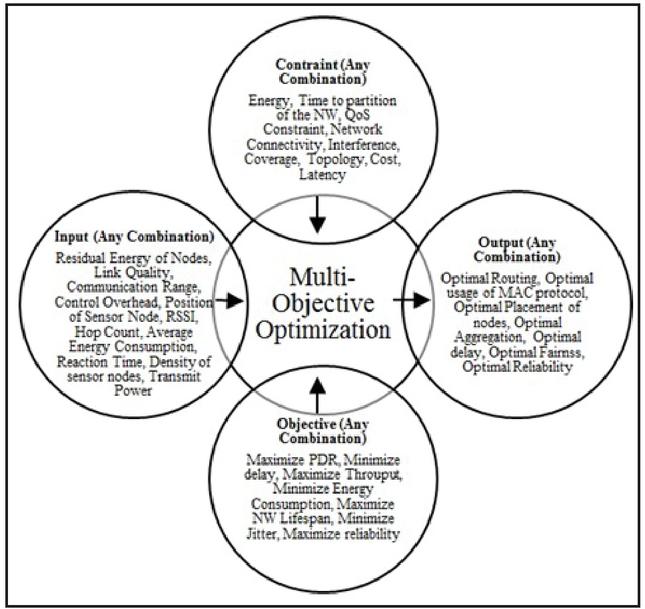
Figure 1 MOO problem in WSN.
HOP Count LQI, Average Energy Consumption, and Reaction Time from the input segment with the restriction of energy consumption, latency, time to partition besides QoS. EEHRP evolution for instance is shown in Figure 2. Low Layer-, Route Selection-, as well as Cost Control-components utilized besides the challenges embarked in EEHRP are depicted in Figure 2.
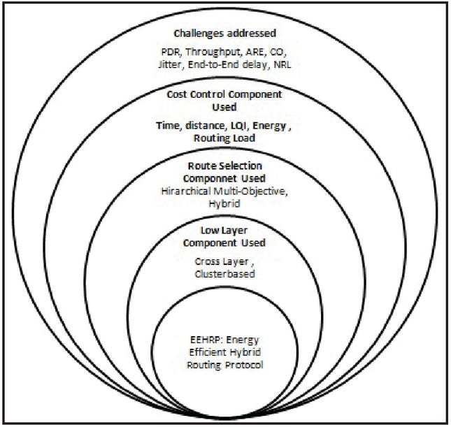
Figure 2 Evolution of EEHRP.
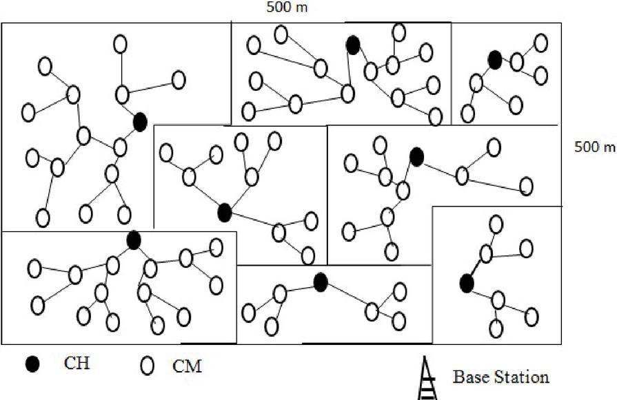
Figure 3 A clustered wireless sensor network.
3.2 Assumptions, System Model of EEHRP
3.2.1 Assumptions to implement EEHRP
Assumptions of Nodes
• Altogether nodes are identical.
• Nodes have no room for GPS.
• There’s a UID for every single node.
• The Base Station (BS), CHs are immobile besides a small number of nodes (20% of the over-all nodes) are movable.
Assumptions of Network
• The network has only one BS.
• The network is distributed amongst diverse clusters; with every cluster having a CH in addition to CM.
• The CH election is built around the multi-objective function’s end result.
• A BHT is formed inside the clusters by every single CM. The root of the BHT is designated for instance as CH.
• Inside cluster, for single hop communication amongst nodes, bidirectional links are utilized.
3.2.2 System Model of EEHRP
The whole target zone is fragmented into miniature clusters. Every single cluster has Cluster-Head (CH) as well as Cluster-Member (CM). The sensor nodes are positioned arbitrarily in the interior of targeted zone in addition they are steady. In concern with initial energy, all the sensor nodes are identical. In the targeted zone, the CMs held responsibility for recognizing the events. In electing the CH, every single CM participates. The CMs communicate solely with the CH of that cluster or the CMs of the similar cluster. They are not permitted to communicate directly to CMs or even CHs from the opposite cluster. The CHs have a second level of hierarchy. The CHs are able to communicate to another cluster’s CHs. A high-energy node arranged far from the topographic point may be the Base Station (BS). The CM, CHs plus the sink node are immobile. At the outset, the density of sensor nodes in the interior of the topographic point is enormous for the reason that it helps for the cluster based routing.
As a graph (G), WSN is demonstrated in Figure 3. In G the vertices of the graph are modelled as sensor nodes. The graph G (V, E) where V V…..V is set of vertices, and E = (n, n) V X V | i j is a set of edges amongst v and v. Intra- and Inter-cluster conversation is regarded as diverse hierarchy levels. CMs inside the cluster designate a CH banking on a fitness function cited in Section 3 at the first level in the hierarchy. Rationally, The CMs will assemble themselves resembling a BHT. As we move up in the tree from leaf- to root-node in the BHT fitness function’s cost escalates. BHT’s root node will turn out to be CH. For every cluster, the process is reiterated. The position of CH is shuffled amongst the different CMs after consecutive rounds of communication, to preserve equilibrium of energy within the entire network. All the CHs will be organized into BHT at the second layer of the hierarchy then the process is reiterated in lieu of intra-cluster communication. The accumulated data will be forwarded by the designated CH to the BS.
3.3 EEHRP Flowchart
The EEHRP algorithm functions in four phases as shown in Figure 4
Phase I-Intra-Cluster Binary Heap Tree (BHT) formation
Phase II-Intra-Cluster communication and data transfer
Phase III-Inter-Cluster Binary Heap Tree formation
Phase IV-Inter-cluster communication and data transfer
3.3.1 Phase I – Intra-cluster binary heap tree formation
From the first step as revealed in Figure 3, all the sensor nodes are positioned haphazardly in the target zone. The nodes are grouped into a multiple cluster. At this juncture, the hypothesis is that number of clusters contained by the target zone in addition to Cluster development is a preceding step to the functioning of EEHRP mechanism. This step is rendering to the clustering algorithm developed in [19]. Based on a fitness function resulting from multiple metrics such as energy, overhead, response time LQI, as well as hop count, the proposed EEHRP seeks to find the optimal route. The fitness function utilized is mentioned in the subsequent equation [13].
| (1) |
Where , , , , are weighing factors.
A cost function will be determined by means of Equation (1) by each and every cluster member inside the cluster. The CH shall be chosen in the first round on the basis of highest -residual energy, -number of neighbour nodes having one-hop connectivity as well as the minimum distance to sink [14, 20]. The threshold for the node to turn out to be CH is reviewed in [15] by means of above mentioned considerations. The BHT root will turn out to be the CH in addition all other nodes will logically organize themselves to form a BHT.
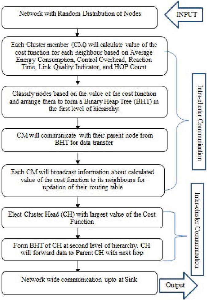
Figure 4 Flowchart of EEHRP.
3.3.2 Phase II – Intra-cluster communication and data transfer
All the child nodes will communicate the sensed information to their immediate (logical) parent in addition the parents will communicate to their parents then the process is reiterated until the information finally collected by the root node. The leaf nodes of the BST (This is a logical arrangement) will be CMs having smaller calculated value in accordance with Equation (1).
3.3.3 Phase III – Inter-cluster binary heap tree formation
The procedure used in EEHRP is recurrence in nature. All the CHs from Phase I will compute cost according to the fitness function talked about in Equation (1). The CH is elected for the second round in accordance with highest -residual energy, -number of neighbour nodes, along with one-hop connectivity besides having minimum distance to sink. The root of BHT will be elected as CH, at that moment all other nodes will logically position themselves to form a BHT.
3.3.4 Phase IV – Inter-cluster communication and data transfer
All the CHs those are child nodes will transfer the aggregated information as of different clusters in the Phase II to their direct (logical) parent in addition to this the parents will transfer information to their parents. This process is reiterated until the information finally collected by the root node. The aggregated data will be communicated to the sink by CH, which is a root of BHT in this round. The leaf nodes of the BST (This is a logical arrangement) will be CMs having smaller calculated value in accordance with Equation (1).
4 Equations of Energy-Efficiency of EEHRP
Each node is non-rechargeable and has the opening energy of E0. Energy depletion while transferring a packet commencing with ith node to jth node uses a free-space in addition to multi-path fading model banking on the distance amongst source as well as target. Depending upon distance and whether a node is a child or parent node in BHT the energy depletion varies for all packet of size Ps.
If the child node transfers Ps bytes of data, then the energy depletion is specified as: (Ref. Equation (2) to (6)) [22]
| (2) | ||
| (3) |
Where, is electronic- energy positioned around coding, distribution, modulating, filtering and amplification, is the distance amongst ith and jth node. When the jth node takes the delivery of the packet of size Ps the energy dissipation is specified as:
| (4) |
The energy cost of all nodes is corrected after every transfer or reception of packet of size Ps.
| (5) | ||
| (6) |
The process of information transfer as well as energy cost alteration is reiterated till every node is dead.
5 Equations of Mobility-Awareness of EEHRP
In EEHRP, movable nodes are well thought-out to move alongside a one-dimensional zone, as well as exponentially disseminating the pause-time. EEHRP utilizes the mobility Random-Way-Point (RWP) model. In this model, the endpoint, travel speed and not the end-users control interval of movement of nodes. The succeeding segment exemplifies thru mathematical equations how the mobile state propagation goes forward over time.
Notations
• [a1, au] – Area where the sensor node can travel
• – Exponential distributed pause time
• d – Destination Point
• r (d) – Random Distribution
• Vmax – Upper bounded Speed
• K (t) – Instantaneous State of the node
• Ø(t) – Instantaneous Phase of the node either Move or Pause
• A (t) – Instantaneous Position belongs to [a1, au]
• V (t) – Current Speed belongs to in case
• D(t) – Current destination belongs to [a1, au].
• P (a, v, d, t) – Cumulative probability at time t in case
• Q (a, t) – Cumulative probability at time t in case at position
If the mobile node travels in the target zone, then first they pick out ‘d’ according to r(d). Then they pick the speed allowing to the distribution for . fit in to the interval . Markov-Process, where is characterized by , regulates the dynamism of the mobile node. The probability at time (t) of a mobile node is (Ref. Equation (7)–(15)) [23]
| (7) | ||
| (8) |
Introducing the densities
| (9) | ||
| (10) |
Subsequent pair of equations can be obtained
| (11) | ||
| (12) |
Boundary Situation
It depicts the chance of a mobile node hitting the boundary is null
| (13) | ||
| (14) |
The initial situation
| (15) |
which is an appropriate pdf for mobile node’s original position, speed, and endpoint. The procedure for building neighborhood relationship is given in Figure 4.
Table 1 Simulation parameters
| Wireless Physical | |
| Network interface type | Wireless Physical |
| Radio propagation model | Two-Ray Ground |
| Antenna type | Omni-directional Antenna |
| Channel type | Wireless Channel |
| Link Layer | |
| Interface queue | Priority Queue |
| Buffer size ( ifqLen) | 50 |
| MAC | 802.11 |
| Routing protocol | EEHRP, DyMORA, SHRP |
| Energy Model | |
| Initial energy (Joule) | 20 |
| Radio Model | TR3000 |
| Idle power (mW) | 13.5 |
| Receiving power (mW) | 13.5 |
| Transmission power (mW) | 24.75 |
| Sleep Power (W) | 15 |
| Node Placement | |
| Number of nodes | 50, 60, 70, 80, 90 and 100 |
| Number of sink | 1 |
| Placement of the Sink | Bottom right corner of the simulation area |
| Placement of nodes | Nodes are placed randomly in the given area |
| Node placement | Random |
| Number of simulation runs | 20 |
| Miscellaneous Parameters | |
| Area(m) | 500 * 500 |
| Simulation time (s) | 2000 |
| Packet size (bytes) | 64 |
| Hello Interval (s) | 5 |
| CH Election Interval (s) | 20 |
| Packet Interval (s) | 0.2 |
| Mobility | 20% nodes are mobile |
6 Simulation and Result Analysis of EEHRP
The Network Simulator (ns2.34) is used to accomplish simulation. The simulation objective is to perceive QoS parameters as well as to equate EEHRP, SHRP, and DyMORA by means of Packet-Delivery-Ratio (PDR), Throughput, Average-Residual-Energy (ARE), End-to-End Delay, Control-Overhead (CO), Jitter, and Normalized-Routing-Load (NRL) in order to authenticate the performance of EEHRP with the simulation parameters stated in Table 1 [13].
6.1 Confidence Interval
A confidence interval deals with a range of values which is likely to enclose the population parameter of concern. One is quite sure that precise value lies in it.
6.1.1 Calculating the Confidence Interval
Notations
• n – The number of observations (sample size)
• x Total population (data values)
• – Sample mean
• – Population mean
• – Sample standard deviation
• z – Confidence coefficient
• – Confidence level
• – Margin of error
Assumption
Instead of using the standard deviation of the entire population (data values), the standard deviation for the sample is considered as the simulation results have enough observations.
Following steps are involved in calculating the Confidence Interval
• Step 1: Decide the phenomenon to be tested.
Through simulation, the paper investigates the accuracy of EEHRP, SHRP, and DyMORA when the data packets are routed from source to destination (i.e. accuracy in routing).
• Step 2: Select a sample from your chosen population.
This step is used to gather data for testing the hypothesis. The simulation is carried out for number of nodes from 50 to 100 in step of 10. The nodes are randomly distributed in the target area of 500 500 meter. For each scenario the simulation is repeated 20 times (simulation run) and the average value of 20 iterations is taken into account for finding the values of the QoS parameters such as Packet Delivery Ratio, Throughput, Average Residual Energy, End-to-End Delay, Control Overhead, Jitter, and Normalized Routing Load etc.
• Step 3: Calculate sample mean and sample standard deviation.
Select the sample statistic techniques (e.g., sample mean, sample standard deviation) that can be exercised to approximate selected populace parameters in order to characterize selected data values in step 2. To determine the sample mean of the data values in step 2, sum up all the values of the 20 simulation run and divide the result by 20 to get average (mean) weight of the QoS parameters used for comparison of EEHRP, SHRP, DyMORA.
| (16) |
To determine the sample standard deviation, find the square root of the variance of the data values (average of the squared differences from the mean) using equation.
| (17) |
• Step 4: Choose your desired confidence level.
Confidence level is an indicator that if the same data values are sampled on several occasions and the interval is predicted on every occasion then the predicted interval would contain the true data values roughly confidence level times. The widespread preference of confidence level is 80% 90%, 95%, 98%, 99%. In this paper, 95% confidence level is selected for estimating accuracy of the results obtained.
• Step 5: Calculate margin of error.
Find the margin of error by using the formula
| (18) |
The confidence coefficient is selected based on the following table
Table 2 Confidence levels and confidence coefficients
| Confidence Levels | z-Value |
| 80% | 1.28 |
| 90% | 1.645 |
| 95% | 1.96 |
| 98% | 2.33 |
| 99% | 2.58 |
The Table 2 gives you an idea about values of z for the given confidence levels and the confidence percentages most commonly used by the statistician. These values are taken from the standard normal distribution from statistics by convention. In statistic, the area between ve and ve z value is termed as the confidence percentage (approximately). For example, the area between and is approximately 0.95.
• Step 6: Plot the margin of error on the bar graph.
The accuracy of EEHRP is not only compared with SHRP, DyMORA through simulation, but also the competence of EEHRP is judged based on 95% confidential interval. To represent margin of error around the estimated points, the error margin is plotted on the simulation results obtained (See the error bars). In all the simulated QoS parameters it can be observed that for the same no of sample data points the error is less in EEHRP than SHRP and DyMORA. This proves the effectiveness of EEHRP in practice.
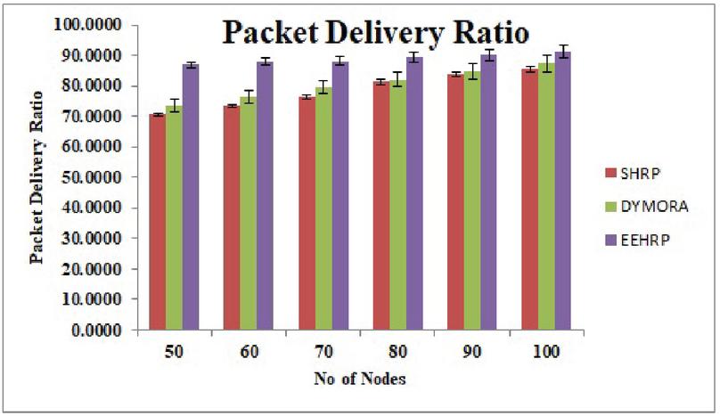
Figure 5 Packet delivery ratio.
6.2 Results Obtained
6.2.1 Packet Delivery Ratio (PDR)
The ratio of total number of packets received by the destination to the total packets generated by all the nodes is given by PDR. Figure 5 reveals EEHRP, SHRP, and DyMORA’s PDR. Due to MOO mechanism, EEHRP has PDR higher than DyMORA by a factor of 10.29% and by a factor of 13.28% than SHRP under various circumstances by reason that the packets are transmitted via optimum route. Due to MOO mechanism utilized by every node, the avg. energy consumption in the network is low, and this leads to increase in life of network. PDR endorses the proficient use of the sensor nodes for the transfer of the information packets.
6.2.2 Throughput
Throughput is a measure of how rapidly information can be send from end to end of a network. Figure 6.2 demonstrates EEHRP, SHRP, and DyMORA’s throughput. The reason that the throughput of EEHRP is higher than DyMORA as well as SHRP is, the hybrid nature of the protocol. Multiple metrics from different layers of WSN are optimized simultaneously for EEHRP development. With reference to SHRP as well as DyMORA, EEHRP has higher throughput of a factor of 39.19% and 22.71% respectively. The throughput validates the effectiveness of EEHRP for data forwarding.

Figure 6 Throughput.
6.2.3 Average Residual Energy (ARE)
ARE (Ref. Figure 7) is a ratio of sum of different node’s residual energies to the sum of total number of nodes. By reason of clustering as well as multi-hop communication amongst the sensor nodes within the cluster, EEHRP’s ARE is higher than DyMORA and smaller than SHRP. EEHRP outperforms DyMORA in terms of ARE by a factor of 7.7% and SHRP by 9.2 %. This energy saving prolongs the system’s life-expectancy in addition proves EEHRP’s usefulness.
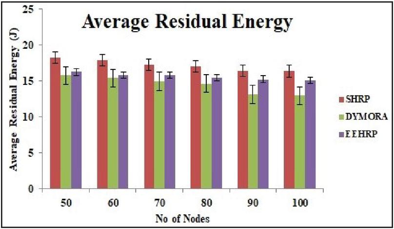
Figure 7 Average residual energy.
6.2.4 End-to-End Delay (Delay)
The delay is the time difference amid the first data packet generated by source node after an event is detected and the time when the data packet is received at the sink. EEHRP uses reaction time to find the best route as one of the optimization metrics, the delay is less than DyMORA by a factor of 38.18%. By a factor of 44.64%, SHRP is better in terms of delay compared with EEHRP. The reason is SHRP’s packet routing decisions are based on single metric instead of multiple metrics (Ref. Figure 8).
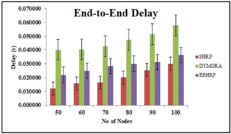
Figure 8 End-to-end delay.
6.2.5 Control Overhead (COH)
Equated with data packets, the number of control packets that are crucial for network communication is known as COH. Figure 9 illustrates the assessment of COH. EEHRP has COH lower than DyMORA and greater than SHRP. SHRP decides on the optimal route based on single metric. Additionally, in terms of COH equated with DyMORA EEHRP is effective. Compared with DyMORA, EEHRP decreases COH by a factor of 10.85%.
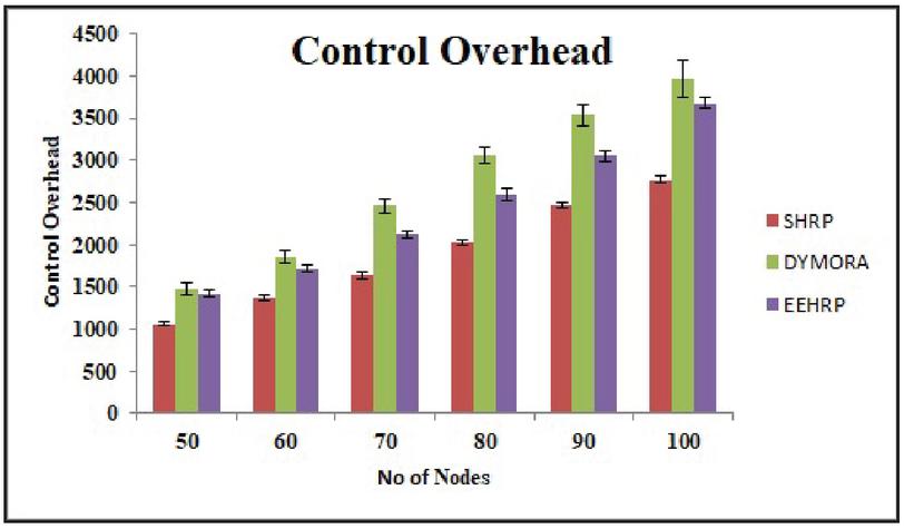
Figure 9 Control overhead.
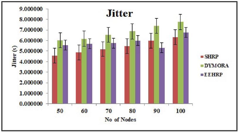
Figure 10 Jitter.
6.2.6 Jitter
In WSN, jitter means the delay variation in the packets’ arrival at the destination with any lost packets being ignored. Figure 10 illustrates the comparison of jitter. EEHRP has lower jitter than DyMORA and with reference to SHRP, EEHRP has comparable jitter. EEHRP improves jitter by a factor of 13.89% as compared to DyMORA. SHRP improves jitter by a factor of 8.16% as compared to EEHRP.
6.2.7 Normalized Routing Load (NRL)
NRL is calculated as an average of a total number of routing packets transmitted per data packet delivered to destination. As EEHRP incorporates MOO mechanism and it addresses QoS parameters from different layers in the WSN architecture. Routing overhead is less in EEHRP by 5.95% than DyMORA and higher by a factor of 10.17% than SHRP. Figure 11 gives a comparison of NRL between SHRP and DyMORA.
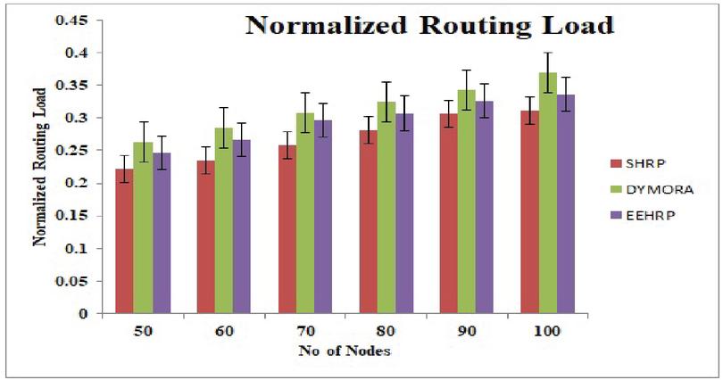
Figure 11 Normalized routing load.
7 Conclusion and Future Work
A novel QoS guaranteed energy-competent Multi-Objective Routing Protocol with cross-layer optimization mechanism called EEHRP for WSNs is put forward in this paper. EEHRP’s primary aim is to pick optimal route to the BS, subject to applying multi-objective concepts. EEHRP, SHRP, as well as DyMORA are simulated and their results are equated. In terms of PDR, Throughput, ARE, End-to-End Delay, COH, Jitter, as well as NRL, EEHRP is better protocol than DyMORA. EEHRP’s performance is equivalent to SHRP. It can be found in all the results obtained that the margin of error for the same no of sample data points is smaller in EEHRP than SHRP as well as DyMORA. Theoretically as well as practically EEHRP’s effectiveness is proved. By replacing homogeneous nodes with heterogeneous ones and by assigning mobility to them, the routing protocol can be further extended.
References
[1] J. Al-Karaki and A. Kamal, “Routing techniques in wireless sensor networks: a survey”, IEEE Journal, Wireless Communications, Vol. 11, Issue 6, pp. 6–28, 2004.
[2] N. Pantazis, S. Nikolidakis and D. Vergados, “Energy-Efficient Routing Protocols in Wireless Sensor Networks: A Survey”, IEEE Journal, Communications Survey and Tutorials, Vol. 15, Issue 2, pp. 551–591, 2013.
[3] N. Magaiaa, N. Hortab, R. Nevesb, P. Pereiraa and M. Correia, “A multi-objective routing algorithm for Wireless MultimediaSensor Networks”, ELSEVIER Journal, Applied Soft Computing, vol. 30 pp. 104–112, 2015.
[4] M. Bala Krishna and M. Doja, “Multi-Objective Meta-Heuristic Approach for Energy-Efficient Secure Data Aggregation in Wireless Sensor Networks”, Springer Journal , Wireless Personal Communication, Vol. 81, pp. 1:16, 2015.
[5] R. Bhardwaj, and D. Kumar, “MOFPL: Multi-objective fractional particle lion algorithm for the energy aware routing in the WSN”, Pervasive and Mobile Computing, Volume 58, 2019.
[6] Z. Sun, M. Wei, Z. Zhang, and G. Qu, “Secure Routing Protocol based on Multi-objective Ant-colony-optimization for wireless sensor networks”, Applied Soft Computing, Volume 77, 2019.
[7] K. Vijayalakshmi, and P. Anandan, “A multi objective Tabu particle swarm optimization for effective cluster head selection in WSN”, Cluster Computing, Vol. 22, pp. 12275–12282, 2019.
[8] A. Kaswan, V. Singh, and P. Jana, “A multi-objective and PSO based energy efficient path design for mobile sink in wireless sensor networks”, Pervasive and Mobile Computing, Volume 46, 2018.
[9] A. Raychaudhuri, and D. De, “Bio-inspired Algorithm for Multi-objective Optimization in Wireless Sensor Network”, In: De D., Mukherjee A., Kumar Das S., Dey N. (eds) Nature Inspired Computing for Wireless Sensor Networks, Springer Tracts in Nature-Inspired Computing. Springer, Singapore, pp. 279–301, 2020.
[10] V. K. Arora, V. Sharma, and M. Sachdeva, “ ACO optimized self-organized tree-based energy balance algorithm for wireless sensor network”, J Ambient Intell Human Computing, Vol. 10, pp. 4963–4975, 2019.
[11] M. M. Ahmed, E. H. Houssein , and A. E. Hassanien, et al., “Maximizing lifetime of large-scale wireless sensor networks using multi-objective whale optimization algorithm”, Telecommunication System, Vol. 72, pp. 243–259, 2019.
[12] H. Xiong, M. Peng, S. Gong and Z. Du, “A Novel Hybrid RSS and TOA Positioning Algorithm for Multi-Objective Cooperative Wireless Sensor Networks,” in IEEE Sensors Journal, Vol. 18, no. 22, pp. 9343–9351, 2018.
[13] N. Kulkarni, N. R. Prasad and R. Prasad, “G-MOHRA: Green Multi-Objective Hybrid Routing Algorithm for Wireless Sensor Networks”, International Conference on Advances in Computing, Communications and Informatics (ICACCI), New Delhi, India, pp. 2185–2190, 2014.
[14] N. Shabbir, and S. R. Hassan, “Routing Protocols for Wireless Sensor Networks (WSNs)”. Wireless Sensor Networks – Insights and Innovations, 2017.
[15] M. Shahzad, D. Nguyen, V. Zalyubovskiy, and H. Choo, “LNDIR: A lightweight non-increasing delivery-latency interval-based routing for duty-cycled sensor networks”, International Journal of Distributed Sensor Networks, Vol. 14(4), 2018.
[16] R. Kuntz, J. Montavont, and T. Noël, “Improving the medium access in highly mobile wireless sensor networks. Telecommunication Systems”. 2011.
[17] S. Özdemir, B. Attea and Ö. Khalil, “Multi-Objective Evolutionary Algorithm Based on Decomposition for Energy Efficient Coverage in Wireless Sensor Networks”, Springer Journal , Wireless Personal Communication, Vol. 71, pp. 195–215, 2013.
[18] X. Wei and L. Zhi, “The multi-objective routing optimization of WSNs based on an improved ant colony algorithm”, 6th International Conference on Wireless Communications Networking and Mobile Computing (WiCOM), pp. 1–4, 2010.
[19] S. Bhunia, S. Roy and N. Mukherjee, “Adaptive Learning assisted Routing in Wireless Sensor Network using Multi Criteria Decision Model”, International Conference on Advances in Computing, Communications and Informatics (ICACCI), New Delhi, India, pp. 2149–2154, 2014.
[20] D.Mahjoub and H.El-Rewini, “Adaptive Constraint-Based Multi-Objective Routing for Wireless Sensor Networks”, In Proceedings of IEEE International Conference on Pervasive Services, Istanbul, pp. 72–75, 2007.
[21] G. Valentini, C. Abbas, L. Villalba, and L. Astorga, “DyMORA :A Multi-Objective Routing Solution Applied on Wireless Sensor Networks”, IET Communications, Volume 4, Issue 14, pp. 1732–1741, 2010.
[22] R. Kumar, D. Kumar, “Multi-objective fractional artificial bee colony algorithm to energy aware routing protocol in wireless sensor network”, Springer, Wireless Networks, Vol. 22(5), pp. 1461–1474, 2015
[23] M. Garetto, E. Leonardi, “Analysis of Random Mobility Models with Partial Differential Equations”, IEEE Trans. Mobile Computing, vol. 6, no. 11, pp. 1204–1217, Nov. 2007.
Biographies

Nandkumar P. Kulkarni received Bachelor of Engineering (B.E.) degree in Electronics Engineering from Walchand College of Engineering, Sangli, Maharashtra, (India) in 1996. He has been with Electronica, Pune from 1996–2000. He worked on retrofits, CNC machines and was also responsible for PLC programming. In 2000, he received the Diploma in Advanced Computing (C-DAC) degree from MET’s IIT, Mumbai. In 2002, He became Microsoft Certified Solution Developer (MCSD). He worked as a software developer and system analyst in CITIL, Pune and INTREX India, Mumbai respectively. He has 23 years of experience both in industry and academia. From 2002 onwards he is working as a faculty in Savitribai Phule Pune University, Pune. Since 2007, he is working with SKNCOE, Pune as a faculty in IT Department. He completed his Master of Technology (M. Tech) degree with computer specialization from College of Engineering Pune (COEP) (India) in 2007. He has been awarded Ph.D. from Aarhus University, Denmark in 2019. His area of research is in WSN, VANET, and Cloud Computing. He has published 1 book chapter, papers in 18 International Journals, 15 papers in IEEE International conferences, and 03 papers in National Conferences. He is working on various committees at University and College.

Dnyaneshwar S. Mantri, PhD, IEEE Senior Member is graduated in Electronics Engineering from Walchand Institute of Technology, Solapur (MS) India in 1992 and received Masters from Shivaji University in 2006. He has awarded PhD. in Wireless Communication at Center for TeleInFrastruktur CTIF), Aalborg University, Denmark in March 2017. He has teaching experience of 25years. From 1993 to 2006 he was working as a lecturer in different institutes [MCE Nilanga, MGM Nanded, and STB College of Engg. Tuljapur (MS) India]. From 2006 he is associated with Sinhgad Institute of Technology, Lonavala, Pune and presently working as Professor in Department of Electronics and Telecommunication Engineering. He is member of IEEE, Life Member of ISTE and IETE. He has written three books, published 15 Journal papers in indexed and reputed Journals (Springer, Elsevier, and IEEE etc.) and 23 papers in IEEE conferences. He is reviewer of international journals (Wireless Personal Communication, Springer, Elsevier, IEEE Transaction, Communication society, MDPI etc.) and conferences organized by IEEE. He worked as TPC member for various IEEE conferences and also organized IEEE conference GCWCN2014 and GCWCN2018. He worked on various committees at University and College. His research interests are in Adhoc Networks, Wireless Sensor Networks, Wireless Communications, VANET, Embedded Security specific focus on energy and bandwidth.

Neeli Rashmi Prasad, Ph.D., IEEE Senior Member, Director of CTIF-USA, Princeton, USA, leading IoT Test-bed at Easy Life Lab and Secure Cognitive radio network test-bed at S-Cogito Lab and Professor at International Technological University (ITU), San Jose, CA, USA. She received her Ph.D. from University of Rome “Tor Vergata”, Rome, Italy, in the field of “adaptive security for wireless heterogeneous network” in 2004 and M.Sc (Ir.) degree in Electrical Engineering from Delft University of Technology, The Netherlands, in the field of “Indoor Wireless Communications using Slotted ISMA Protocols” in 1997. During her industrial and academic career for over 14 years, she has lead and coordinated several projects. At present, she is leading an industry-funded projects on Security and Monitoring (STRONG) and on reliable self-organizing networks REASON, Project Coordinator of European Commission (EC) CIP-PSP LIFE 2.0 for 65+ and social interaction and Integrated Project (IP) ASPIRE on RFID and Middleware and EC Network of Excellence CRUISE on Wireless Sensor Networks. She is co-caretaker of real world internet (RWI) at Future Internet. She has lead EC Cluster for Mesh and Sensor Networks and Counselor of IEEE Student Branch, Aalborg. She is Aalborg University project leader for EC funded IST IP e-SENSE on Wireless Sensor Networks and NI2S3 on Homeland and Airport security and ISISEMD on telehealth care. She is also part of the EC SMART Cities workgroup portfolio. She joined Libertel (now Vodafone NL), Maastricht, The Netherlands as a Radio Engineer in 1997. From November 1998 until May 2001, she worked as Systems Architect for Wireless LANs in Wireless Communications and Networking Division of Lucent Technologies, Nieuwegein, The Netherlands. From June 2001 to July 2003, she was with T-Mobile Netherlands, The Hague, The Netherlands as Senior Architect for Core Network Group. Subsequently, from July 2003 to April 2004, she was Senior Research Manager at PCOM:I3, Aalborg, 82 P. M. Pawar et al. Denmark. Her publications range from top journals, international conferences, and chapters in books. She has also co-edited and co-authored two books titled “WLAN Systems and Wireless IP for Next Generation Communications” and “Wireless LANs and Wireless IP Security, Mobility, QoS and Mobile Network Integration,” published by Artech House, 2001 and 2005. Her research interests lie in the area of Security, Privacy and Trust, Management or Wireless and wired networks and Energy-efficient Routing.

Ramjee Prasad is a Professor of Future Technologies for Business Ecosystem Innovation (FT4B1) in the Department of Business Development and Technology, Aarhus University, Denmark. He is the Founder President of the CTIF Global Capsule (CGC). He is also the Founder Chairman of the Global ICT Standardization Forum for India, established in 2009. GISFI has the purpose of increasing of the collaboration between European, Indian, Japanese, North-American and other worldwide standardization activities in the area of Information and Communication Technology (ICT) and related application areas. He has been honored by the University of Rome “Tor Vergata”, Italy as a Distinguished Professor of the Department of Clinical Sciences and Translational Medicine on March 15, 2016. He is Honorary Professor of University of Cape Town, South Africa, and University of KwaZulu-Natal, South Africa. He has received Ridderkorset of Dannebrogordenen (Knight of the Dannebrog) in 2010 from the Danish Queen for the internationalization of top-class telecommunication research and education. He has received several international awards such as: IEEE Communications Society Wireless Communications Technical Committee Recognition Award in 2003 for making contribution in the field of “Personal, Wireless and Mobile Systems and Networks”. Telenor’s Research Award in 2005 for impressive merits both academic and organizational within the field of wireless and personal communication, 2014 IEEE AESS Outstanding Organizational Leadership Award for: “Organizational Leadership in developing and globalizing the CTIF (Center for TeleInFrastruktur) Research Network”, and so on. He has been Project Coordinator of several EC projects namely, MAGNET, MAGNET Beyond, eWALL and so on. He has published more than 30 books, 1000 plus journal and conference publications, more than IS patents, over 100 Ph.D. Graduates and larger number of Masters (over 250). Several of his students are today worldwide telecommunication leaders themselves.
Journal of Mobile Multimedia, Vol. 17_1-3, 245–272.
doi: 10.13052/jmm1550-4646.171313
© 2020 River Publishers