Java Bytecode Control Flow Classification: Framework for Guiding Java Decompilation

Siwadol Sateanpattanakul, Duangpen Jetpipattanapong and Seksan Mathulaprangsan^*

Pattern REcognition and Computational InTElligent Laboratory (PRECITE Lab), Department of Computer Engineering, Faculty of Engineering at Kamphaengsean, Kasetsart University, Nakhon Pathom, Thailand

E-mail: sidol.sat@gmail.com; duangpenj@gmail.com; seksan.m@ku.th

*Corresponding Author

Received 24 September 2020; Accepted 31 July 2021; Publication 29 October 2021

Abstract

Decompilation is the main process of software development, which is very important when a program tries to retrieve lost source codes. Although decompiling Java bytecode is easier than bytecode, many Java decompilers cannot recover originally lost sources, especially the selection statement, i.e., if statement. This deficiency affects directly decompilation performance. In this paper, we propose the methodology for guiding Java decompiler to deal with the aforementioned problem. In the framework, Java bytecode is transformed into two kinds of features called frame feature and latent semantic feature. The former is extracted directly from the bytecode. The latter is achieved by two-step transforming the Java bytecode to bigram and then term frequency-inverse document frequency (TFIDF). After that, both of them are fed to the genetic algorithm to reduce their dimensions. The proposed feature is achieved by converting the selected TFIDF to a latent semantic feature and concatenating it with the selected frame feature. Finally, KNN is used to classify the proposed feature. The experimental results show that the decompilation accuracy is 93.68 percent, which is obviously better than Java Decompiler.

Keywords: Decompilation, feature selection, latent semantic indexing, genetic algorithm.

1 Introduction

Software maintenance, which is a process of cognition, knowledge acquisition, and comprehension for the system, can be considered to be the most important part of software engineering nowadays since it consumes around 70 percent of the programming process [1]. Without source code, decompilation is the main process for software maintenance. This process is a reverse transformation from a low-level language to a high-level language [2]. In legitimate use, decompilation is used to recover the lost source codes for crucial applications [3].

Java bytecode is a form of low-level data that represents source code behavior in an executable form. Although it retains some types of information, e.g., fields method returns and parameters, but does not contain some other important information, e.g., local variables. Generally, the local variable type is one of the required information to analyze. The others include flattening of stack-based instructions and structuring of loops and conditionals.

If a simple understanding of a program is the purpose of decompilation, the syntactical correctness of a completely decompiled program might not be the main goal. Moreover, in case of a company lost their application’s source code and want to continue development, the recovery of correct source code is needed. They must decompile and attempt to recover the originally lost source, which is easy to maintain and directly suitable for use by the clients in their rewriting application. This is a crucial characteristic of decompiler, which has to do decompilation [3].

In the decompiler research, J. Hamilton et al. [4] evaluated Java decompiler including the existing commercial, free and open-source, which include 9 decompilers. Their experiment focused on 6 categories of usual Java compiler including Fibonacci, Casting, InnerClass, TypeInference, TryFinally, and ControlFlow. The effectiveness of those decompilers was reported that Dava, Java Decompiler, and JODE are the best decompiler. And each decompiler has different advantages, which can do perfect decompilation in many categories. However, there is no perfect decompilation in the ControlFlow category, which represents the ambiguity of those statements. Jozef et al. [5] repeated the experiment and confirmed a similar result. Moreover, Nicolas et al. [6, 7] that there are at least three points including if statement that decompiled source codes are different from the original code.

The category of decompilation can be divided into two groups, which are non-machine learning and machine learning. For the first group, Nicolas et al. [7] evaluated eight non-machine learning Java decompilers. Each of them has different advantages in syntactic correctness and semantically equivalence. And they used them to build Arlecchino, their proposed meta-decompiler. For the second group, Miller et al. [8] proposed a novel dissemble technique to deal with the loss of information during the compilation process. This technique computes a probability to indicate the instruction. While Schulte et al. [9] prepared “big code” database. They used evolutionary search to find the equivalent binary and gain its equal source code. Katz et al. [10] used recurrent neural network (RNN) for decompiling binary code, which generated more similar human-written code.

To improve the performance of decompilation in the ControlFlow category, this paper introduces a methodology that guides the decompiler to select appropriate characteristics of the control flow statement during the decompilation process. In our framework, we apply bigram to trans form bytecode to TFIDF. Then a genetic algorithm (GA) is incorporated for selecting important features that are processed using latent semantic indexing (LSI). Finally, the selected features are classified using K-nearest neighbor (KNN).

In Section 2, we describe preliminary knowledge. Then, the proposed framework is introduced in Section 3. Section 4 provides the experimental results and the discussion is presented in Section 5. Finally, the conclusion and future work are considered in Section 6.

2 Preliminaries

2.1 Java Bytecode Structure

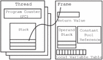
In this section, we provide the basics of Java bytecode structure. In brief, it is Java Virtual Machine (JVM) processes regarding the execution of the bytecode. A JVM is a stack-based machine that contains heaps and many threads in the runtime data area [11]. Each thread has a JVM stack that stores frames. The frame consists of an operand stack, an array of local variables, and the execution environment which references the runtime of a constant pool of the current method class (Figure 1).

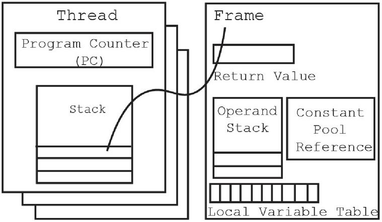
Figure 1 Java bytecode structure.

The local variable table or the array of local variables contains several of the variables that are used by JVM during the execution of the method. Any one of the local variables refers to all method parameters and other locally defined variables. The local variable table is used to hold the values of the local variables with sequential formatting. For example, the frame is a constructor or an instance of the method stored at index 0. Then, the next instruction contains index 1, and so on. The size of the local variable table is defined at compilation time by using formal method parameters and the number of local variables. The final structure of the bytecode concept is the operand stack having 32-bit slots. The operand stack is used to push and pop the values of virtual machine instructions.

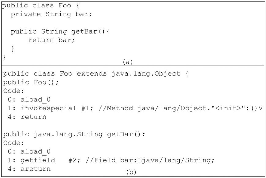
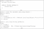
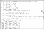
Figure 2 Examples of Java codes: (a) Java source code and (b) Java bytecode.

For working on JVM processes, the bytecode contains many kinds of instructions. Each instruction consists of a one-byte opcode followed by zero or more operands. These opcodes are put into the operand stack when executing the method. For example, a POJO contains an field and getter method (Figure 2(a)). The getBar() method’s bytecode consists of three opcode instructions (Figure 2(b)). The opcode has individual characteristics depending on the objective. For example, i_load_0 is an opcode that has a ‘i’ as a prefix. The prefix ‘i’ is used to manipulate an integer value. In the same way, other opcodes must have a prefix corresponding with the data type. For this example, Figure 3(a), the aload_0 is the first opcode which stores at index 0 in the local variable table. The next opcode is getfield. This opcode is used to fetch data from the field that corresponds with its object at execution time. Then, the instruction ‘this’ is popped from the top of the operation stack. At the same time, #2 is used to create an index at the constant pool which refers to a variable bar.

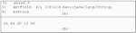
For this step, the variable bar is loaded onto the operation stack and is ready to perform. The last opcode is the areturn that refers to the return type of the method. The areturn instruction is loaded by JVM to the top of the operand stack, which is also popped and pushed onto the operand stack during execution time. The getBar() has 3 index values (0, 1, and 4) that correspond to the byte array for the method. The byte array corresponds to the index, which stores the opcode from its parameter. Because the method getBar() has no parameter, it occupies one byte in the bytecode array for storing the opcode aload_0 (0x2A) at index 0. The next instruction is getfield (0xB4), which is stored at index 1 and the local variable table uses two bytes to store this instruction. Hence, index 4 contains the areturn (0xB0) instruction. The local variable table is constructed inside the constant pool. Figure 3(a) presents the bytecode instruction in the getBar() method. The Java class file contains the bytecode that can be viewed using the hexadecimal editor. Figure 3(b) presents the hexadecimal format of this method.

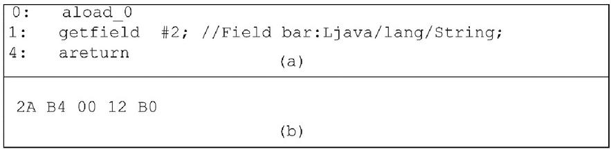
Figure 3 Java bytecode and hexadecimal format: (a) Java bytecode instruction. (b) Java bytecode in hexadecimal format.

As mentioned above, there is a single statement in getBar() method. The bytecode structure uses three opcodes to describe its function. The programming environment contains many statements and expressions; hence there are many opcodes in a real-world application. For this reason, the bytecode structure must be investigated expertly and carefully.

2.2 Term Frequency-Inverse Document Frequency

TFIDF is a weighting strategy, which is used to indicate the importance of words or terms in an observed document. The TFIDF scheme assigns weighting terms as a product of the term frequency (TF) and inverse document frequency (IDF) of an observed document. The TF of the term $t$ can be computed by normalizing the term’s appearance frequency in an observed document $d$ as follows.

TF (t, d) = \frac{Term t frequency in document d}{Total word in document d} .

(1)

IDF indicates the importance of the term $t$ among the various documents in the whole dataset, which is calculated as follows.

IDF (t) = l o g_{e} \frac{Total document s}{documents with term t} .

(2)

The TFIDF of the term $t$ in an observed document $d$ can be computed as follows.

TFIDF (t, d) = TF (t, d) \times IDF (t) .

(3)

The TFIDF value of the term $t$ in document $d$ describes its importance to the whole dataset. On the one hand, a high score means the term $t$ appears in a small number of documents and is more meaningful, whereas a low score indicates that the term $t$ generally occurs in many documents and is less meaningful.

With the TFIDF technique, each document can be transformed into a vector, in which each element contains the TFIDF score of the corresponding term. Such a TFIDF vector contains non-negative values, though some elements might be zero where those terms do not occur in the observed document. TFIDF vectors can be used to construct the term-document matrix, in which each row represents the TFIDF vector and each column is its corresponding term.

2.3 Latent Semantic Index

The LSI is an information retrieval technique that uses a vector space model to describe the hidden information in the original data [12]. The vector space model represents the relationship between a set of documents and the terms by using a one-hot encoding technique. This technique involves count vectorization because it counts the occurrence of a word. The LSI is used to construct word embedding that rearranges the document as a term-document matrix. The LSI takes advantage of the reduced dimension [12, 13]. It improves vectors by replacing approximation value from single value decomposition (SVD) [14–16]. SVD is similar to principal component analysis (PCA), which is used to reduce noise data while preserves the original signal [17]. By using LSI, the transformed vector has improved data that is a better representation for text processing [18–20].

Let $A$ be an $m$ -by- $n$ dimension matrix. We can perform SVD to decompose matrix $A$ into the product of three matrices as follows.

A = U Σ V^{T} .

(4)

The columns of $U$ and $V$ are orthonormal while $Σ$ is a diagonal matrix. These matrices have greater robustness regarding numerical error than the regular form. We can reduce the dimensions of the factors by selecting rank $k$ and computing the approximated matrix $A_{k}$ as follows:

A_{k} = U_{k} Σ_{k} V_{k}^{T},

(5)

where $U_{k} \in R^{m \times k}$ is the first $k$ columns of $U$ . $V_{k}^{T} \in R^{k \times n}$ is the first $k$ rows of $V^{T}$ . The diagonal matrix $Σ_{k} \in R^{k \times k}$ is the first $k$ rows and $k$ columns of $Σ$ . Each column of $V_{k}^{T}$ represents the transformed coordinates of the corresponding column of $A$ in $k$ -dimensional space. Any vector $q$ with $m$ elements can be transformed to such $k$ -dimensional space as follows:

q^{'} = q^{T} U_{k} Σ_{k}^{- 1} .

(6)

The coordinates in $k$ -dimensional space can be used in many distance measurement methods such as the cosine distance (COS), the Euclidean distance (EUC), and the Manhattan distance (MAN).

3 The Proposed Method

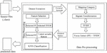
The main idea of this study is to use bytecode analysis and classification to enhance Java decompilation. To achieve this, we use a bytecode token-based approach on bigram that cooperates with TFIDF, GA, LSI, and KNN. In this section, we describe all the related steps of the proposed system, which has three modules: dataset extraction, data pre-processing, and data processing (Figure 4).

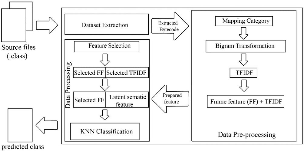
Figure 4 System overview of our framework.

3.1 Dataset Extraction

To evaluate the proposed approach, the dataset was created from two kinds of sources, namely the bytecode instruction and the stack frame. Firstly, the bytecode instruction is divided into a piece of code, which is a block of statements (also known as a document). Each block of statements is composed of many kinds of statements. To make the dataset concise, our extraction strategy focuses only on if, ifElse, ifElseIf, and nested if statement from the document and transforms them to a sequence the bytecode. For example, Figure 5(a) presents a document composed of an if statement and a block of statement. We remove other statements except for the if statement, which is shown in Figure 5(b).

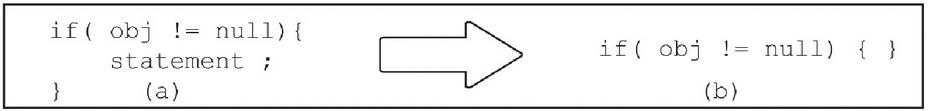
Figure 5 Data collection process: (a) if statement with block of statement.(b) if statement that removes other statements.

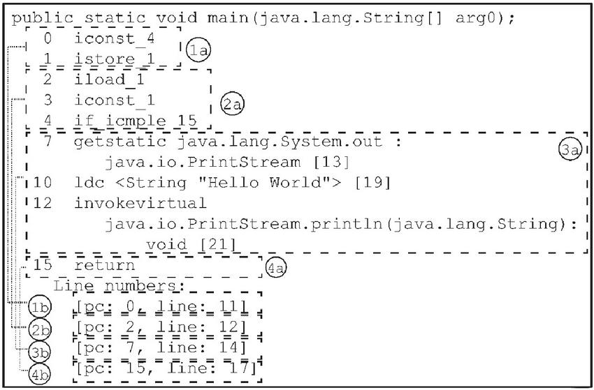
Figure 6 Instruction frame: (1a) number of instructions; (1b) scope of each frame.

In this step, we extract the list of the bytecode instruction $S = [s_{1}, \dots, s_{n}]$ , which is directly converted from the remaining sequence of statements from the .class file. Note that $s_{i}$ is the $i$ th bytecode instruction and $n$ is the number of bytecode instructions in the statement sequence. The second extraction source is from the stack frame. Normally, the bytecode structure has a Java stack composed of several stack frames. Such stack frames store the indices of the instruction set, which describes Java method invocation. We collect the list of the number of jump instructions in each frame. Note that $T = [t_{1}, \dots, t_{m}]$ is the list of the number of jump instructions, $t_{i}$ is the number of jump instructions in frame $i$ th, and $m$ is the number of frames in the Java method. Figure 6 presents the strategy of our data collection.

Table 1 Groups of instruction

Group	Type of Instruction	Opcodes
1	Constants	00–20
2	Loads	22–53
3	Stores	54–86
4	Stack	87–95
5	Math_1	96–131
6	Math_2	132
7	Conversion	133–147
8	Comparison_1	148–152
9	Comparison_2	153–166 , 198–199
10	Control_1	167–169
11	Control_2	170–171
12	Control_3	172–177
13	References_1	178–186
14	References_2	187–190
15	References_3	191–195
16	Others	196–197 , 200–201

3.2 Data Pre-processing

The main pre-processing step in this study is the construction of features from two sets of data ( $S$ and $T$ ). To produce compact sets of features that represent the dependency relationship among the documents, the bytecode instruction $s_{i}$ is transformed to its corresponding category. Table 1 presents a list of defined categories of bytecode sequence $Y = [y_{1}, y_{2}, \dots, y_{m}]$ where $y_{i}$ represents the $i$ th category of instruction $s_{i}$ , and $n$ is the number of bytecode instructions in the statement sequence.

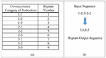
The data type used in this study is the sequence of bytecode categories, in which each word has some relationship with its neighbors. To take advantage of such information, we use bigram analysis for all instruction categories. The bigram of instruction categories represents co-occurrence between connected categories of instructions y $_{i}$ and y $_{i + 1}$ . For example, for the category of bytecode sequence $Y = [1, 2, 3, 2, 2]$ , to change an input string, this process constructs the mapping table that defines the conversion between adjacent categories of bytecode and bigram number as shown in Figure 7(a). After mapping the table, this process replaces the adjacency category of bytecode $y_{i}$ and $y_{i + 1}$ by its corresponding bigram number into a new co-occurrence structure as [2, 6, 8, 5]. Figure 7(b) illustrates how to apply bigram to build a new string for the input sequence. Let $B^{i} = [b_{1}^{i}, \dots, b_{N}^{i}]$ be a bigram sequence of the document $i$ , where $N = n - 1$ .

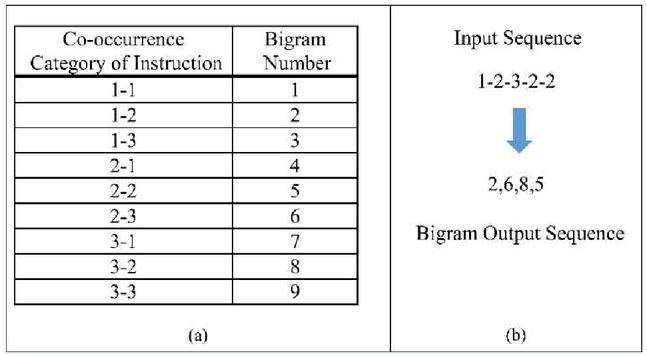
Figure 7 Bigram transformation process: (a) representing an example of the mapping table. (b) representing the bigram transformation process.

We denote $h$ as the number of documents. After that, we construct a term-by-document matrix $D^{TD}$ from $B^{i}$ . Note that $D^{T D}$ is an h-by-l matrix where $l$ is the number of bigram instruction categories. The element $d_{i j}$ contains the number of bigrams times the number at $i$ th co-occurrence in document $j$ th. Then $D^{T D}$ is transformed to $D^{T F I D F}$ by using Equation (3). Matrix $τ$ can be computed to represent the number of jump instructions in each frame of all documents. Denote $M$ as the maximum number of frames in our collected document. $τ_{i j}$ is the number of jump instructions within the $j$ th frame of the $i$ th document.

Finally, we concatenate features from matrices $D^{TFIDF}$ and $τ$ to create the training dataset $P \in R^{h \times u}$ as $P = [τ D^{TFIDF}]$ . Note that row $i$ of $P$ is the feature vector of document $i$ which composed of $i$ th row of $D^{TFIDF}$ , the list of the numbers of jump instructions of document $i$ , and $u$ is $l + M$ .

3.3 Data Processing

3.3.1 Features selection

GA is applied in this study for features selection (FS), which aims to remove redundancies and to select relevant features. In GA, the quality of the population has a direct effect on the success rate, which is a key performance factor. Achieving good performance depends on quantity and diversity. The population size must start with a proper number. The mating contains a pool of these chromosomes. Each generation of GA is a chromosome that has an optimal fitness value [21–23]. In this step, the input data $P$ must be selected by the chromosome $c^{FS}$ . It is encoded as an $u$ elementary binary vector, where $c^{F S} = {[c_{1}^{FS} c_{2}^{F S} \dots c_{u}^{FS}]}^{T}$ . Each element $c_{i}^{F S} \in {0, 1}$ represents the selection or elimination features of $P$ in column $i$ . We denote the selected features of $τ$ and $D^{TFIDF}$ as $τ^{FS}$ and $D^{FS}$ respectively.

3.3.2 LSI and KNN classification

KNN is a lazy-learning algorithm that captures information on all training cases. It takes the $k$ closest neighbors to a point (closest depends on the distance metric chosen) and each neighbor constitutes a vote for its label. Simply, the KNN algorithm is a classification algorithm based on feature similarity.

To classify by KNN, we transform the $D^{FS}$ to LSI called $D^{LSI}$ . Finally, we construct the input for the classification algorithm as $P^{FS} = [τ^{FS} D^{LSI}]$ . The accuracy of our classification algorithm becomes the fitness value for to evaluation of the next chromosome $c^{FS}$ .

After the document (training data and validation data) has been transformed by the LSI into new query vector coordinates, it has an appropriate format ready has to be used for measurement, with the EUC being the most common matrix used, while the MAN is also a very useful matrix for continuous variables. Therefore, our approach selects the EUC and MAN for the measurement distance matrix. The EUC can be defined as:

d_{EUC} (p, q) = \sqrt{\sum_{i = 1}^{n} {(p_{i} - q_{i})}^{2}} .

(7)

The MAN can be defined as

d_{MAN} (p, q) = \sum_{i = 1}^{n} | p_{i} - q_{i} | .

(8)

Note that $p = {[\begin{matrix} p_{1} & p_{2} & \dots & p_{n} \end{matrix}]}^{T}$ and $q = {[\begin{matrix} q_{1} & q_{2} & \dots & q_{n} \end{matrix}]}^{T}$ .

4 Experimental Results

To reveal the performance of Java Bytecode Control Flow Classification framework, a set of experiments and their results are presented in this section. Each experiment aims to show the significant factor that can improve the system performance. Firstly, the frame feature on the framework is explored. Then, the classification performance with bigram is exhibited. After that, the proper number of nearest neighbors and SVD ranks, which effect on classification performance, is evaluated. Finally, the comparison of classification performance between the proposed framework and Java Decompiler is presented.

Table 2 Number of test cases for each class in the three datasets

	Class

Dataset	1	2	3	4	5	Total
Eclipse.jdt.core	45	441	225	66	148	925
Apache BCEL 6.3.1	2	8	50	11	11	82
Apache Ant 1.9.14	31	322	267	67	46	733
Total	78	771	542	144	205	1740
%	4.48	44.31	31.15	8.28	11.78

We used three Java open source projects, named Eclipse.jdt.core 4.5.0 [24], Apache Commons BCEL 6.3.1 [25], and Apache Ant 1.9.14 [26] for training and testing our algorithm. The details of the datasets are described in Table 2. After data extraction, we had 1740 records, which explain the number of classes from each open source in Table 2. To clarify the category of if statement, we defined five classes of if statement as shown in Table 3. All experiments were conducted by using Python 3.5.2 with dependency libraries such as Numpy 1.16.1 and Scikit-learn 0.19.1 on a computer with an Intel(R) Core $^{(TM)}$ i3-2120 CPU @ 3.30 GHz and 8 GB RAM, running Ubuntu 16.04.5 LTS.

Table 3 Categories of if statement

Class	Statement
1	if(expr && expr && expr) stmt
2	if(expr && expr) stmt
3	if(expr) stmt else stmt
4	if(expr) stmt else if(expr) stmt else stmt
5	if(expr) if(expr) stmt

4.1 Frame Feature Evaluation

As we mentioned above, this section investigates the effectiveness of the frame feature. We conducted 5-fold cross validation to evaluate the performance of our methodology. The mean accuracy as well as its standard deviation were reported. Firstly, we evaluated the dataset using three distance measurement methods (COS, EUC, and MAN).

In the first experiment, we transformed the sequence of bytecode to TFIDF terms. Then, the frame feature was applied to TFIDF and compared both datasets with three measurement methods. The results in Table 4 present that the classification performance increases by applying frame feature, from 65.46 to 87.99 for COS, 71.72 to 89.66 for EUC, 72.59 to 88.56 for MAN. Furthermore, the standard deviation of all measurements also decreases, from 7.45 to 1.08 for COS, 2.30 to 1.80 for EUC, and 2.42 to 1.53 for MAN. These results reveal the advantage of the frame feature, which improves the accuracy and stability of classification.

Table 4 The accuracies of TFIDF and TFIDF with frame feature on three measurement methods

Methods	No Frame Feature	Frame Feature
COS	65.46(7.45)	87.99(1.08)
EUC	71.72(2.30)	89.66(1.83)
MAN	72.59(2.42)	88.56(1.53)

4.2 Performance Evaluation of Bigram and Number of Nearest Neighbor

In the second experiment, we compare two kinds of the dataset. The first dataset is the category of bytecode sequence, which is transformed to TFIDF and concatenated with frame feature (No_Bigram). For the second dataset, we created it as same as the first dataset, except applying bigram at the beginning step. After that, we evaluated both EUC and MAN distances. Note that the COS similarity was ignored here because it has less efficiency than other distance measurements.

The result in Table 5 shows the effectiveness of the bigram technique. the mean accuracy is improved from 89.08 to 91.55 percent and from 89.08 to 91.55 percent for EUC and MAN respectively. When applying bigram, the bytecode form is a sequence that properly extracts relationship information between bits. For this reason, the accuracy of the Bigram framework is higher than the No_Bigram framework for both measurement methods.

Table 5 The accuracy of No_Bigram and Bigram on EUC and MAN distance methods

Methods	No_Bigram	Bigram
EUC	89.08(1.20)	91.55(1.01)
MAN	89.37(1.95)	91.03(1.29)

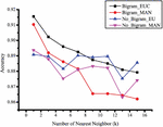
The accuracy of KNN depends on the number of the assigned k-nearest neighbors. This experiment investigated the appropriate number of $k$ neighbors. Figure 8 demonstrates the mean accuracies of the KNN algorithm based on two distance measurements. The highest score was achieved when $k$ was set to 1 for both measurement methods.

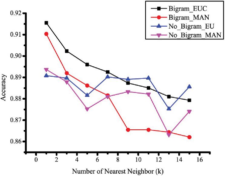
Figure 8 Accuracy of each method with differing numbers of nearest neighbors.

Table 6 The accuracy of NB_SVD and B_SVD on EUC and MAN distance methods

Methods	NB_SVD	B_SVD
EUC	91.32 (1.17), r $=$ 2	92.18 (1.97), r $=$ 12
MAN	91.26 (1.53), r $=$ 2	91.84 (1.91), r $=$ 13

4.3 Low-rank Approximation

In this experiment, we applied SVD on TFIDF to No_Bigram and Bigram datasets and denoted them with NB_SVD and B_SVD, respectively. SVD projects an n-dimensional space onto an r-dimensional space, where $n > r$ and $n$ is the number of word types in the collection [16]. Each $r$ value contributes the classification accuracy of each rank, and each value has an individual accuracy. This experiment investigated the SVD rank representing the highest accuracy based on a low-rank approximation technique [27]. Table 6 presents the optimal SVD rank from all measurement methods based on the LSI methodology. The highest accuracy is 92.18 on SVD rank 12 from B_SVD, which is performed by EUC measurement method.

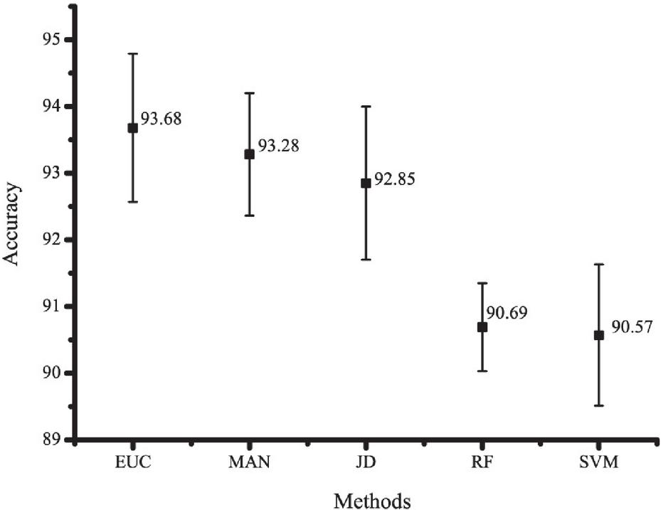
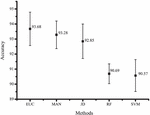
Figure 9 Accuracy of our framework using MAN and EUC measurement distance methods compared with Java decompiler, random forest, and support vector machine.

4.4 Performance of GA on TFIDF and Latent Dimension Space

We investigated GA to reduce the dimensional space. GA is a sub-optimal search method [18, 28], which is used to provide the approximated value for the optimal solution. To find the potential of the method, we applied GA to No_Bigram and Bigram datasets and transformed them to SVD. Then, they were evaluated by using two measurement methods, EUC and MAN (see Section 3.3.2) compared with the original JD. To position the proposed frameworks clearly, we also compared them with two well-known classifiers, which are random forest (RF) and support vector machine (SVM). Support vector machine is one of the most successful classifiers in many applications including text classification. Hence, many researchers used SVM with dimensionality reduction to improve their studies [29–31]. Random forest is also a famous classification method for text classification [32]. It provides a good computational cost with high accuracy in both document categorization [33] and text classification [34]. As shown in Figure 9, the highest accuracy is own by EUC, which is 93.68 percent. While MAN and JD achieve 93.28 and 92.85 percent, respectively.

4.5 Performance of the Java Decompiler

To evaluate the performance of the other Java decompiler, we selected an effective Java Decompiler (JD) tool named JD to use as a baseline to compare with our proposed framework. JD is an efficient decompiler, which received the highest score when compared with other Java decompilers and it has been accepted as one of the best tools for decompiling Java bytecode [4], which is used by current studies.

Table 7 Confusion matrix for JD tool

	Predicted Class

		1	2	3	4	5
Actual class	1	96.15	3.85	0.00	0.00	0.00
	2	0.00	99.61	0.00	0.26	0.13
	3	0.37	0.18	99.26	0.18	0.00
	4	2.08	2.08	0.69	95.14	0.00
	5	14.63	37.56	0.00	0.00	47.80

Table 8 Confusion matrix for our framework

	Predicted Class

		1	2	3	4	5
Actual class	1	85.90	0.00	2.56	1.28	10.26
	2	0.00	95.85	0.13	0.13	3.89
	3	0.00	0.74	96.49	1.66	1.11
	4	0.69	2.08	5.56	89.58	2.08
	5	6.34	4.39	3.90	1.46	83.90

In term of mean accuracy, the proposed framework achieves 93.68 percent, which is 0.83 percent higher than those of JD. For a more detailed comparison, the performances of both were compared by using a confusion matrix as shown in Tables 7 and 8. Table 2 presents that there are five classes of statement and the test cases of class 1 to 5 is 4.48, 44.31, 31.15, 8.28, and 11.78 percent, respectively. As shown in Table 8, the accuracy of the proposed framework for class 5 is 83.90 percent, which is hugely better than JD (47.80 percent). For classes 2 and 3, the accuracies of our framework are 95.85 and 96.49 percent, while the accuracies of JD are 99.61 and 99.26 percent, respectively. For classes 1 and 4, the accuracies of our framework are 85.90 and 89.58 percent, while the accuracies of JD are 96.15 and 95.14 percent, respectively.

Table 9 Confusion matrix for JD with an extension module

	Predicted Class

		1	2	3	4	5
Actual class	1	96.15	0.00	0.00	0.00	3.85
	2	0.00	95.85	0.00	0.26	3.89
	3	0.37	0.18	99.26	0.18	0.00
	4	2.08	2.08	0.69	95.14	0.00
	5	14.63	1.95	0.00	0.00	83.41

Moreover, the proposed framework can be used as an extension module to assist the other decompilers, such as JD, in classifying their ambiguous input. Table 9 illustrates the confusion matrix of the classification accuracies for JD by using our framework as an extension module. This module is used by JD to predict the aforementioned inputs when JD has predicted as class 2. The classification performance is increased from 47.80 to 83.41 in class 5. The decompilation accuracy has a 2.6% improvement, from 92.85 to 95.40%, when includes an extension module.

5 Discussion

The first experiment focused on evaluating the performance of the input data with and without frame feature on three distance measurement methods (COS, EUC, and MAN). Its results are shown in Table 4. Without frame feature, the classification accuracy of COS, EUC, and MAN is 65.46, 71.72, and 72.59 respectively. With frame feature, the classification accuracies increase to be 87.99, 88.56, and 89.66 respectively. These results reveal the effectiveness of the frame feature, which improves the classification accuracy significantly. Moreover, the standard deviations of all measurements are narrow, which means the stability of the classification system. Then, the input data were transformed into the TFIDF matrix after which we applied the bigram technique to the TFIDF matrix and measured the distance of two compared features in the classification step based on two significant methods (EUC and MAN). The effect of using bigram and the various distance measurements are evaluated in this section. Table 5 illustrates the classification accuracy in those various processing strategies. Without bigram, the classification accuracy of the two distance methods was 89.08 and 89.37 percent. With bigram, the classification accuracy of the two distance methods was 91.55 and 91.03. These experimental results reveal two notable points. First, the frame feature and instruction feature have a major impact on the classification of the dataset. Second, performance is improved when applying the bigram technique. This means that there is a relationship between each pair of bytecode instructions. Therefore, bigram is the relevant technique to take advantage of this information in bytecode classification.

Because all measurement methods were performed on the KNN classifier, the number of nearest neighbors directly affects the classification accuracy and this was also investigated. Figure 8 illustrates the accuracy of the KNN classification with various numbers of neighbors. The $k = 1$ shows the highest accuracy of all measurements and datasets. The reason for this phenomenon is that the bytecode of each class consists of various programming patterns from many conditions and data types. This makes the bytecode format of each class be formed in multiple variations. As a result, the data from the same class are distributed in different locations in the feature space. Conversely, for the same reason, many classes have similar bytecodes in some cases. This makes some data from different classes to be intersected in the feature space. Therefore, the use of $k = 1$ can be better aided in classification than $k > 1$ , which might lead to the intersection problem of the different classes as we mentioned above. The result of this experiment represents the nature of text data, which is quite similar. For this reason, we use this $k$ neighbors on the rest of the experiments. Table 6 shows the classification accuracies when we applied bigram and decomposed the TFIDF feature by SVD to produce the latent space dimensions. The number of TFIDF features was reduced by the low-rank approximation method. Without a severe loss of descriptiveness, we found different optimum accuracies when we reduced the latent dimension based on the two measurement methods (EUC and MAN). The highest accuracies for each combination were: B_SVD, 92.18 percent on SVD rank 12; and B_SVD, 91.84 percent on SVD rank 13.

To improve the performance of the system, some features have to be removed before decomposing by SVD. Because GA can be used to clean up inappropriate features, it has the potential to solve the very large number of factors in this dataset. Therefore, we applied GA to select the proper features on TFIDF with decomposition by SVD. The results in Figure 9 show that after applying this strategy, the recognition rates increase to 93.68 and 93.28 for EUC and MAN respectively. These are higher than JD tool, which its recognition rate is 92.85.

Tables 7 and 8 present the classification performance of JD tool and our framework in terms of the confusion matrix. Compared with JD, the overall performance of the proposed framework is noticeably better than JD, especially when performed on class 5. The proposed approach and JD have quite similar performances when performed in classes 2 and 3. Meanwhile, our approach has lower accuracies than JD for classifying classes 1 and 4. However, these data are seldom found in real-world applications. Note that, the bytecode from classes 3 and 4 has an obvious sequence, which can be easily detected by JD. On the other hand, the bytecode from class 2 and 5 has a quite similar sequence, which made a lot of fault classification to the classifier, from class 5 to class 2 (see Table 7). In this situation, our method has more accurate than JD to classify it. Overall, our approach has a potential that can be used as an extension module to support the others decompiler tools such as JD and Arlecchino for decompiling bytecode.

6 Conclusion and Future Works

This paper focuses on the framework to correct recovering control flow statement of Java source from the Java bytecode as a classification problem. In the framework, firstly, Java bytecode is transformed into a frame feature concatenated with the latent semantic feature. The frame feature is extracted directly from the bytecode. While the latent semantic feature is extracted by transforming the Java bytecode to bigram and then TFIDF. Secondly, both of them are fed to the genetic algorithm to reduce their dimensions. Thirdly, the proposed feature is achieved by converting the selected TFIDF to a latent semantic feature and concatenating it with the selected frame feature. Finally, each composed feature is classified by KNN. The classification accuracy of our approach is 93.68 percent based on specific statements, which can be used as a guideline for decompiling and recovering the correct original form of the source code. The next step of research can be expanding the framework to other complex condition statements and other control statements. Moreover, other word-embedding models such as Word2vec, GloVe, and TextRank as they are particularly computational and efficiently predictive model for learning word embeddings from raw text, as well as other efficient classification models such as a number of deep learning approaches, are included in our area of interest.

References

[1] I. Sommerville, Software Engineering, 9th ed. Boston, MA, USA: Addison Wesley, 2011.

[2] G. Nolan, Decompiling Java, 1st ed. Berkeley,CA: Apress, 2004.

[3] M. V Emmerik and T. Waddington, “Using a decompiler for real-world source recovery,” in 11th Working Conference on Reverse Engineering, 2004, pp. 27–36.

[4] J. Hamilton and S. Danicic, “An Evaluation of Current Java Bytecode Decompilers,” in 2009 Ninth IEEE International Working Conference on Source Code Analysis and Manipulation, 2009, pp. 129–136.

[5] J. Kostelanský and L’. Dedera, “An evaluation of output from current Java bytecode decompilers: Is it Android which is responsible for such quality boost?,” in 2017 Communication and Information Technologies (KIT), 2017, pp. 1–6.

[6] N. Harrand, C. Soto-Valero, M. Monperrus, and B. Baudry, “The Strengths and Behavioral Quirks of Java Bytecode Decompilers,” in 2019 19th International Working Conference on Source Code Analysis and Manipulation (SCAM), 2019, pp. 92–102.

[7] N. Harrand, C. Soto-Valero, M. Monperrus, and B. Baudry, “Java decompiler diversity and its application to meta-decompilation,” J. Syst. Softw., vol. 168, p. 110645, 2020.

[8] K. Miller, Y. Kwon, Y. Sun, Z. Zhang, X. Zhang, and Z. Lin, “Probabilistic Disassembly,” in Proceedings of the 41st International Conference on Software Engineering, 2019, pp. 1187–1198.

[9] E. Schulte, J. Ruchti, M. Noonan, D. Ciarletta, and A. Loginov, “Evolving Exact Decompilation,” 2018.

[10] D. S. Katz, J. Ruchti, and E. Schulte, “Using recurrent neural networks for decompilation,” in 2018 IEEE 25th International Conference on Software Analysis, Evolution and Reengineering (SANER), 2018, pp. 346–356.

[11] J. Gosling, B. Joy, G. Steele, G. Bracha, and A. Buckley, The Java®Language Specification: Java {SE} 7 Edition, 1st ed. Boston, MA, USA: Addison Wesley Professional, 2013.

[12] S. C. Deerwester, S. T. Dumais, T. K. Landauer, G. W. Furnas, and R. A. Harshman, “Indexing by Latent Semantic Analysis,” J. Am. Soc. Inf. Sci., vol. 41, no. 6, pp. 391–407, 1990.

[13] R. E. Story, “An explanation of the effectiveness of latent semantic indexing by means of a Bayesian regression model,” Inf. Process. & Manag., vol. 32, no. 3, pp. 329–344, 1996.

[14] M. Berry, Z. Drmac, and E. Jessup, “Matrices, Vector Spaces, and Information Retrieval,” SIAM Rev., vol. 41, no. 2, pp. 335–362, 1999.

[15] S. Dumais, “Using {LSI} for information filtering: {TREC-3} experiments,” in The Third Text REtrieval Conference (TREC-3), 1995, pp. 219–230.

[16] M. E. Wall, A. Rechtsteiner, and L. Rocha, “Singular Value Decomposition and Principal Component Analysis,” A Pract. Approach to Microarray Data Anal., vol. 5, 2002.

[17] S. Lipovetsky, “{PCA} and {SVD} with Nonnegative Loadings,” Pattern Recognit., vol. 42, no. 1, pp. 68–76, 2009.

[18] W. Song and S. C. Park, “Genetic algorithm for text clustering based on latent semantic indexing,” Comput. & Math. with Appl., vol. 57, no. 11, pp. 1901–1907, 2009.

[19] B. Yu, Z. Xu, and C. Li, “Latent semantic analysis for text categorization using neural network,” Knowledge-Based Syst., vol. 21, no. 8, pp. 900–904, 2008.

[20] S. Zelikovitz and H. Hirsh, “Using {LSI} for Text Classification in the Presence of Background Text,” in Proceedings of the Tenth International Conference on Information and Knowledge Management, 2001, pp. 113–118.

[21] M. Komosiñski and K. Krawiec, “Evolutionary weighting of image features for diagnosing of CNS tumors,” Artif. Intell. Med., vol. 19, pp. 25–38, 2000.

[22] U. Maulik and S. Bandyopadhyay, “Performance evaluation of some clustering algorithms and validity indices,” IEEE Trans. Pattern Anal. Mach. Intell., vol. 24, no. 12, pp. 1650–1654, 2002.

[23] C. Sima, S. Attoor, U. M. Braga-Neto, J. Lowey, E. Suh, and E. R. Dougherty, “Impact of error estimation on feature selection,” Pattern Recognit., vol. 38, pp. 2472–2482, 2005.

[24] “JDT Core Component,” 2018. [Online]. Available: https://www.eclipse.org/jdt/core/.

[25] “Apache Commons,” 2020. [Online]. Available: https://commons.apache.org/proper/commons-bcel/.

[26] “The Apache Ant Project,” 2019. [Online]. Available: https://ant.apache.org/.

[27] I. Markovsky, Low Rank Approximation: Algorithms, Implementation, Applications. Springer Publishing Company, Incorporated, 2011.

[28] W. Song and S. C. Park, “Genetic Algorithm-Based Text Clustering Technique,” in Advances in Natural Computation, 2006, pp. 779–782.

[29] H. Kim, P. Howland, and H. Park, “Dimension Reduction in Text Classification with Support Vector Machines,” J. Mach. Learn. Res., vol. 6, pp. 37–53, 2005.

[30] L. Shi, J. Zhang, E. Liu, and P. He, “Text Classification Based on Nonlinear Dimensionality Reduction Techniques and Support Vector Machines,” in Third International Conference on Natural Computation (ICNC 2007), 2007, vol. 1, pp. 674–677.

[31] M. Zhu, J. Zhu, and W. Chen, “Effect analysis of dimension reduction on support vector machines,” in 2005 International Conference on Natural Language Processing and Knowledge Engineering, 2005, pp. 592–596.

[32] K. Kowsari, K. Jafari Meimandi, M. Heidarysafa, S. Mendu, L. Barnes, and D. Brown, “Text Classification Algorithms: A Survey,” Information, vol. 10, no. 4, 2019.

[33] B. Xu, X. Guo, Y. Ye, and J. Cheng, “An Improved Random Forest Classifier for Text Categorization,” J. Comput., vol. 7, pp. 2913–2920, 2012.

[34] Y. Sun, Y. Li, Q. Zeng, and Y. Bian, “Application Research of Text Classification Based on Random Forest Algorithm,” in 2020 3rd International Conference on Advanced Electronic Materials, Computers and Software Engineering (AEMCSE), 2020, pp. 370–374.

Biographies

Siwadol Sateanpattanakul received D.Eng. degree from King Mongkut’s Institute of Technology Ladkrabang, Bangkok, Thailand in 2012. He is currently a lecturer in Department of Computer Engineering, Faculty of Engineering at Kamphaengsean, Kasetsart University. His research interests are Software Engineering, Java Technology, Compiler Construction, Computer Programming Language, artificial intelligence, and machine learning.

Duangpen Jetpipattanapong received Ph.D. degree from Sirindhorn International Institute of Technology, Thammasat University, Thailand in 2017. She is currently a lecturer in Department of Computer Engineering, Faculty of Engineering at Kamphaengsean, Kasetsart University. Her research interests are Machine Learning and Numerical Computation.

Seksan Mathulaprangsan received the B.S. and M.S. degrees in Computer Engineering from King Mongkut’s University of Technology Thonburi, Bangkok, Thailand, in 1999 and 2003, respectively. In 2019, he received Ph.D. degree in applied computer science and information engineering from National Central University, Taoyuan, Taiwan. Currently, he is a lecturer in the Department of Computer Engineering, Kasetsart University. His research interests include sound processing, image processing, dictionary learning, deep learning, and machine learning.