A Dimensional Consistency Aware Time Domain Analysis of the Generic Fractional Order Biquadratic System
Rawid Banchuin1,* and Roungsan Chaisricharoen2
1Graduated school of IT and Faculty of Engineering, Siam University, Bangkok, Thailand
2School of IT, Meafahluang University, Chiangrai, Thailand
E-mail: rawid.ban@siam.edu; roungsan.cha@mfu.ac.th
*Corresponding Author
Received 16 October 2021; Accepted 05 November 2021; Publication 22 January 2022
Abstract
In this research, the time domain analysis of the fractional order biquadratic system with nonzero input and nonzero damping ratio has been performed. Unlike the previous works, the analysis has been generically done with dimensional consistency awareness without referring to any specific physical system where nonzero input and nonzero damping ratio have been allowed. The fractional differential equation of the system has been derived and analytically solved. The physical measurability of the dimensions of the fractional derivative terms which have been defined in Caputo sense, and response with significantly different dynamic from its dimensional consistency ignored counterpart have been obtained due to our dimensional consistency awareness. The resulting solution is applicable to the fractional biquadratic systems of any kind with any physical nature. Based on such solution and numerical simulations, the influence of the fractional order parameter to all major time domain parameters have been studied in detailed. The obtain results provide insight to the fractional order biquadratic system with dimensional consistency awareness in a generic point of view.
Keywords: Fractional order biquadratic system, fractional differential equation, fractional time component parameter, dimensional consistency, time domain analysis.
1 Introduction
The fractional calculus which is an extension of the ordinary integer calculus, has been extensively utilized in various scientific areas e.g., biology [1, 2], control systems [3, 4], electronics [5, 6], dynamical system [7–9] and image processing [10, 11]. Its related differential equation namely fractional differential equation (FDE) which is an extension of the ordinary differential equation (ODE), serves as the foundation for modelling the fractional order system [12–18]. In the past, the time domain analysis of fractional order system with order lies between 0 and 1 has been performed [19, 20] and the analysis of the fractional order system with order lies between 0 and 2 which is also known as the fractional order biquadratic system, has also been done [21, 22]. Unfortunately, only such biquadratic system with zero input and that with zero damping ratio i.e., , have been respectively considered due to its simplicity. Moreover, [19–22] have focused on the electrical systems i.e., the fractional order passive circuits, only. Previously, we proposed a time domain analysis of fractional order biquadratic system with nonzero input and nonzero where the system has been defined in a general point of view without referring to any specific physical system [23]. Unfortunately, the dimensional consistency awareness [21] which is crucial for obtaining the physical measurability of the dimensions of the fractional derivatives within the FDE, has been ignored.
Therefore, we extend our previous work by also taking such formerly ignored dimensional consistency into account. As a result, such physical measurability of the dimensions of fractional derivatives which have also been defined in Caputo sense [24], and the system’s response with significantly different dynamic have been obtained. Unlike [23], the application of our solution which is also is applicable to the fractional biquadratic systems of any kind with any physical nature on the electrical system but with dimensional consistency awareness, has been shown and the influence of the fractional order derivative parameter i.e., which is unique to the fractional order system, to all major time domain parameters of the system i.e., delay time (), rise time (), settling time (), peak time () and maximum overshoot (), has been studied. The obtain results provide insight to the fractional order biquadratic system with dimensional consistency awareness in a generic point of view regardless to the physical nature of any specific system.
In the subsequent section, the dimensional consistency aware FDE of nonzero input/nonzero fractional order biquadratic system and the system response will be formulated. The influence of to , , and will be studied in Section 3. Finally, the conclusion will be drawn in Section 4.
2 The Dimensional Consistency Aware FDE and Time Domain Responses of the System
Generally, the ODE of the conventional biquadratic system can be given as follows
| (1) |
where denotes the natural undamped frequency [26]. Moreover, x(t) and y(t) respectively denote time domain system’s input and response.
For obtaining the FDE of the fractional order biquadratic system, the ordinary derivative in (1) must be transformed into the fractional one. In order to obtain the dimensional consistency thus the physical measurability of the dimension of the fractional derivative term, the fractional time component parameter, [21] must be included. Therefore, the following transformation must be adopted
| (2) |
Since has the dimension of sec, the dimension of is given by sec which is physically measurable. According to (1), can be defined as
| (3) |
In addition, we let be defined in the Caputo’s sense [23] as follows.
Definition 1: Let f(t) be arbitrary function of t where and where , can be given in the Caputo’s sense as
| (4) |
After applying the transformation given by (2) to (1), we have
| (5) |
Noted that the order of (5) is 2 where .
For determining y(t), (5) must be solved. Since (5) is linear as the linear system has been assumed in this work, y(t) can be obtained by using the following theorem.
Theorem 1: Let and v(t) be the solution of any linear nonhomogeneous differential equation of arbitrary order with u(t) as the input term where v(0) denotes the initial value of v(t), v(t) can be given by [25]
| (6) |
As a result of Theorem 1, we have
| (7) |
where can be obtained by solving the following equation
On the other hand, can be obtained by using (5) under the assumption that .
For solving (8) the Laplace/inverse Laplace transformation method has been adopted. By taking the Laplace transformation to (8) and performing some rearrangement, we have
| (9) |
where denotes in the s-domain.
After taking the inverse transformation to both sides of (9), can be obtained as follows
where stands for the Mittag-Leffler function [27] which can be defined in term of arbitrary variable, z as
| (11) |
For determining on the other hand, the following theorem must be applied.
Theorem 2: Let and u(t) and v(t) be the input and response of any linear system of arbitrary order where , v(t) can be given in term of u(t) by [26]
| (12) |
where h(t) denotes the impulse response of the system and can be obtained from the inverse Laplace transformation of system transfer function, H(s) which can be given by
| (13) |
where U(s) and V(s) are u(t) and v(t) in the s-domain respectively. It should be mentioned here that this theorem is commonly known as the convolution theorem [26].
As a result of Theorem 2, we have
| (14) |
where
| (15) |
and
| (16) |
Therefore, we have
Noted that denotes the generalized Mittag-Leffler function [27] which can be defined as
| (18) |
By combining the results obtained from both theorems, y(t) can be finally given as follows
| (19) |
From (19), y(t) with dimensional consistency awareness due to any x(t) can be determined. As an example, y(t) i.e. y(t) due to which stands for the step function with unity magnitude and zero delay, can be given by
| (20) |
It should be mentioned here that has the steady state value of 1 as s(t) has unity magnitude and y(t) due to other x(t)’s can be determined in a similar manner.
Moreover, it can be seen that (19) is also applicable for determining the response of the fractional order biquadratic system of any kind with any physical nature by simply substituting the appropriated x(t), y(t), and . As a result, the tedious case by case analysis can be avoid. For an illustration, we consider the source free fractional RLC circuit [22] which is an electrical system. Noted that such fractional circuit is the generalization of the conventional source free series RLC circuit depicted in Figure 1. By using (10), the capacitive charge, q(t) of circuit [22] can be instantly formulated by substituting , , and as given by (21) without any necessity of tedious circuit analysis. Noted also that in this scenario. For other systems e.g., the fractional mass spring damper which is a mechanical system etc., different sets of x(t), y(t), and must be applied.
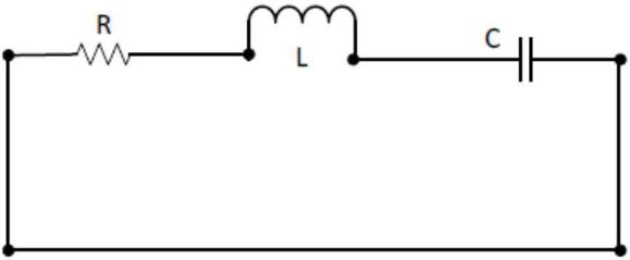
Figure 1 A source free series RLC circuit.
3 The Time Domain Behavioral Analysis
As stated above, the time domain behaviors of the system can be analyzed by study the influence of to , , , and . Noted that is of interested because it does not exist in the conventional biquadratic system but unique to the fractional one under consideration. In order to do perform the study, must be used. For simplicity, we let in (20). As a result, become
| (22) |
and can be simulated by assuming that rad/sec and which is a typical value [26], similarly to [23] as shown in Figure 2. Noted that this simulation and the rests have been performed by using MATHEMATICA. From Figure 2, a significantly different dynamic of from that of the previous dimensional consistency ignored step response [23] can be observed. In the following subsections, the influence of to , , , and will be respectively studied by assuming the above parameters.
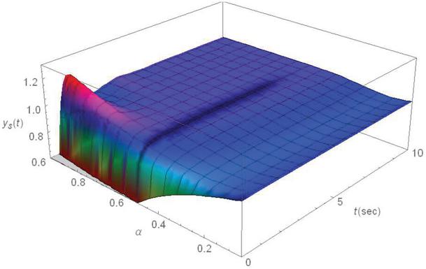
Figure 2 v.s. and .
3.1 The Influence of to
Before proceed further, it should be mentioned here that since if , if and the order of the system of our interested is 2, such system become a fractional order system with order ranged from 0 to 1 i.e., the maximum order is 1, and from 1 to 2 i.e., the maximum order is 2, when and respectively. Therefore, can be mathematically defined based on the following definitions
Definition 2: Let and be the response to of arbitrary linear 1st order system, can be defined as [19]
| (23) |
Definition 3: Let and be the response to s(t) of arbitrary linear 2nd order system, can be defined as [26]
| (24) |
As a result, we have
| (25) |
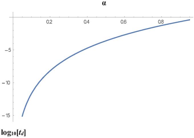
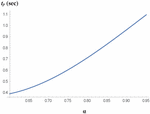
Figure 3 log v.s. .
By using (22), (25) and Newton-Raphson method [25], can be numerically determined in an iterative manner as follows
| (26) |
where (n) means n iteration of the Newton-Raphson method. Noted that can be given by
| (27) |
Therefore can be similarly given for both ranges of as follows
| (28) |
By using (26)–(28), can be simulated as a function of as depicted in Figure 3 which shows that log[t] is an increasing function of , however, the increasing rate is gradually lowered with higher . Therefore, t is also an increasing function of with such gradually lowered increasing rate. This implies that the rate of change of y(t) in the transient state is a decreasing function of according to the definition of t. It can also be stated that such decreasing in the rate of change at low values of is more significant than that at high values.
3.2 The Influence of to
According to [26], the definition of can be given in term of as follows.
Definition 4: Let , and , can be given by
| (29) |
As a result, can be numerically determined by using Newton-Raphson method as
| (30) |
where
| (31) | ||
| (32) | ||
| (33) | ||
| (34) | ||
| (35) | ||
| (36) |
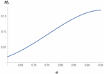
By using (30)–(36), can be simulated as a function of as depicted in Figure 3. Like t, it has been found that t is also an increasing function of with lower increasing rate when become higher as log does. Such lowering increasing rate of t become obvious when where under the assumed parameters as can be seen from Figure 4. Noted that different can be obtained if different sets of system parameters have been adopted. By the definition of , it can be pointed out that the rate of change of the magnitude of in its transient state from 10% to 90% of its steady state value is a decreasing function of where such decreasing is significant at .
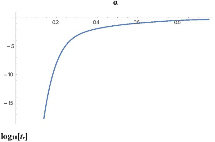
Figure 4 log] v.s. .
3.3 The Influence of to
Before we proceed further, the definition of should be given as follows.
Definition 5: Let where , can be defined as
| (37) |
Therefore, can be found numerically by using the Newton-Raphson method as
| (38) |
where
| (39) | |
| (40) |
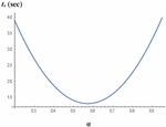
By using (38)–(40), we can simulate as a function of as depicted in Figure 5 which shows that the relationship between and displays a non-monotonic behavior. It has been found that is a decreasing function of i.e., , when and vice versa when . Noted that stands for the critical value of which yields the minimum value of i.e., . Therefore, and can be numerically determined by using (38)–(40) and the following equations
| (41) | |
| (42) |
Since the system begins to enter its steady state at , it has been found that the system with requires minimum time for being steady otherwise more time is needed. With (38)–(42), and can be found as and sec based on the assumed parameters stated above. Noted that different and can be obtained if different sets of system parameters have been adopted.
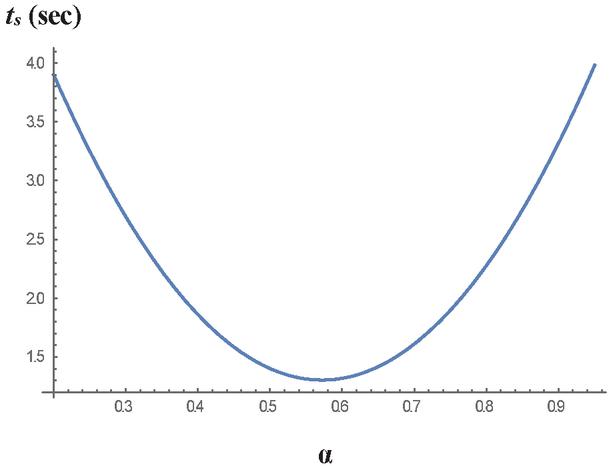
Figure 5 v.s. .
3.4 The Influence of to
Since reaches its peak at , it can be seen that
| (43) |
Therefore, can be determined by using the following equation
| (44) |
As a result, we can simulate the relationship between and as depicted in Figure 6 where only has been considered. This is because the overshoot of does exists if and only if as can be seen from Figure 1. It has been found that is an increasing function of and its rates of change is gradually increased with respected to . This implies that the of the system with reach its peak with faster speed if approaches 0.5 and become slower if approaches 1 where the decreasing in such speed when approaches 1 is more significant than that when approaches 0.5.
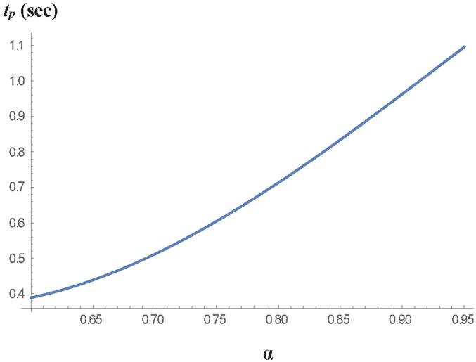
Figure 6 v.s. .
3.5 The Influence of to
At this point, the definition of will be given.
Definition 6: Let where , can be given by
| (45) |
By using this definition and numerically determined in the previous subsection, the relationship between and can be graphically portrayed as depicted in Figure 7 where only has been considered similarly to Figure 6.
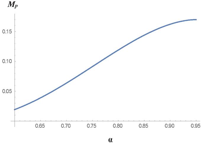
Figure 7 v.s. .
Table 1 Prominent features of the proposed research and related previous works
| Range | Considered | Dimensional | ||
| of | Physical | Consistency | ||
| Researches | System | Awareness | Remark | |
| The proposed research | 0–2 | Arbitrary | Included | Assuming arbitrary input and arbitrary . Application to electrical system has been shown. Influence of to , , , and has been studied. |
| [19] | 0–1 | Electrical | Not included | – |
| [20] | 0–1 | Electrical | Not included | – |
| [21] | 0–2 | Electrical | Included | Assuming zero input and zero . |
| [22] | 0–2 | Electrical | Not included | Assuming zero input and zero . |
| [23] | 0–2 | Arbitrary | Not included | Assuming arbitrary input and arbitrary . |
From Figure 7, it has been found that is also an increasing function of with the gradually increased rate of change with respected to . However, unlike that of , the rate of change of is lowered as approaches 1 and reach its maximum value i.e., , at certain value of i.e. . Based on the assumed parameters, and can be numerically determined by using (43)–(47) as and . It should be mentioned here that that different and can be obtained if different sets of system parameters have been adopted. Before we proceed to the conclusion, it is worthy to present a comparative summary of prominent features of this and related previous works as shown in Table 1.
| (46) | |
| (47) |
4 Conclusion
The dimensional consistency aware time domain analysis of fractional order biquadratic system with nonzero input and nonzero has been performed in this research. The fractional derivative terms of the system’s FDE which have been included, have been interpreted in the Caputo’s sense and the system’s response which employs a significantly different dynamic from its previous dimensional consistency ignored counterpart [23], has been analytically determined by solving such FDE. Also unlike [23], the application of the solution of system’s FDE on the electrical system has been shown and the influence of to , , and has been studied. The obtain results provide much insight to the fractional order biquadratic system with dimensional consistency awareness in a generic point of view regardless to the physical nature of any specific system. Therefore, this work has been found to be beneficial to the analysis/design of the fractional order systems and their related research areas.
Acknowledgement
The first author would like to acknowledge Prof. Manuel Ortigueira for his valuable advice.
References
[1] C.M.A. Pinto and A.R.M. Carvalho, ‘A latency fractional order model for HIV dynamics’, Journal of Computational and Applied Mathematics, vol. 312, pp. 240–256, 2017.
[2] C.M.A. Pinto and A.R.M. Carvalho, ‘The HIV/TB coinfection severity in the presence of TB multi-drug resistant strains’, Ecological Complexity, vol. 32, pp. 1–20, 2017
[3] P.D. Mandic’, T.B. Šcekara and M.P. Lazarevic’, “Dominant pole placement with fractional order PID controllers: D-decomposition approach’, ISA Transactions., vol. 67, pp. 76–86, 2017
[4] P.D. Mandic’, M.P. Lazarevic’ and T.B. Šcekara, ‘D-Decomposition technique for stabilization of furuta pendulum: Fractional approach’, Bulletin of the Polish Academy of Science: Technical Science, vol. 64, pp. 189–196, 2016.
[5] A. Allagui, T.J. Freeborn, A.S. Elwakil and B. Maundy, ‘Reevaluation of performance of electric double-layer capacitors from constant current charge/discharge and cyclic voltammetry’, Scientific Reports, vol. 6, 2016.
[6] T.J. Freeborn, A. Allagui and A. Elwakil, ‘Modelling supercapacitors leakage behaviour using a fractional-order model’, Proceedings of the European Conference on Circuit Theory and Design 2017, pp. 1–4, 2017.
[7] M. Cajic’, D. Karlicic’, and M. Lazarevic’, ‘Damped vibration of a nonlocal nanobeam resting on viscoelastic foundation: fractional derivative model with two retardation times and fractional parameters”, Meccanica, vol. 52, pp. 363–382, 2017.
[8] X. Wang, H. Qi, B. Yu, Z. Xiong and H. Xu, ‘Analytical and numerical study of electroosmotic slip flows of fractional second grade fluids’, Communications in Nonlinear Science and Numerical Simulation, vol. 50, pp. 77–87, 2017.
[9] Y. Jiang, H. Qi, H. Xu and X. Jiang, ‘Transient electroosmotic slip flow of fractional oldroyd-B fluids’, Microfluidics and Nanofluidics, vol. 21, 2017.
[10] A. Ullah, W. Chen and M.A. Khan, “A new variational approach for restoring images with multiplicative noise’, Computers & Mathematics with Applications, vol. 71, pp. 2034–2050, 2016.
[11] A. Ullah, W. Chen, S.G. Sun and M.A. Khan, “An efficient variational method for restoring images with combined additive and multiplicative noise,” International Journal of Applied and Computational Mathematics., vol. 3, pp. 1999–2019, 2017.
[12] N. Shrivastava and P. Varshney, ‘Efficacy of order reduction techniques in the analysis of fractional order systems’, Proceedings of the IEEE region 10 conference 2017, pp. 2967–2972, 2017.
[13] X. Yang, C. Li, T. Huang and Q. Song, ‘Mittag–Leffler stability analysis of nonlinear fractional-order systems with impulses’, Applied Mathematics and Computation., vol. 293, pp. 416–422, 2017.
[14] Y. Tang, N. Li, M. Liu, Y. Lu and W. Wang, ‘Identification of fractional-order systems with time delays using block pulse functions’, Mechanical Systems and Signal Processing, vol. 91, pp. 382–394, 2017.
[15] P.E. Jacob, S.M.M. Alavi, A. Mahdi, S.J. Payne and D.A. Howey, ‘Bayesian inference in non-Markovian state-space models with applications to battery fractional-order systems’, IEEE Transactions on Control Systems Technology, vol. 26, pp. 497–506, 2018.
[16] K. Leyden and B. Goodwine, ‘Fractional-order system identification for health monitoring’, Nonlinear Dynamics, vol. 92, pp. 1317–1334, 2018.
[17] S. Marir, M. Chadli and D. Bouagada, ‘New admissibility conditions for singular linear continuous-time fractional-order systems’, Journal of the Franklin Institute, vol. 354, pp. 752–766, 2017.
[18] Y. Wei, B. Du, S. Cheng and Y. Wang, ‘Fractional order systems time-optimal control and its application’, Journal of Optimization Theory and Applications, vol. 174, pp. 122–138, 2017.
[19] M. Guia, F. Gomez, and J. Rosales, ‘Analysis on the time and frequency domain for the RC electric circuit of fractional order’, Central European Journal of Physics, vol. 11, pp. 1366–1371, 2013.
[20] P. V. Shah, A. D. Patel, I. A. Salehbhai, and A. K. Shukla, ‘Analytic solution for the electric circuit model in fractional order’, Abstract and Applied Analysis, vol. 2014, 2014.
[21] F. Gomez, J. Rosales and M. Guia, ‘RLC electrical circuits of non-integer order’, Central European Journal of Physics, vol. 11, pp. 1361–1365, 2013.
[22] G.-A. J. Francisco, R.-G. Juan, G.-C. Manuel and R.-H. J. Roberto, ‘Fractional order RC and LC circuits’, Ingeniería Investigación y Tecnología, vol. 15, pp. 311–319, 2014.
[23] R. Banchuin and R. Chaisricharoen, ‘The FDE based time domain analysis of nonzero input/nonzero damping ratio fractional order biquadratic system’, Proceedings of the Joint International Conference on Digital Arts, Media and Technology with ECTI Northern Section Conference on Electrical, Electronics, Computer and Telecommunications Engineering, pp. 177–179, 2020.
[24] I. Podlubny, Fractional Differential Equations, vol. 198 of Mathematics in Science and Engineering: Academic Press, 1999.
[25] E. Kreyszig, Advanced Engineering Mathematics: John Wiley and Sons, 1999.
[26] B.C. Kuo and F. Golnaraghi, Automatic Control Systems: John Wiley and Sons, 2003.
[27] A. M. Mathai and H. J. Haubold, Special Functions for Applied Scientists: Springer, 2010.
Biographies

Rawid Banchuin received the B.Eng. degree in electrical engineering from Mahidol University, Bangkok, Thailand in 2000, the degree of M.Eng. in computer engineering and Ph.D. in electrical and computer engineering from King Mongkut’s University of Technology Thonburi, Bangkok, Thailand in 2003 and 2008 respectively. At the present, he is an associate professor of the Graduated School of Information Technology and Faculty of Engineering, Siam University, Bangkok, Thailand. His research areas include computation and mathematics in electrical and electronic engineering especially the fractional order and memristive devices, circuits, and systems.

Roungsan Chaisricharoen received B.Eng., M.Eng. and Ph.D. degrees from the department of computer engineering, King Mongkut’s University of Technology Thonburi, Bangkok, Thailand. He is an assistant professor at the school of information technology, Mae Fah Luang University, Chiang Rai, Thailand. His research areas include computational intelligence, analog circuits and devices, wireless networks, and optimization techniques.
Journal of Mobile Multimedia, Vol. 18_3, 789–806.
doi: 10.13052/jmm1550-4646.18316
© 2022 River Publishers