Optimizing MultiStack Parallel (MSP) Sorting Algorithm
Apisit Rattanatranurak and Surin Kittitornkun*
Dept. of Computer Engineering, School of Engineering, King Mongkut’s Institute of Technology Ladkrabang, Bangkok, Thailand
E-mail: apisit.ra@ssru.ac.th; surin.ki@kmitl.ac.th
*Corresponding author
Received 05 February 2021; Accepted 15 March 2021; Publication 18 June 2021
Abstract
Mobile smartphones/laptops are becoming much more powerful in terms of core count and memory capacity. Demanding games and parallel applications/algorithms can hopefully take advantages of the hardware. Our parallel MSPSort algorithm is one of those examples. However, MSPSort can be optimized and fine tuned even further to achieve its highest capabilities. To evaluate the effectiveness of MSPSort, two Linux systems are quad core ARM Cortex-A72 and 24-core AMD ThreadRipper R9-2920. It has been demonstrated that MSPSort is comparable to the well-known parallel standard template library sorting functions, i.e. Balanced QuickSort and Multiway MergeSort in various aspects such as run time and memory requirements.
Keywords: Partition, sort, multithread, OpenMP, optimize, synchronization.
1 Introduction
Smartphones’ CPUs are becoming multicore towards manycore to support a variety of multimedia applications. These mobile manycore CPUs are soon pervasive in both notebook and tablet computers. Therefore, basic computing algorithms shall be adapted to exploit that. Parallel sorting and data partitioning algorithms [5, 10, 9, 4] are based on the well known single-pivot Hoare’s algorithm [1]. It is also known as divide and conquer (D&Q) behavior of QuickSort.
Those algorithms can be broken into two phases: first level partition and partition & sort phases. The first phase is to compare and swap (C&S) between elements in parallel followed by a cleanup algorithm and sequential partition. The second phase recursively partitions two long subarrays and finally sorts the short ones in single thread.
The first level partition is the bottleneck of D&Q Hoare’s algorithm. This paper intends to tackle this problem with simple multithreading techniques while minimizing the unnecessary memory accesses. Based on our MultiStack Parallel Sorting (MSPSort) [7], we optimize and fine tune it further. Unlike other F&A parallel block-based QuickSort algorithms, MSPSort enforces data parallelism with left and right stacks of data blocks private to each thread. In addition, MSPSort is based on barrier synchronization to handle the classic skew pivot problem. However, the cleanup algorithm can be improved even more.
Our key contributions are as follows. First, the MSPPartition can be adaptive with respect to pivot value. It can adapt to the skew pivot such that fewer unnecessary recursive calls can be reduced while cleaning up the first level partition phase. Second, dynamic thread allocation can increase CPU threads to handle much longer subarrays due to imbalanced pivot. This can be beneficial to huge workloads on manycore CPUs. Third, the number of partitioning threads or CPU cores can be adjusted to support a wide variety of data types. As a result, fewer memory accesses are required instantaneously thus lower pressure to the memory hierarchy and power consumption. Workloads can be shared among partitioning threads where more free cores are available to sort subarrays in parallel. Our optimization methods are considered global because they can be effectively applied to any manycore CPU system.
We shall present the paper in the following order. Section 2 reviews related background and previous work of parallel D&Q sorting algorithms. The optimized and fine tuned MSPPartition and MSPSort are elaborated in Section 3. Consecutively, experiment results are compared on AMD R9-2920 and Raspberry Pi4 systems. The last section is Conclusions and Future Work.
2 Background & Related Work
This section consists of the following subsections, Standard Template Library Sequential/Parallel Sorting Functions and Anatomy of QuickSort Algorithms.
2.1 Standard Template Library Sequential/Parallel Sorting Functions
The Standard Template Library is a sequential sorting function for any data type. It is available in almost C compilers and prototyped as follow.
std::sort(RandomAccessIterator first,
          RandomAccessIterator last);
On the other end of spectrum, Balanced QuickSort or BQSort as mentioned earlier is a classic parallel/multithreaded quicksort algorithm [9]. Each thread assign blocks of data to compare&swap (C&S). A double ended queue of each thread holds the block boundaries and allows other threads to access from the second end. MultiWay Merge Sort or MWSort equally divides data into several subarrays and them [9]. Each subarray can be independently sorted in parallel and stored in a temporary array. It requires an extra space of memory with complexity of where is the data size. The Parallel MultiWay merging algorithm can yield the final sorted array. As a result, its run time is more stable compared with QuickSort algorithm.
2.2 Anatomy of Parallel QuickSort Algorithms
A number of parallel QuickSort algorithms have been proposed by [5, 10, 9, 4, 8, 2, 6] and ordered in time series. The recent one is called MSPSort by us [7]. All of them can be decomposed into two phases: first level partition and partition & sort phases. The First Level Partition Phase is the most challenging task for parallelization. It consists of parallel compare and swap (C&S) between elements followed by a cleanup algorithm and sequential partition. Due to its comparison-based nature and global memory accesses, it is limited by latency of address translation look aside buffer (TLB) and page table all the way to cache misses. It can be regarded as memory bound problem [8]. In addition, CPU hardware constraints for some basic data types such as floating-point numbers still exist. The second phase called Partition&Sort is to recursively partition two long subarrays while traversing the resulting tree of subarrays in multithread and to finally sort a shorter one by a single thread. Only major algorithms are summarized and compared with ours as follows.
In 1990, Heidelberger et al. [5] first proposed a block-based parallel partition algorithm on shared memory multiprocessor system. Reserving blocks of data to C&S must be synchronized using F&A instruction. Although it is initially in-place, the cleanup phase needs two extra buffers to keep track of elements’ indices to be swapped. The next phase can be accomplished using two global queues. The first queue keeps the longer subarrays to be partitioned in parallel with proportional number of processors. The second queue keeps shorter ones to be partitioned sequentially and consequently sorted. Several scheduling algorithms can be applied. The entire algorithm was simulated rather than implemented.
PQuickSort [10] was first implemented a block based parallel partition algorithm on a shared memory multiprocessor system in 2003. Each processor reserves a pair of blocks from both left and right sides to C&S data elements. The process continues to reserve one more fresh block from either on left or right side. All processors stop until no fresh block is available. Some unfinished blocks must be swapped to separate between the left and right finished blocks. The sequential partition eventually finishes the first-level partition. The next step assigns a number of processors proportional to subarrays’ sizes. A special stack is instantiated to store subarrays and shared among processors to partition and finally sorted them. Its run time complexity is where and are array size and number of CPU cores, respectively.
The BQSort [9] as mentioned earlier is also block based and recursive C&S. Fetch and add (F&A) synchronization is needed every time a data block is reserved. All threads stop when their C&S indices get closer within a block distance. Some data swaps must be carried out to prepare for the next recursive function call. Eventually, the sequential partition finishes the first level partition phase. Next, each thread’s local deque (double ended queue) can keep track of subarrays to be partitioned with shorter partition first (SPF) traversal. As a result, an idle thread can steal workload from the other end of a non-empty deque. Its run time complexity is .
A year later, Frias and Petit [4] used the same F&A synchronization scheme. However, they propose a new cleanup algorithm to avoid extra C&S. They apply a complete binary tree structure to keep track of the unfinished blocks so that they can be shared to balance workload on all CPU cores. Left data elements shall be swapped only with the right ones according to the leaves and finish up with sequential partition.
On the GPU (Graphic Processing Unit) computing side, these references [8, 2, 6] have all implemented parallel QuickSort algorithms based on NVIDIA GPUs using the CUDA Application Program Interface. One of the first papers implementing QuickSort on GPU was published by Sengupta, et al. in 2007 [8]. They are not in-place like CPU-based algorithms, Most of them consist of two phases. Phase I, the input array is divided into segments to fit the GPU local memory. Each section is assigned to a block of threads to compare against the pivot value to create a bit vector or C&S within a segment. The resulting two subsegments will be copied with synchronizations to form left and right subarrays in a buffer/shared memory. Phase II, either iterative or recursive partition continues and utilize different structures such as stack to keep track of the partitioned subarrays. Short subarrays are then sorted given a threshold.
Our MSPPartition/Sort [7] is a simple yet efficient block based C&S algorithm. Each thread has its own private left and right stacks of data blocks to enforce data parallelism without any F&A instruction. When either left or right stack of each thread runs out, the thread stops temporarily to synchronize with other threads. As a cleanup algorithm, recursive MSPPartition or a sequential one can be invoked while sacrificing C&S some elements again thanks to current smart branch prediction. In the next phase, combinations of breadth first and depth first traversals can partition to exploit cache locality and consequently them. No work stealing is necessary.
3 Optimized MSPSort Algorithm
Various factors of our MSPPartition can affect its performance such as block size, how to handle the leftover data, how to balance the workload between left and right partitions, etc.
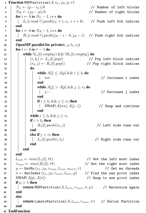
MSPPartition and MSPSort can be optimized and fine-tuned in the following aspects: block size, pivot value skew handling, number of threads in the first level, middle levels and final level of recursion. We can review and improve the MSPartition in pseudocode as shown in Algorithm 1.
Algorithm 1 Optimized Multi-Stack Partition Algorithm
3.1 Block Size
This MultiStack Parallel Partition function [7] The Recursive MultiStack Parallel Partition Phase can be decomposed of 2 steps: Parallel Stacked Blocks Partition Step and Unfinished Blocks Partition Step. The Parallel Stacked Blocks Partition Step divides an unsorted (sub)array , into left and right sides according to the pivot index . Each side is again divided into blocks of elements from both ends (Algorithm 1, line 4) where is a block size in KB (Kilo Bytes). Data blocks from left and right sides are assigned to threads in round robin to enforce data parallelism and avoid overlapping operations. Within its own assigned data blocks, each thread can C&S data just like Hoare’s algorithm. Therefore, there is no data race among threads.
3.2 Handling Pivot Value Skew in MSPPartition
To ideally balance workload and achieve maximum parallelism, each thread is initially assigned with about the same number of blocks. Each thread has its own private variables (local to each thread) and that are left and right indices within the current left and right blocks, respectively. In addition, two private variables, and are the boundaries of the current left and right blocks, respectively. The data from both sides are C&S within each iteration until either left or right index reaches its boundary (Alg.1, lines 15 to 24). Next, the current index pair either (,) or (,) of the latest unfinished block is pushed back to its corresponding stack (Alg.1, lines 27 and 30). In the next iteration, the boundaries of a new block and the unfinished one will be popped off to continue. This loop of each thread stops when either its left or right stack is empty (Alg.1, line 12).
After that, and of all threads, must be determined. The number of threads =GetMu() (Algorithm 1, line 36) corresponds to how many folds () is longer than and the current number of threads in Equation (1),
| (1) |
where
| (2) |
Next, the Unfinished Blocks Partition Step must take care of the pivot value skew issue. This step is the most critical part due to the random distribution of data and pivot value selection of . Earlier [7], the number of blocks on both sides must equal such that . However, pivot value skew can lead to the time consuming recursive calls to eventually partition the unfinished part. In this optimized MSPSort, the target index can be adaptive to the pivot value skew such that the number of recursions can be minimized. Therefore, it should be proportional to the finished (swapped) data elements as shown in Equation (3).
| (3) |
where () and () represent the lengths of left and right already swapped parts, respectively and () is the length of clean-up part.
In summary, the long unfinished part due to extreme pivot value skew can specify the number of threads of MSPPartition() and estimate the next pivot index from Equation (3) (Algorithm 1, line 40) in the Unfinished Blocks Partition Step. Otherwise, the Lomuto’s Partition [3] sequentially returns the pivot index (Algorithm 1, line 43).
3.3 Partition Thread Ratio
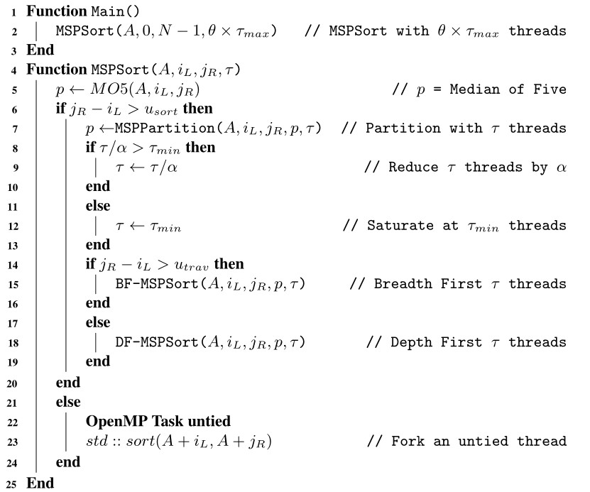
Based on our observations in the previous work [7], faster partition time can be also achieved at as well. As a result, the initial number of threads to partition can be parameterized to where is the Partition Thread Ratio. At line 2 of Algorithm 2, if , it shall relieve some pressure of the last level caches as well as the data TLBs where some partitioning threads must access data (memory) at various locations simultaneously.
Algorithm 2 Modified MSPSort Algorithm
3.4 Dynamic Thread Allocation
The Dynamic Thread Allocation consists of two independent parameters: Thread Divider and Thread Equalizer . The Thread Divider is between each recursive level. On the other hand, is the Thread Equalizer of the next recursion level to compensate with extremely skew pivot from the previous recursion. That means longer subarray on either left or right side may require more threads than its default number. If Thread Equalizer =ON, each side may get two different number of threads, and . Otherwise, =OFF, threads on both sides are equal, == in Equations (4) and (5).
| (4) |
and
| (5) |
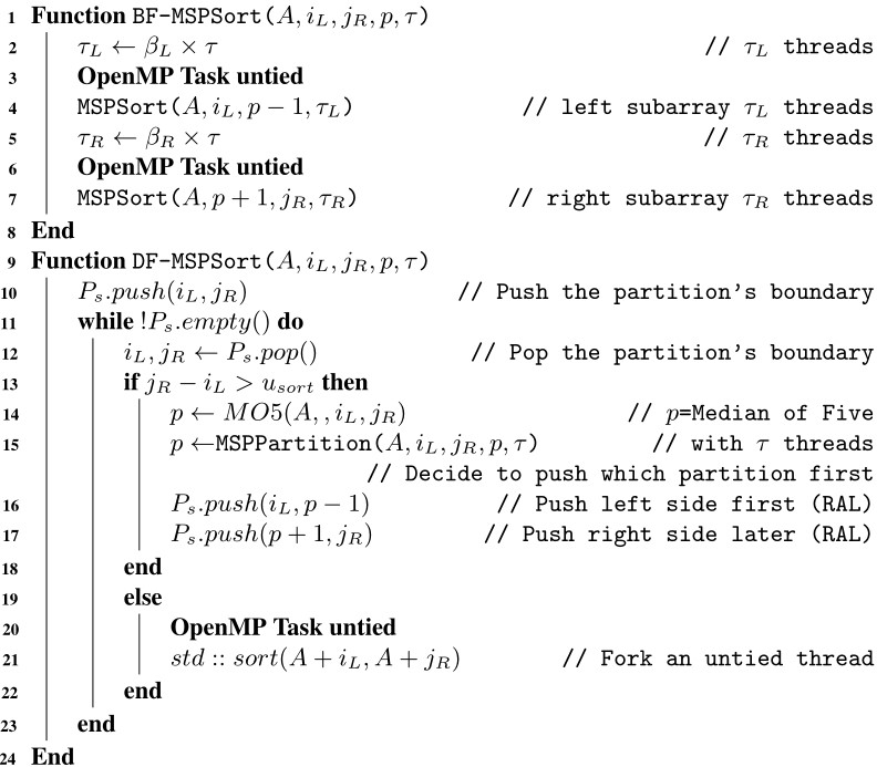
Algorithm 3 Breadth-First and Depth-First MSPSort
3.5 Depth First Traversal Algorithms
In the MSPSort() function, Median of Five function (Algorithm 2, line 5) selects a pivot index and swaps it to the middle of subarray . The MSPPartition() partititions the subarray with respect to the pivot index and finally returns it back (Algorithm 2, line 7). MSPSort() continues traversing the tree of subarrays with Breadth-First (Algorithm 2, line 15) by default. The details of BF-MSPSort() can be explored in Algorithm 3. It can be noticed that MSPSort() is invoked as two recursive untied OpenMP tasks (Algorithm 3, lines 3 and 7) corresponding to the left and right subarrays, respectively.
With the default BF traversal, any resulting shorter than subarray is sorted as an independent thread (Task) (Algorithm 2, line 23) using where , is Sorting Cutoff parameter, and corresponds to the data type (in bytes) to be sorted.
To achieve as high parallelism as possible, BF traversal is of the choice. Therefore, its unpredictable execution order can be due to various factors such as the subarray sizes, data TLB misses/page faults and branch/memory stalls. However, cache locality can be exploited at almost the deepest level of recursion. We have been implementing DF (Depth First) traversal algorithm in DF-MSPSort() function. Once the subarray () is shorter than elements (Algorithm 2, line 18), MSPSort switches to DF traversal where elements and is Traversal Cutoff in bytes. The pseudocode in Algorithm 3 illustrates RAL (Right Always) algorithm as an example.
There are two different approaches of BF-DF traversal, direction versus subarray size oriented. Both RAL and LAL (Left Always) are direction oriented. On the contrary, Longer Partition First (LPF) and Shorter Partition First (SPF) are size oriented. Several hybrid algorithms can be devised.
3.6 Minimum Threads
As the number of subarrays to be processed grows exponentially, deeper recursive level requires fewer threads. As a result, the number of software threads is reduced to (Algorithm 2, line 12) and kept at threads where is the minimum number of threads. In order to share CPU cores with other threads while maximizing parallelism, should be fine tuned as well.
4 Experiments, Results & Discussions
The experiments on two different Linux systems. Experiment parameters are listed and rationalized. Consecutively, the obtained results are elaborated and discussed.
Table 1 Specifications of multicore CPUs, KB: Kilo Bytes, MB: Mega Bytes
| CPU | Cortex A72 | ThreadRipper |
| Name | Pi4 | R9-2920 |
| Clock (GHz) | 1.5 | 3.50 |
| (cores) | 4 | 24 |
| RAM | 8GB | 64GB |
| Configuration | 18GB | 88GB |
| Technology | DDR4 | DDR4 |
| Frequency (MHz) | 2133 | 2400 |
| L1 I-Cache | KB 3 Way | KB 4 Way |
| L1 D-Cache | KB 2 Way | KB 8 Way |
| L2 Cache | 1024 KB 16 Way | KB 8 Way |
| L3 Cache | – | MB 16 Way |
| 64-bit OS | Raspberry Pi | Ubuntu |
| Version | Beta | 18.04 LTS |
| Kernel | 5.4.42-v8+ | 5.3.0-62-generic |
| G++ | 8.3.0 | 7.5.0 |
| OpenMP | 4.5 | 4.5 |
4.1 Experiment Setup
The fine-tuned MSPSort algorithm can be experimented on two totally different systems as listed in Table 1. They both run the same and G version. The number of cores is reported by Linux System Monitor. Moreover, these systems widely differ in terms of memory size, technology and configuration. Nonetheless, to compare between non-L3 cache CPU and L3-cache CPU cores. R9-2920 represents high-end mobile systems with high CPU core count, large RAM capacity and shared L3 caches. On the other hand, Raspberry Pi4 represents ordinary mobile systems with low core count, small RAM capacity and a shared L2 cache instead.
Table 2 Experiment parameters of , BF: Bread-First, DF: Depth-First, M=
| Parameters | Values |
| Algorithms | , , |
| Data Types | Uint32, Double |
| Random Dist | Uniform |
| GCC Optimization | O2 |
| Data size (Pi4) | 20M, 50M, 100M, 200M |
| Data size (R9) | 200M, 500M, 1000M, 2000M |
| Traversal | RAL, LAL, LPF, SPF |
| Block size | 32, 64, 128, 256 KB |
| Sorting Cutoff | 2, 4, 8, 16 MB |
| Traversal Cutoff | 8, 16, 32, 64 MB |
| Multiplier | 1, 2 |
| Minimum Thread | 2, 3 |
| Partition Thread Ratio | 0.67, 0.75, 0.8, 0.9 |
| Thread Divider | 4/3, 3/2, 2, 5/2 |
As listed in Table 2, the parameters on both Pi4 and R9-2920 systems are the same except N. The data types to be evaluated include Unsigned 32-bit integer (Uint32) and 64-bit double precision floating point numbers (Double). Only uniform distribution is evaluated. Each algorithm is compiled with -O2 flag to save experiment time. There are two sets of data size where ranges from 20M to 200M elements due to system RAM limit for Pi4 and 200M to 2000M for R9-2920.
As mentioned earlier, the block size , Sorting Cutoff and Traversal Cutoff are not parameterized with L3 Cache size 8MB. The block size is in order of KBs. Sorting Cutoff and Traversal Cutoff are in order of MBs as listed in Table 2. MSPSort can fork as many threads where the Multiplier = 1, 2. The minimum threads can be independent of hardware configuration, = 2, 3.
4.2 Key Performance Indicators (KPIs)
In this paper, some experiment results shall be normalized and compared based on these KPIs. They all represent time domain aspects of each sorting algorithm. Although lower and are better in terms of run time and stability, other statistics play important roles as well. We shall discuss the experiment results with respect to the following aspects.
4.2.1 Average run time () and run time per M ()
An omp_get_wtime() can be invoked twice just before and after running the algorithm to get accurate time stamps of each algorithm. The obtained time difference is the Run Time . Note that data array randomization and initialization as well as verification after are excluded.
The Average Run Time () can be normalized at Million elements and called Run Time per M (). Based on this, It is easy to compare at any data size for certain experiments. Furthermore, this normalized can be system independent and compared among several systems running the same algorithm.
4.2.2 Run time standard deviation and
Run Time Standard of Deviation () represents the stability of each algorithm due to the randomness of each workload. In addition, the normalized standard deviation () per Million elements can justify some parameters specially Block size .
4.2.3 Run time stability
In addition to arithmetic mean and standard deviation , the first, second and third quartiles are , and , respectively. The InterQuartile Range can be determined as =- for stability analyses. These statistics can specify how the Run Time distributes over 1000 trials.
4.2.4 Run time difference percentage:
To emphasize differences between MSPSort and other algorithms , this KPI is formulated as follows:
| (6) |
It is similar to Speedup equation. The positive values show how much MSPSort is faster in percentage. On the contrary, the negative values represent the opposite direction.
4.2.5 User-mode CPU utilization:
The amount of time that the CPU cores spending of a program can be measured in a virtual file /proc/stat. The CPU time consists of four major components: user, system, nice and idle modes. We are interested in user mode CPU utilization because the higher user-mode utilization , the more CPU is occupied by an algorithm. Other tasks shall be slowed down.
4.2.6 RAM utilization:
RAM can be limited due to cost constraints especially mobile platforms. The MaxResident is the maximum amount memory residing in RAM measured by /usr/bin/time Linux command in KiloBytes. Its man page is available online. Hence, the RAM Utilization percentage can be computed as follow.
| (7) |
The more memory (RAM) consumption compared to the workload size, the higher percentage. It is of concern to current mobile platforms especially smartphones/tablets due to RAM limitation.
4.3 Results & Discussions
In order to optimize and fine tune parameters of MSPSort effectively, we start with the bottom most parameters all the way up to the top ones.
4.3.1 BF-MSPSort vs block size
This subsection explains how we fine tune the block size for Uint32 and Double. Earlier [7] the block size MB which is about 80 KB. We start tuning to be multiples of 32 KB (L1 data cache) on both systems. It is expected that of larger data type as Double to be twice as big as that of Uint32 as show in Tables 3 and 4.
Table 3 and of BF-MSPSort, Uint32 and Double at various block sizes on Pi4 system after 100 trials
| Type | KPI (Sec.) | 20M | 50M | 100M | 200M |
| Uint32 | |||||
| =32KB | 0.6396 | 0.6615 | 0.7056 | 0.7332 | |
| 0.0079 | 0.0058 | 0.0139 | 0.0068 | ||
| =64KB | 0.6311 | 0.6627 | 0.6948 | 0.7359 | |
| 0.0112 | 0.0054 | 0.0071 | 0.0138 | ||
| =128KB | 0.7270 | 0.7616 | 0.7870 | 0.8334 | |
| 0.0206 | 0.0139 | 0.0090 | 0.0180 | ||
| Double | |||||
| =64KB | 1.0483 | 1.0978 | 1.1359 | 1.2004 | |
| 0.0250 | 0.0309 | 0.0193 | 0.0217 | ||
| =128KB | 1.0714 | 1.0887 | 1.1576 | 1.1986 | |
| 0.0203 | 0.0207 | 0.0383 | 0.0245 | ||
| =256KB | 1.0253 | 1.1047 | 1.1560 | 1.2007 | |
| 0.0115 | 0.0298 | 0.0379 | 0.0249 | ||
Table 4 and of BF-MSPSort, Uint32 and Double at various block sizes on R9-2920 system after 100 trials
| Type | KPI (Sec.) | 20M | 50M | 100M | 200M |
| Uint32 | |||||
| =32KB | 0.5762 | 0.6008 | 0.6244 | 0.6609 | |
| 0.05762 | 0.0172 | 0.0206 | 0.0285 | ||
| =64KB | 0.5774 | 0.6018 | 0.6250 | 0.6533 | |
| 0.0120 | 0.0147 | 0.0210 | 0.0141 | ||
| =128KB | 0.5753 | 0.5963 | 0.6247 | 0.6535 | |
| 0.0081 | 0.0141 | 0.0164 | 0.0156 | ||
| Double | |||||
| =64KB | 0.8775 | 0.9503 | 0.9937 | 1.0484 | |
| 0.0208 | 0.249 | 0.0194 | 0.0317 | ||
| =128KB | 0.8785 | 0.9473 | 0.9908 | 1.0325 | |
| 0.0154 | 0.224 | 0.0179 | 0.0382 | ||
| =256KB | 0.8776 | 0.9481 | 0.9827 | 1.0397 | |
| 0.0133 | 0.205 | 0.0265 | 0.0411 | ||
The selected values of are 64 KB for Uint32 and 128 KB for Double on both systems. The focus is on =200M and 2000M for Pi4 and R92920, respectively. It can be noticed that these values yield the optimal KPIs in terms of and as well as. The same reason for R9-2920 is and instead.
4.3.2 BF-MSPSort vs , ,
Given a fixed from the previous experiments, the next parameters, , and shall be investigated in BF-MSPSort. At the same time, we can learn how they interact to each other given the same data size . The top ( and ) tuples are listed in Table 5. It can be noticed that the whole run time is a trade off between partition time and sorting time.
Table 5 Top (, , , ) tuples with BF traversal for all ’s, after 20 Trials
| System | Pi4 | R9-2920 |
| Uint32 | (64kB, 4MB, 1, 2) | (64kB, 4MB, 2, 2) |
| (64kB, 4MB, 1, 3) | (64kB, 4MB, 1, 3) | |
| (64kB, 4MB, 2,2) | (64kB, 4MB, 1, 2) | |
| Double | (128kB, 8MB, 1, 2) | (128kB, 8MB, 1, 2) |
| (128kB, 8MB, 2, 2) | (128kB, 8MB, 1, 3) | |
| (128kB, 4MB, 1, 2) | (128kB, 8MB, 2, 2) | |
4.3.3 BF-MSPSort vs BF-DF algorithms
Given the top parameter tuple from BF-MSPSort listed on Table 5, we shall study how each traversal algorithm differs from one another. Earlier, must be configured to multiples of 8MB-L3 cache. In this optimized version, could be adjusted to be any number or as a function of problem size especially for huge ones. It turns out that MSPSort with RAL BF-DF traversal yields the best and for both systems and data types. Therefore, RAL is selected and thus called it RAL-MSPSort. Its final parameters are listed in Table 6.
Table 6 Selected top (, , , , ) tuples for RAL-MSPSort for all ’s, after 100 Trials
| System | Uint32 | Double |
| Pi4 | ||
| 20M-200M | (64KB, 4MB, 4MB, 1, 2) | (128KB, 8MB, 8MB, 1, 2) |
| R9-2920 | ||
| 200M | (64KB, 2MB, 8MB, 2, 2) | (128KB, 4MB, 8MB, 1, 2) |
| 500M | (64KB, 4MB, 16MB, 2, 2) | (128KB, 8MB, 16MB, 1, 2) |
| 1000M | (64KB, 8MB, 32MB, 2, 2) | (128KB, 8MB, 32MB, 1, 2) |
| 2000M | (64KB, 8MB, 32MB, 2, 2) | (128KB, 8MB, 64MB, 1, 2) |
RAL-MSPSort can yield the best Run Time statistics among all traversal algorithms, even though the BF execution order is similar to SPF algorithm. For both BF and SPF algorithms, shorter subarrays get partitioned done faster the resulting two subarrays can be enqueued sooner. This may not be good for last level cache on average.
With a single shared L2 cache, Pi4 system can be regarded as one-fourth of R9-2920 system. RAL-MSPSort still can yield better Run Time than BF traversal. especially when because MSPPartition() continues one more time resulting in two subarrays shorter than .
The cutoff may be different due to the data types and a wide variety of cache configurations especially mobile System on Chips. Some of them do not have L3 caches only L2 caches are available instead. In addition, some CPU cores are not identical such as ARM big.Little technology. Cache coherency may be an issue at the block as well as subarray boundaries. These boundaries can fall into the same cache block being accessed by two threads simultaneously.
4.3.4 RAL-MSPSort vs partition thread ratio
In this experiment, we shall explore how the number of threads running MSPPartition() affect the total Run Time . The maximum threads stays the same at only the initial partition threads is reduced to where . Based on parameters in Table 6, and of RAL-MSPSort at different are listed in Tables 7 and 8 for Pi4 and R9-2920 systems, respectively.
We can observe that Pi4 loses some performance on both data types as we apply . For R9-2920, of less than 1.00 mitigates that pressure thus yields faster Run Time. On the other hand, parallelism of Pi4 is limited by CPU cores rather than memory bottleneck.
On the contrary, R9-2920 gains significant performance only for Double at =0.8 not Uint32. Two major reasons are behind this phenomenon. Firstly, this is because Double data type is twice as big as Uint32 per data element. That means either L3 cache or RAM is twice as busy with Double data requests given the same amount of time as Uint32 data. Secondly, it may be due to floating-point hardware resource constraints as well. Note that R9-2920 is multithreaded CPU and actually a 12-core 24-thread CPU.
Table 7 and of MSPSort, RAL for Uint32 and Double at various sizes and Partition Thread Ratio on Pi4 system after 100 trials
| Alg. | KPI (Sec.) | 20M | 50M | 100M | 200M |
| Uint32 | |||||
| 1.2640 | 3.2878 | 6.8597 | 14.3510 | ||
| 0.0269 | 0.0357 | 0.0805 | 0.1368 | ||
| 1.2945 | 3.3392 | 6.8744 | 14.6111 | ||
| 0.0544 | 0.0578 | 0.0699 | 0.2899 | ||
| Double | |||||
| 2.1488 | 5.4478 | 11.4136 | 24.2979 | ||
| 0.0491 | 0.1079 | 0.2354 | 0.5938 | ||
| 2.1637 | 5.5548 | 11.5595 | 24.6450 | ||
| 0.0251 | 0.0666 | 0.1432 | 0.2352 | ||
Table 8 and of MSPSort, RAL for Uint32 and Double at various sizes and Partition Thread Ratio on R9-2920 system after 100 trials
| Alg. | KPI (Sec.) | 200M | 500M | 1000M | 2000M |
| Uint32 | |||||
| 1.1598 | 2.9678 | 6.2311 | 12.5458 | ||
| 0.0146 | 0.0245 | 0.1192 | 0.2564 | ||
| 1.1459 | 2.9757 | 6.1624 | 12.7117 | ||
| 0.0245 | 0.0847 | 0.2307 | 0.3633 | ||
| 1.1396 | 2.9329 | 6.2100 | 12.9028 | ||
| 0.0167 | 0.0388 | 0.1980 | 0.5081 | ||
| 1.1429 | 2.9468 | 6.2087 | 12.8381 | ||
| 0.0140 | 0.0524 | 0.2250 | 0.4650 | ||
| 1.1437 | 2.9518 | 6.2619 | 12.9881 | ||
| 0.0223 | 0.0566 | 0.3486 | 0.6049 | ||
| Double | |||||
| 1.7408 | 4.6700 | 9.6917 | 20.1682 | ||
| 0.0231 | 0.1736 | 0.2836 | 0.8512 | ||
| 1.7363 | 4.6454 | 9.5878 | 20.3231 | ||
| 0.0189 | 0.1460 | 0.2413 | 0.5916 | ||
| 1.7118 | 4.6077 | 9.5261 | 20.0296 | ||
| 0.0795 | 0.2034 | 0.4592 | 1.0444 | ||
| 1.7230 | 4.6286 | 9.5329 | 20.1099 | ||
| 0.0318 | 0.1658 | 0.4191 | 0.7131 | ||
| 1.7197 | 4.6421 | 9.6873 | 20.4310 | ||
| 0.0384 | 0.1327 | 0.3766 | 0.9811 | ||
4.3.5 RAL-MSPSort vs thread divider
The earlier MSPSort [7], the Thread Divider is always 2. The question may arise why in the next recursion is always divided by 2. Can other values be better than this? Thread Dividers =5/3, 3/2 and 4/3 that are less than 2 can result in more threads in the next recursion level. On the other hand, higher =5/2 can result in fewer threads. Based on the best parameters from the previous experiment, the effects of on Pi4 and R9-2920 systems are provided in Tables 9 and 10, respectively.
It can be observed that =2 yields the best results for Pi4 system and both types. On R9-2920 at Double =1000M and 2000M, the saddle points at =5/3 can be observed instead of =2. Hugh double workload may get benefit from Dynamic Thread Allocation. The effects of Thread Equalizer shall be presented in the last subsection. However, for simplicity =2 for both data types and all systems.
Table 9 and of MSPSort for Uint32 () and Double () at various sizes and on Pi4 system after 100 trials
| Alg. | KPI (Sec.) | 20M | 50M | 100M | 200M |
| Uint32 | |||||
| 1.2931 | 3.3368 | 6.9511 | 14.5192 | ||
| OFF | 0.0265 | 0.0568 | 0.0909 | 0.2386 | |
| 1.2931 | 3.3321 | 6.8597 | 14.4847 | ||
| OFF | 0.0297 | 0.0638 | 0.0976 | 0.2391 | |
| 1.2640 | 3.2878 | 6.8597 | 14.3510 | ||
| OFF | 0.0269 | 0.0357 | 0.0805 | 0.1368 | |
| 1.3303 | 3.4218 | 7.0489 | 14.7332 | ||
| OFF | 0.0723 | 0.0686 | 0.1065 | 0.1512 | |
| Double | |||||
| 2.1535 | 5.5741 | 11.5349 | 24.4927 | ||
| OFF | 0.0464 | 0.1681 | 0.1554 | 0.6259 | |
| 2.1488 | 5.4478 | 11.4136 | 24.2979 | ||
| OFF | 0.0491 | 0.1079 | 0.2354 | 0.5938 | |
| 2.2146 | 5.6488 | 11.6705 | 24.6764 | ||
| OFF | 0.0479 | 0.1959 | 0.3204 | 0.5461 | |
Table 10 and of MSPSort for Uint32 () and Double () at various sizes and on R9-2920 system after 100 trials
| Alg. | KPI (Sec.) | 200M | 500M | 1000M | 2000M |
| Uint32 | |||||
| 1.1603 | 2.9786 | 6.2968 | 12.7600 | ||
| OFF | 0.0167 | 0.0388 | 0.1980 | 0.5081 | |
| 1.1598 | 2.9678 | 6.2311 | 12.5458 | ||
| OFF | 0.0146 | 0.0245 | 0.1192 | 0.2564 | |
| 1.1740 | 3.0219 | 6.4761 | 13.0133 | ||
| OFF | 0.0245 | 0.0869 | 0.3986 | 0.7027 | |
| Double | |||||
| 1.7356 | 4.6483 | 9.6046 | 20.1066 | ||
| OFF | 0.0557 | 0.1152 | 0.2038 | 0.5079 | |
| 1.7255 | 4.6356 | 9.4302 | 19.8885 | ||
| OFF | 0.0725 | 0.1871 | 0.5151 | 0.9203 | |
| 1.7118 | 4.6077 | 9.5261 | 20.0296 | ||
| OFF | 0.0795 | 0.2034 | 0.4592 | 1.0444 | |
| 1.7889 | 4.8657 | 10.2009 | 21.4310 | ||
| OFF | 0.0724 | 0.3059 | 0.6525 | 1.7900 | |
Table 11 KPIs (Seconds) of of RAL-MSPSort vs BQSort vs MWSort for Uint32 () and Double () at various sizes on Pi4 system after 1000 trials, =OFF
| Alg. | KPI (Sec.) | 20M | 50M | 100M | 200M | 200M |
| Uint32 | =ON | |||||
| MSPSort | 1.2949 | 3.3129 | 6.9138 | 14.4948 | 14.6631 | |
| 1.2749 | 3.2883 | 6.8673 | 14.4120 | 14.5390 | ||
| 1.2732 | 3.2866 | 6.8607 | 14.3877 | 14.4783 | ||
| 1.2539 | 3.2622 | 6.8136 | 14.3117 | 14.3709 | ||
| 0.0410 | 0.0507 | 0.1002 | 0.1831 | 0.2922 | ||
| 0.0306 | 0.0374 | 0.0875 | 0.1626 | 0.2313 | ||
| BQSort | 1.2814 | 3.4008 | 7.1837 | 14.9355 | ||
| 1.2682 | 3.3726 | 7.1146 | 14.8235 | |||
| 1.2640 | 3.3663 | 7.0907 | 14.8122 | |||
| 1.2482 | 3.3389 | 7.0259 | 14.6850 | |||
| 0.0332 | 0.0619 | 0.1578 | 0.2505 | |||
| 0.0327 | 0.0480 | 0.1268 | 0.1986 | |||
| MWSort | 1.2517 | 3.2947 | 6.9192 | 14.6352 | ||
| 1.2401 | 3.2739 | 6.8760 | 14.5602 | |||
| 1.2354 | 3.2678 | 6.8708 | 14.5445 | |||
| 1.2243 | 3.2469 | 6.8253 | 14.4635 | |||
| 0.0274 | 0.0478 | 0.0939 | 0.1717 | |||
| 0.0243 | 0.0400 | 0.0693 | 0.1453 | |||
| Double | =ON | |||||
| MSPSort | 2.1275 | 5.5136 | 11.6239 | 24.6005 | 24.6358 | |
| 2.0899 | 5.4371 | 11.4603 | 24.2545 | 24.3857 | ||
| 2.0806 | 5.4507 | 11.4952 | 24.2736 | 24.3834 | ||
| 2.0452 | 5.3733 | 11.2931 | 23.8399 | 24.1348 | ||
| 0.0823 | 0.1403 | 0.3308 | 0.7606 | 0.5010 | ||
| 0.0610 | 0.1154 | 0.2571 | 0.5938 | 0.4926 | ||
| BQSort | 2.0836 | 5.5412 | 11.7007 | 24.8755 | ||
| 2.0442 | 5.4775 | 11.5933 | 24.6479 | |||
| 2.0424 | 5.4627 | 11.5666 | 24.6200 | |||
| 1.9991 | 5.4014 | 11.4318 | 24.3610 | |||
| 0.0845 | 0.1398 | 0.2689 | 0.5145 | |||
| 0.0540 | 0.1134 | 0.2541 | 0.4409 | |||
| MWSort | 1.9794 | 5.3865 | 11.6665 | 24.9317 | ||
| 1.9667 | 5.3554 | 11.5684 | 24.8053 | |||
| 1.9639 | 5.3343 | 11.5659 | 24.6787 | |||
| 1.9504 | 5.2840 | 11.4709 | 24.4965 | |||
| 0.0290 | 0.1025 | 0.1956 | 0.4352 | |||
| 0.0249 | 0.0826 | 0.1848 | 0.5598 | |||
Table 12 KPIs (Seconds) of of RAL-MSPSort vs BQSort vs MWSort for Uint32 and Double at various sizes on R9-2920 system after 1000 trials, =OFF
| Alg. | KPI (Sec.) | 200M | 500M | 1000M | 2000M | 2000M |
| Uint32 | =ON | |||||
| MSPSort | 1.1615 | 3.0147 | 6.2208 | 12.8731 | 12.7956 | |
| 1.1532 | 2.9871 | 6.1665 | 12.8096 | 12.6881 | ||
| 1.1511 | 2.9720 | 6.1285 | 12.7004 | 12.6646 | ||
| 1.1416 | 2.9378 | 6.0565 | 12.5842 | 12.5497 | ||
| 0.0199 | 0.0765 | 0.1743 | 0.2889 | 0.2459 | ||
| 0.0194 | 0.0245 | 0.1192 | 0.2564 | 0.1976 | ||
| BQSort | 1.2849 | 3.3515 | 6.9910 | 14.8314 | ||
| 1.2641 | 3.3027 | 6.8910 | 14.4880 | |||
| 1.2608 | 3.2872 | 6.8587 | 14.3754 | |||
| 1.2366 | 3.2211 | 6.7273 | 13.9707 | |||
| 0.0483 | 0.1304 | 0.2637 | 0.8607 | |||
| 0.0398 | 0.1266 | 0.2883 | 0.7737 | |||
| MWSort | 1.2690 | 3.1965 | 6.9421 | 14.6856 | ||
| 1.2605 | 3.1748 | 6.7743 | 14.4544 | |||
| 1.2482 | 3.1424 | 6.8500 | 14.5239 | |||
| 1.2368 | 3.1253 | 6.4225 | 14.3433 | |||
| 0.0322 | 0.0712 | 0.5196 | 0.3423 | |||
| 0.0351 | 0.0748 | 0.2940 | 0.3672 | |||
| Double | =ON | |||||
| MSPSort | 1.7501 | 4.6861 | 9.7268 | 20.5472 | 20.2142 | |
| 1.7335 | 4.6198 | 9.6218 | 20.3233 | 20.0028 | ||
| 1.7302 | 4.6215 | 9.5645 | 20.2944 | 19.9662 | ||
| 1.7137 | 4.5675 | 9.4322 | 20.0442 | 19.7528 | ||
| 0.0364 | 0.1186 | 0.2946 | 0.5030 | 0.4614 | ||
| 0.0328 | 0.1771 | 0.3427 | 0.6693 | 0.4716 | ||
| BQSort | 1.8262 | 4.8709 | 10.2529 | 21.6878 | ||
| 1.7977 | 4.7990 | 10.0812 | 21.3060 | |||
| 1.7821 | 4.7602 | 10.0035 | 21.0510 | |||
| 1.7562 | 4.6768 | 9.8058 | 20.6554 | |||
| 0.0700 | 0.1941 | 0.4471 | 1.0324 | |||
| 0.0593 | 0.1729 | 0.4180 | 1.0467 | |||
| MWSort | 1.5818 | 4.0025 | 8.9359 | 18.2426 | ||
| 1.5700 | 4.0276 | 8.7317 | 18.0441 | |||
| 1.5659 | 3.9595 | 8.8775 | 18.0956 | |||
| 1.5542 | 3.9384 | 8.7910 | 17.9187 | |||
| 0.0276 | 0.0641 | 0.1449 | 0.3239 | |||
| 0.0244 | 0.1598 | 0.3418 | 0.4057 | |||
4.3.6 RAL-MSPSort: final results vs. thread equalizer
Once the parameters are finalized (=OFF), the RAL-MSPSort is evaluated again at 1000 trials to get more stable results and benchmarked with BQSort and MWSort. Run time statistics of all sorting algorithm of Pi4 and R9-2920 are enumerated in Tables 11 and 12, respectively. On Pi4 system and 100M, all of both data types of all algorithms are similar. At workload =200M, RAL-MSPSort’s to are the best in all categories. On R9-2920, RAL-MSPSort performs extremely fast on Uint32 data. However, MWSort is still the fastest of Double data type.
For run time stability analyses of both systems, and can be of interests. The and of RAL-MSPSort are mostly lower than those of BQSort and MWSort for both data types. It can be concluded that RAL-MSPSort is consistently stable on both low-end and high-end mobile systems.
The Thread Equalizer is only switched ON for =200M and =2000M on Pi4 and R9-2920, respectively. The experiment results are augmented to the final ones at the right most column. Left and right Thread Equalizers and correspond to Equations (4) and (5), respectively. Due to the off balanced pivot selection, the much longer subarray is to be partitioned further with more threads. It can be noticed at =200M that Pi4 system loses both and . This can be due to small number of =4 cores. However, R9-2920 system has shown that =ON can handle both huge Uint32 and Double workloads, i.e. =2000M well. Their Run Time statistics are much better than that of =OFF.
4.4 Other Percentage KPIs
Other KPIs in percentage are summarized of Pi4 and R9-2920 systems in Tables 13 and 14, respectively. The Percentages of Run Time Difference of MSPSort become positive values at larger workloads on both algorithms and both systems. The overhead of MSPPartition is well justified with Uint32 data type at larger workloads. The only exception is at MWSort on R9-2920 system that can localize data to the CPU cores.
From average user mode CPU utilization point of view, RAL-MSPSort incurs lower values than BQSort but a bit higher than MWSort. That means operations of stacks to interleave C&S data within blocks can be effective yet similar to the original Hoare’s. Unlike BQSort that can steal workloads from other deques, RAL-MSPSort relies on thread scheduling of OpenMP to balance the CPU Utilization. Therefore, Some CPU cores can be available to other urgent tasks instead of synchronizing.
Table 13 KPIs (%) of of RAL-MSPSort vs BQSort vs MWSort for Uint32 and Double at various sizes on Pi4 system after 1000 trials, =OFF
| Alg. | KPI (%) | 20M | 50M | 100M | 200M |
| Uint32 | |||||
| MSPSort | 92.19 | 95.89 | 97.17 | 97.77 | |
| 103.79 | 101.67 | 100.85 | 100.54 | ||
| BQSort | -0.53 | 2.56 | 3.60 | 2.86 | |
| 98.28 | 98.64 | 98.81 | 98.91 | ||
| 103.99 | 101.60 | 100.80 | 100.40 | ||
| MWSort | -2.73 | -0.44 | 0.13 | 1.03 | |
| 93.33 | 93.89 | 94.26 | 94.52 | ||
| 203.83 | 201.54 | 200.78 | 200.40 | ||
| Double | |||||
| MSPSort | 93.38 | 96.28 | 97.22 | 97.67 | |
| 100.83 | 100.79 | 100.43 | 100.26 | ||
| BQSort | -2.19 | 0.74 | 1.16 | 1.62 | |
| 97.93 | 98.25 | 98.41 | 98.53 | ||
| 101.97 | 100.79 | 100.40 | 100.20 | ||
| MWSort | -5.90 | -1.50 | 0.94 | 2.27 | |
| 90.95 | 91.78 | 92.32 | 92.75 | ||
| 201.92 | 200.78 | 200.39 | 200.19 | ||
Table 14 KPIs (%) of of RAL-MSPSort vs BQSort vs MWSort for Uint32 and Double at various sizes on R9-2920 system after 1000 trials, =OFF
| Alg. | KPI (%) | 200M | 500M | 1000M | 2000M |
| Uint32 | |||||
| MSPSort | 90.73 | 93.34 | 94.02 | 94.04 | |
| 100.56 | 100.38 | 100.26 | 100.21 | ||
| BQSort | 9.62 | 10.57 | 11.75 | 13.10 | |
| 94.30 | 94.80 | 94.38 | 91.03 | ||
| 100.57 | 100.23 | 100.12 | 100.06 | ||
| MWSort | 9.30 | 6.28 | 9.86 | 12.84 | |
| 89.39 | 91.31 | 88.72 | 85.93 | ||
| 200.55 | 200.22 | 200.11 | 200.05 | ||
| Double | |||||
| MSPSort | 87.32 | 87.31 | 86.92 | 87.95 | |
| 100.31 | 100.25 | 100.20 | 100.18 | ||
| BQSort | 3.70 | 3.88 | 4.77 | 4.84 | |
| 92.06 | 89.51 | 86.67 | 87.42 | ||
| 100.29 | 100.12 | 100.06 | 100.03 | ||
| MWSort | -9.43 | -12.82 | -9.25 | -11.21 | |
| 86.31 | 86.81 | 82.99 | 82.75 | ||
| 200.24 | 200.11 | 200.05 | 200.03 | ||
The extra RAM Utilization percentage over 100% is considered overhead. The bigger workload, the smaller overhead is for all algorithms. This overhead stems from the data structures to handle parallel scheduling operations. Given the same problem size , Double data type incurs less amount of overhead percentage. RAL-MSPSort and BQSort need similar amount of RAM for both Uint32 and Double. However, MWSort requires double the RAM spaces as the /usr/bin/time command reports. It can be due to fact that the MultiWay Parallel Merge function [9] needs an extra buffer with space complexity as shown 200% in Tables 13 and 14. It is crucial on mobile platforms that are RAM limited.
5 Conclusions & Future work
Our fine-tuned MSPSort has been proved that its performance is comparable to the Standard Template Library parallel sorting algorithms, i.e. BQSort and MWSort. The comparison is carried out on two mobile-equivalent Linux systems, i.e. quad core ARM Cortex A72 on Raspberry Pi4 and 24-core AMD ThreadRipper representing low-end and high-end systems. The key performance indicators include run time statistics, user-mode CPU utilization and memory (RAM) utilization.
For further improvements, the current stack implementation shall be investigated and replaced with other structures such as deque. Our MSPPartition shall be applied to solve other fundamental problems such as parallel median, minimum and maximum value selections. In addition, a combination of Shortest Partition First and RAL traversal algorithms shall be explored to gain even more cache locality.
References
[1] Charles Antony and Richard Hoare. Quicksort. ACM, 4:321, 1962.
[2] Daniel Cederman and Philippas Tsigas. Gpu-quicksort: A practical quicksort algorithm for graphics processors. J. Exp. Algorithmics, 14:4:1.4–4:1.24, January 2010.
[3] Thomas H. Cormen, Charles E. Leiserson, Ronald L. Rivest, and Clifford Stein. Introduction to Algorithms, Third Edition. The MIT Press, 3rd edition, 2009.
[4] Leonor Frias and Jordi Petit. Parallel Partition Revisited, volume 5038 of Lecture Notes in Computer Science. Springer Berlin Heidelberg, 2008.
[5] Philip Heidelberger, Alan Norton, and John T. Robinson. Parallel quicksort using fetch-and-add. IEEE Transactions on Computers, 39(1):847–857, January 1990.
[6] Emanuele Manca, Andrea Manconi, Alessandro Orro, Giuliano Armano, and Luciano Milanesi. Cuda-quicksort: an improved gpu-based implementation of quicksort. Concurrency and computation: practice and experience, 28(1):21–43, 2016.
[7] Apisit Rattanatranurak and Surin Kittitornkun. A multistack parallel (msp) partition algorithm applied to sorting. Journal of Mobile Multimedia, pages 293–316, 2020.
[8] Shubhabrata Sengupta, Mark Harris, Yao Zhang, and John D. Owens. Scan Primitives for GPU Computing. In Mark Segal and Timo Aila, editors, SIGGRAPH/Eurographics Workshop on Graphics Hardware. The Eurographics Association, 2007.
[9] Johannes Singler, Peter Sanders, and Felix Putze. Mcstl : The multi-core standard template library. Euro-Par 2007 Parallel Processing. Springer Berlin Heidelberg, pages 682–694, 2007.
[10] Philippas Tsigas and Yi Zhang. A simple, fast parallel implementation of quicksort and its performance evaluation on sun enterprise 10000. In 11th Euromicro Conference on Parallel Distributed and Network based Processing (PDP 2003), pages 372–381, Genoa, Italy, February 5th-7th 2003.
Biographies

Apisit Rattanatranurak received his M.Eng. and B.Eng. degrees in Computer Engineering from King Mongkut’s Insitute of Technology Ladkrabang (KMITL), Bangkok, Thailand. Now, he is pursuing a doctoral degree at the School of Engineering, KMITL. His research interest is in the area of parallel programming, computing on multi-core CPU and GPU on Linux/Unix system.

Surin Kittitornkun received his Ph.D. and M.S. degrees in Computer Engineering from University of Wisconsin-Madison, USA. Currently, he is an Assistant Professor at School of Engineering, King Mongkut’s Insitute of Technology Ladkrabang (KMITL), Bangkok, Thailand. His research interests include parallel algorithms, mobile/high performance computing and computer architecture.
Journal of Mobile Multimedia, Vol. 17_4, 723–748.
doi: 10.13052/jmm1550-4646.17412
© 2021 River Publishers