Enhanced Road Lane Detection Facing Sun Glare

Mohammed El Amine Moumene^* and Mohamed Benkedadra

Department of Mathematics and Computer Science, faculty of exact sciences and informatics, University Abdelhamid Ibn Badis Mostaganem, Algeria

E-mail: elamine.moumene@univ-mosta.dz; mohamedbenkedadra@univ-mosta.dz

*Corresponding Author

Received 04 March 2021; Accepted 04 April 2021; Publication 18 June 2021

Abstract

There are several studies on road lane detection but very few address adverse conditions for acquisition such as sun glare. Loss of details in underexposed images captured facing a low sun leads to misleading road lane detection. High Dynamic Range Imaging methods are used to acquire most details in such scenes. Unfortunately, these techniques are heavy on computations and therefore unsuitable for real time road lane detection. In this paper, we propose a machine learning solution that avoids High Dynamic Range Imaging computations that are the radiance map estimation, tone-mapping algorithms and quality measures calculation. We train a neural network on a High Dynamic Range Imaging dataset. The resulting model produces suitable images for road lane detection facing sun glare, in real time. Subjective and objective comparisons with the most popular High Dynamic Range Imaging method, Mertens Algorithm, are conducted to prove the effectiveness of the proposed Neural Network. The delivered images demonstrated an improvement in road lane detection.

Keywords: Road lane detection, high dynamic range imaging, neural network.

1 Introduction to Lane Detection Facing Sun Glare

The camera is one of the most important sensors fitted on an Autonomous vehicle. It is commonly used for road lane detection, which is responsible for the decision making of steering the vehicle. Detecting painted road markings on successive images delivered by a camera mounted in front of the vehicle is a solution that attracted several studies. Two main modules are necessary for lane detection: feature extraction then model fitting. Lane marks are generally bright bands on a darker tarmac. Based on this strong assumption, analyzing image intensity variations is the most adopted method for lane marks detection. Canny or Sobel operators are widely used [1–3]. Once candidate lane marking points are extracted, a geometrical model is fitted. Mostly a straight line is used as a model since lane marks appear straight in zones that are near the vehicle, even in curved roads. Therefore, the estimation of straight line parameters is fast. Hough Transform is widely used to fit lines [4–6].

The lane detection algorithm needs to be reliable in extreme conditions. Unfortunately, sensors may find difficulties in some adverse scenarios and may produce misleading data for decision making, which will decrease the safety level of the Autonomous Vehicle. When the camera is facing the sun, the flare will cause an increase in the scene’s dynamic range. This High Dynamic Range of intensities is usually not supported by the camera’s capturing sensor, causing it to focus on a sub dynamic range. As a result, areas with lighting intensities outside of that sub-range are not going to be captured correctly, resulting in loss of details. Figure1.1 represents a scene recorded from a moving vehicle. When the lane detection steps mentioned above are applied on delivered images, none of the painted marks can be detected on the auto exposure. In this case, the needed details of the painting marks can be found in an overexposed image. The camera is unable to capture all scene details in one single image because of the High Dynamic Range. During this scene, the driver is dazzled. It is at this very moment that a lane departure warning system is needed most.

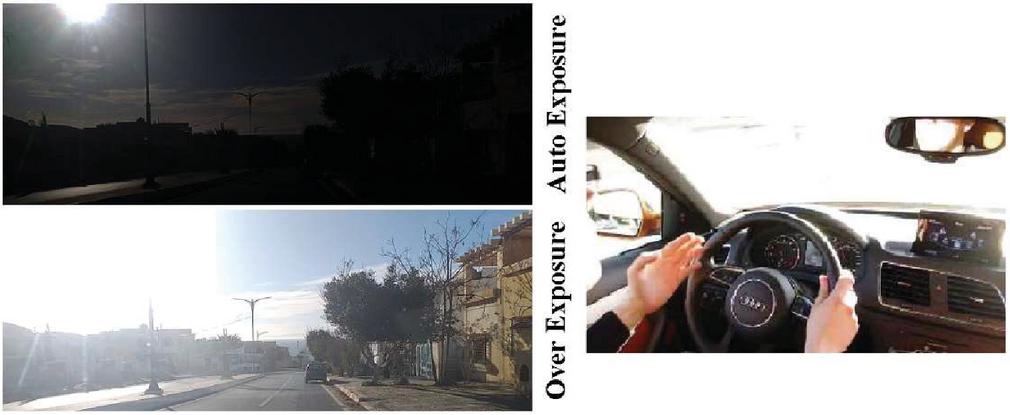
Figure 1 Extreme lighting condition: sun glare (high dynamic range scene).

There is a set of methods that is used in order to correctly capture high dynamic range scenes with minimum detail loss, into either high dynamic or low dynamic range image formats. The high dynamic range imaging pipeline starts from the capturing phase. Exposure Bracketing is the process of taking multiple pictures of the same scene with different Exposure Values (EVs). The idea is to cover the high dynamic range scene (all scene details) with many sub ranges. A sub range (an exposure) captures details present in an area having certain lighting conditions (Figure 2).

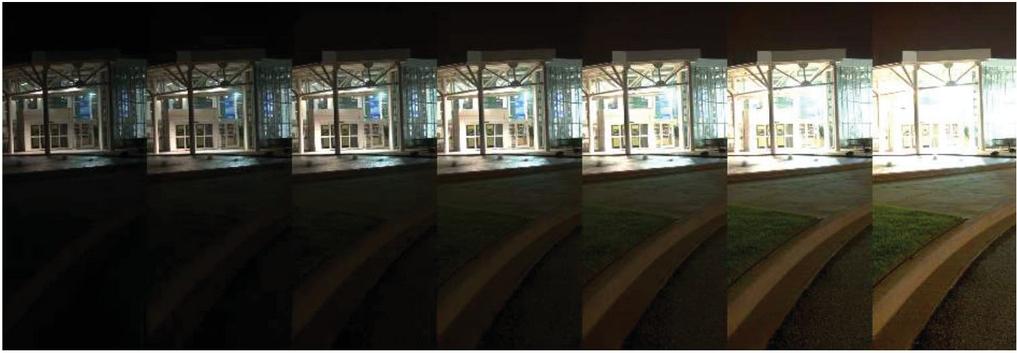
Figure 2 Exposure Bracketing (EB) from $-$ 3EV to $+$ 3EV ( $+$ 1EV per picture left to right).

Once exposures are captured, two approaches can be used to perform High Dynamic Range Imaging (HDRI). The first method is simply known as HDR [7, 8]. It starts with a Camera Response Function (CRF) calibration, followed by an image fusion process to create a 32bitHDR image. That image will later be converted, using a tone mapping operator [9], into an 8bit more detailed LDR image, which is easier to work with and facilitates display. CRF, image fusion, and tone mapping, are what define the HDR method from Exposure Fusion (EF). This second approach is easier to conduct, since it simply merges multiple LDR images with different EVs into a single enhanced LDR image. This is done in a single process, without going through the inconvenience of CRF estimation, HDR image creation and tone mapping operator application. Furthermore, Exposure Fusion (EF) which was made popular by Tom Mertens is taken advantage of [10]. The idea is to calculate different quality measures on each pixel across the bracketing to produce weight maps. Those maps are used to construct a single detailed image fusion. Calculated quality measures are Contrast, Saturation and Well-Exposedness.

Performing High Dynamic Range Imaging is time consuming. The 32 Bits HDR image reconstruction and tone mapping are both taxing on system resources. Exposure fusion might seem like a better and faster approach, but it also depends on many time-consuming steps (calculating quality measures for each pixel of the bracketing). Those methods are, therefore, not suitable for real time applications such as lane departure warning systems. Fei Kou et al. [11] use averaging between exposures as a fusion to reduce the processing time for a lane departure warning system. This oversimplified fusion produces images with less contrast and a loss of scene details. In the works [12] and [13], two techniques are proposed to leave out the weighting operations of a conventional exposure fusion. The first technique used a collection of images composed of inputs and their fusions to define generalized fusion weights. The second technique adopted a histogram segmentation phase that detects shadows and highlights intermediate regions of the bracketing before constructing image fusion with those segmented regions. However, the two methods rely on only two exposures (underexposed and overexposed images) as input for the fusion, which is not sufficient when facing a dazzling sun (greater High Dynamic Range).

In this paper we present a real time exposure fusion method that takes three exposures as input and delivers suitable images facing a dazzling sun. We train a neural network starting from a collection of exposures and their generated fusion by Tom Mertens Algorithm [10]. The resulting model is used to merge exposures directly. The usual HDRI computations as radiance map creation, tone mapping or quality measures estimation are avoided. The proposed Neural Network Exposure Fusion (NNEF) can be tested directly on our website and the implementation is available on GitHub [15]. The remainder of this paper is presented in three sections: Section two introduces the proposed neural network model and the training process. In section three we compare delivered image fusion by the NN with the original Mertens algorithm and we demonstrate how it enhances lane detection application facing a bright sun. Finally, the fourth section presents the conclusion.

2 Neural Network For Enhanced Images Facing Sun Glare

As seen before, HDRI is time consuming and not suitable for real time applications such as lane departure warning systems. In the proposed Supervised Machine learning HDRI, we feed a Neural Network with different samples of HDR scenes. Each sample is a set of LDR exposures, taken using automatic EB and labeled with an already created Exposure Fusion image using the Mertens Algorithm [10]. The model is supposed to find out how to produce a more detailed LDR scene representation, starting from any exposure bracketing.

We consider three different RGB exposures as inputs (Over-exposed, Normal exposure and Under-exposed) for the fusion. A vector of nine values (values on the RGB channels) can represent every pixel from the resulting image. The idea is to estimate the RGB values for each pixel in the fusion, based on the RGB values of that pixel position across the different exposures, and without performing any quality measures. The Neural Network model is given a 9 $\times$ 1 vector, representing the different RGB values, in the three different exposures, at a specific pixel position. Consequently, it would provide a 3 $\times$ 1 vector containing the RGB values of the pixel at the same position in the fusion.

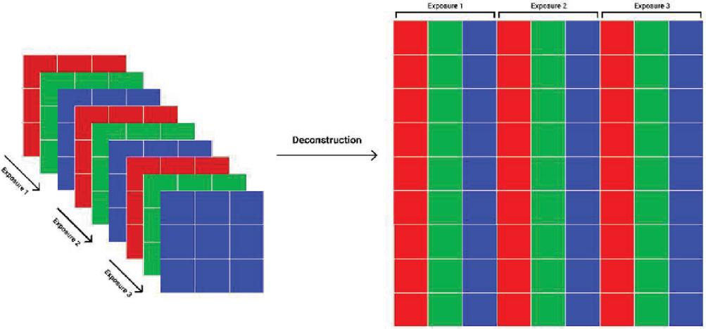
Figure 3 Preparing the different exposures for the fusion model training.

The deconstruction phase shown in Figure 3 transforms the three exposures into a data table that can be fed to the model. After running each row through the model, we get another table where each row represents RGB values of a specific pixel in the fusion. A Construction Phase is then performed where the resulting table is transformed into an actual fusion image. The architecture of the Neural Network (NN) was selected through an exhaustive examination of multiple network configurations. It was obtained by changing layers, different numbers of nodes and using different functions. Figure 4 represents the NN design that results in the best outputs.

The NN takes nine values as an input. Since we are working in the RGB color space, the values are in the [0-255] range. In order to have a stable solution, we chose to normalize the values by using MINAMX Normalization (Equation (1)). This transforms all values to the [0–1] range.

X_{i} = \frac{X_{i} - M i n}{M a x - M i n} = \frac{X_{i} - 0}{255 - 0} = \frac{X_{i}}{255}

(1)

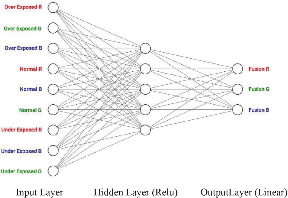
Figure 4 Exposure fusion neural network (EFNN).

Hidden layers in NNs add a level of complexity and detail, that allows for extracting and transforming the input information, into data that increases the probability of the production of a greatly improved quality output. We chose very simple functions as activations for the hidden layers’ neurons. One function being a normal linear activation function. Another one being the popular ReLU (rectified linear unit) activation function. A function that only provides positive values for outputs, as RGB values are always positive. We have also tried sigmoid activation since we are working in the [0–1] interval. This, however, did not present acceptable results.

Since we chose to normalize the input values to a [0–1] interval, we went with sigmoid activation for the output nodes in order to have an output that is also in the [0–1] interval. Multiplication by 255 is performed to get the real RGB values. It turned out that using sigmoid produced unacceptable results in certain extreme lighting conditions. Therefore, we choose a normal linear function.

The model requires a dataset where each sample is a set of two vectors. The first vector is an input example represented as a 9 $\times$ 1 vector containing three RGB values of the same pixel position across three different exposures. The second one is the correct output for an input example represented as a $3 \times 1$ vector and contains the RGB value for that specific pixel position in the Mertens image fusion. The used dataset contains hundreds of millions of samples, with pixels from different types of scenes and various dynamic ranges. Indoor, outdoor, day and night scenes are provided. This extreme data variation would assure that the model wouldn’t be biased towards specific kinds of scenes or specific sub dynamic ranges. The used image dataset was constructed from the HDR photographic survey database [14], where each scene is defined by three exposures (Overexposed, Normal and Underexposed) and labeled with a fusion using Mertens Algorithm. After the deconstruction phase, over 200 million samples are shuffled and saved into files.

Creating a machine learning model is a tedious process. That is because it requires training many different models with different parameters in order to hopefully find the best possible one. Using Keras, a high level API for the Tensorflow library, we are able to implement, test, and modify different models quickly. We begin by reading the RGB dataset as explained above. The dataset contains over 200 million samples, with each sample containing $9 + 3 = 12$ RGB values. In Python, each RGB value [0–255] takes at most 2 bytes of space. Therefore, at least 2.4 GB of RAM is required for loading the dataset. Normalization calls for the use of floating point values, which withholds a considerable amount of space. As Python uses 8 bytes per float number, it allocates 19.2 GB of RAM. The machine learning process was conducted on 25 GB of RAM.

We divide the dataset into 2 parts: 80% of samples are used in the training phase, while 20% are later used to test the model. Using Keras, it was possible to implement the previously seen Exposure Fusion Neural Network (EFNN) in just a few lines of code, as seen below:

model = tf.keras.Sequential()
model.add(
                    tf.keras.layers.Dense( 5, input_shape =(9,), activation=”relu”)
)
Model.add(
                    Tf.keras.layers.Dense(3,activation = “linear”)
                    )

To start the training phase, we pass the normalized data, the size of the batches and the epoch to the adaptive moment estimation algorithm [15], using the next lines of code:

model .fit( train_data , train_labels,
                  epochs = 10,
                  batch_size = 256 ,
                  callbacks =[ checkpoint ] )

The entire NNEF implementation is available in GitHub [16]. A summary of the proposed method is shown in Figure 5. Once the proposed Neural Network is trained, we can use it to predict exposure fusion. The real time exposure fusion algorithm starts by reading three exposures. Then, the previously explained deconstruction phase is performed using the function sample.create_np_data (). The resulting deconstructed data is normalized then used with the trained model to generate the fusion vector. This prediction is performed using the function model.predict(). Finally, the construction phase reshapes the fusion vector into an image containing most details of the exposure bracketing.

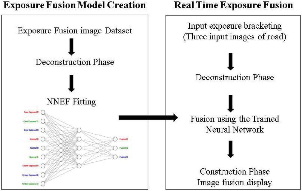
Figure 5 Exposure fusion neural network training and the real time image fusion algorithm.

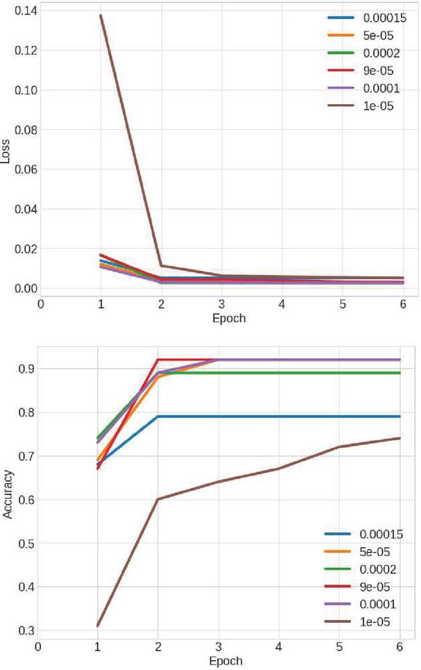
Figure 6 Effects of different learning rates on loss and accuracy.

3 Results and Comparisons

Learning occurs when the entire dataset is passed forward (from input to output) through the model. Then, a backward pass is done from output to input where the weights are recalculated and updated. After training multiple models of different rates, we settle a learning rate between 0.00005 and 0.0001. It is perceivable in Figure 6 that learning rates in that interval are better. In Figure 7 we can see that a batch number of 256 returns the best accuracy while decreasing the loss. Training the model for extended periods increases the chances of overfitting. Training for longer times causes poor quality in lighting and shadows.

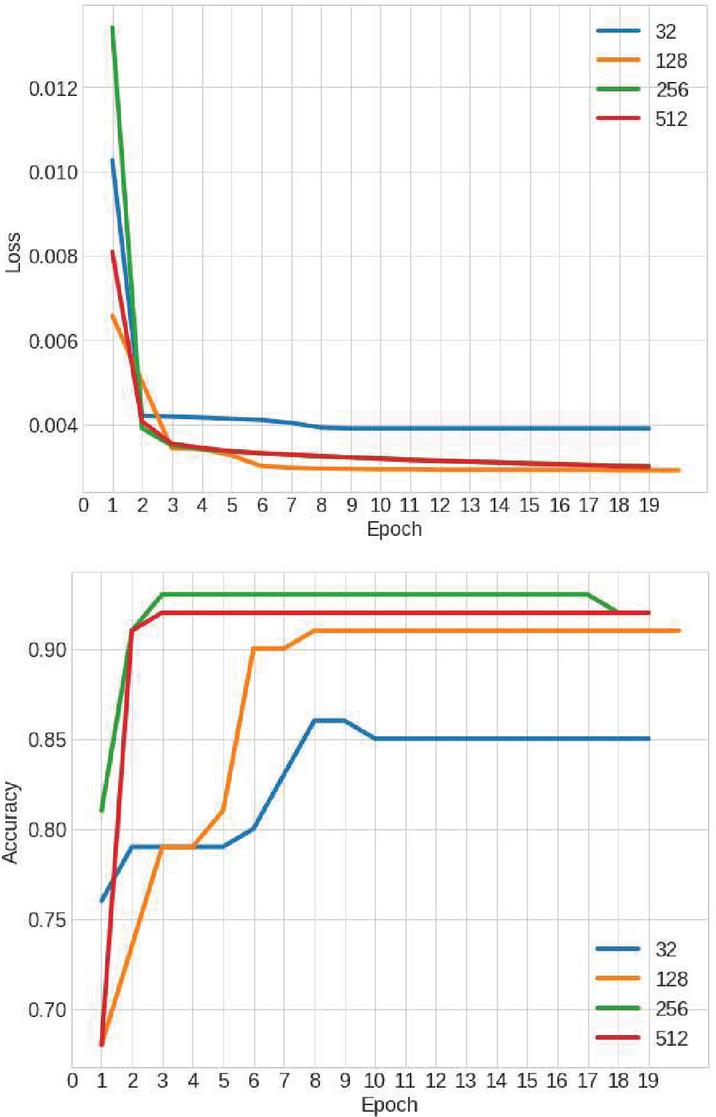
Figure 7 Effect of different batch sizes on loss and accuracy.

Figure 8 EFNN (Up) vs Mertens EF (Bottom).

After the training phase, the obtained Neural Network allowed us to fuse any unseen exposure bracketing. As in Figure 8, the model mimics the Mertens exposure fusion algorithm. We use three quality measures for objective comparisons between the proposed NNEF and Mertens Algorithm. We compute the mutual information [17]. Then, we calculate the color difference using CIEDE2000 and contrast difference. Ground truth images are constructed manually with the best parts of inputs and without deformation of pixels values. Results presented in Table 1 show that the proposed NNEF provides generally similar results as the Mertens algorithm in terms of mutual information, in CIEDE2000 and contrast di?erence. From a time-consumption perspective, EFNN is much faster with an average of 150 ms of processing time per frame. In fact, it approximately requires a tenth of the time needed by the widely used Mertens EF algorithm. The processing time improvement is even more impactful at high resolutions.

Table 1 Objective comparisons between the proposed neural network exposure fusion and Mertens algorithm

	Proposed Method	Mertens Algorithm
Contrast Difference	1.15	1.09
Color Difference	1.21	1.33
Mutual Information	5.61	4.78
Average CPU Time	1.6 Sec	0.13 Sec

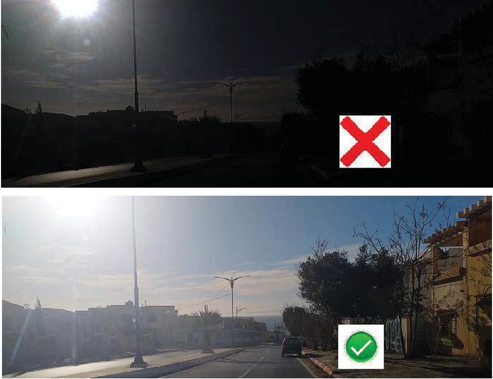
Figure 9 Road lane marks facing sun glare. auto-exposure (above), neural network exposure fusion (bottom).

We construct an image dataset composed of 2413 frames acquired from a moving vehicle facing sun glare. The images were captured using both camera’s auto exposure and the proposed NNEF. As seen in Figure 9, the proposed method provides suitable images facing sun glare. Auto exposed images are dim when facing a low sun and lots of road details are lost. For comparison, we implement two different methods based on the most adopted technique for road lane detection. The first one is based on the least square line fitting and RANSAC algorithm to reduce the effect of outliers [18]. The second one is based on Hough Transform; it is similar to [19]. The performance of the lane detection methods is quantified by True Positive Rate and False Detection Rate:

TPR	$= \frac{Detected lines}{Total number of lines}$
FDR	$= \frac{False Positives}{Detected lines + False Positives}$

As shown in Table 2, when using auto-exposed images as input for the road lane detection algorithms, a true positive rate less than 8 % is obtained by both methods and an important false detection rate is returned. On the other hand, when the proposed NNEF is performed before the same road lane detection algorithms, the true positive rate is enhanced and the false detection rate is reduced.

Table 2 Road Lane detection performance facing sun glare. Auto exposure vs Proposed NNEF

Method	TPR	PDR
Auto exposure + Hough Transform	5%	35%
Proposed NNEF + Hough Transform	67%	11%
Auto exposure + RANSAC	8%	49%
Proposed NNEF + RANSAC	51%	17%

4 Conclusion and Perspectives

In this paper, we are taking a problem rarely addressed in the literature, which is the detection of a road lane facing sun glare. As a solution, we propose a real time Neural Network based exposure fusion. The trained neural network on an HDRI dataset allows fusion of any non-seen exposure bracketing on a very small processing time compared to usual techniques. This supervised learning approach helps avoid tedious High Dynamic Range Imaging computations while preserving competitive image quality. The proposed technique is suitable for driver assistance systems such as a lane departure warning system. The delivered images using NNEF demonstrated consequent improvement on road lane true positive rate and reduction of false detection rate.

References

[1] S. Yenikaya, G. Yenikaya, and E. Duven, “Keeping the vehicle on the road a survey on on-road lane detection systems,” acm Computing Surveys (CSUR), vol. 46, October 2013.

[2] P. Wu, C. Chang, and C. H. Lin, “Lane-mark extraction for automobiles under complex conditions,” Pattern Recognition, vol. 47, p. 27562767, August 2014.

[3] B. Yu and A. Jain, “Lane boundary detection using a multiresolution hough transform,” International Conference on Image Processing, vol. 2, 1997, pp. 748–751.

[4] A. B. Hillel, R. Lerner, D. Levi, and G. Raz, “Recent progress in road and lane detection: a survey,” Machine Vision and Applications, vol. 25, pp. 727–745, April 2014.

[5] C. Yuan, H. Chen, J. Liu, D. Zhu and Y. Xu, “Robust Lane Detection for Complicated Road Environment Based on Normal Map,” in ieee Access, vol. 6, pp. 49679–49689, 2018.

[6] J. A. Christopher Rose, Jordan Britt and D. Bevly, “An integrated vehicle navigation system utilizing lane-detection and lateral position estimation systems in difficult environments for GPS,” ieee transactions on intelligent transport systems, vol. 15, pp. 2615–2628, 2014.

[7] P. E. Debevec and J. Malik, “Recovering high dynamic range radiance maps from photographs,” in ACM siggraph 2008 classes, pp. 1–10, 2008.

[8] C. Aguerrebere, J. Delon, Y. Gousseau, and P. Musé, “Best algorithms for HDR image generation. a study of performance bounds,” SIAM Journal on Imaging Sciences, vol. 7, no. 1, pp. 1–34, 2014.

[9] Y. Salih, W. bt. Md-Esa, A. S. Malik, and N. Saad, “Tone mapping of HDR images: A review,” 4th International Conference on Intelligent and Advanced Systems (ICIAS2012), vol. 1, pp. 368–373, June 2012.

[10] T. Mertens, J. Kautz and F. Van Reeth, “Exposure Fusion,” 15th Pacific Conference on Computer Graphics and Applications (PG’07), Maui, HI, 2007, pp. 382–390.

[11] F. Kou, W. Chen, J. Wang and Z. Zhao, “A lane boundary detection method based on high dynamic range image,” IEEE 10th International Conference on Industrial Informatics, Beijing, 2012, pp. 21–25.

[12] M. E. Moumene, R. Nourine and D. Ziou, “Generalized Exposure Fusion Weights Estimation,” 2014 Canadian Conference on Computer and Robot Vision, Montreal, QC, 2014, pp. 71–76.

[13] M. E. Moumene, R. Nourine and D. Ziou, “Fast Exposure Fusion Based on Histograms Segmentation,” International Conference on Image and Signal Processing, France, 2014, pp. 367–374.

[14] M. D. Fairchild, “The HDR photographic survey dataset (HDRPS),” 2017: http://markfairchild.org/HDR.html.

[15] Diederik P. Kingma, Jimmy Ba, “Adam: A Method for Stochastic Optimization”, 3rd International Conference on Learning Representations, 2015.

[16] M.E.Moumene, M. Benkedadra, “Exposure fusion Neural Network”, 2021: https://efnn.ml.

[17] Guihong, Dali and Pingfan, Y., “Information measure for performance of image fusion”, Electronics Letters 28(7):313–315. 2002.

[18] Amol Borkar, Monson Hayes, Matk T. Smith, “A novel lane detection system with efficient ground truth generation,” IEEE transactions on intelligent transport systems, vol. 13, pp. 365–374, 2012.

[19] A. Lopez, J. Serrat, C. Canero, F. Lumbreras, and T. Graf, “Robust lane markings detection and road geometry computation,” International Journal of Automotive Technology, vol. 11, pp. 395–407, 2010.

Biographies

Mohammed El Amine Moumene received a computer engineering degree from Mostaganem University in 2010 and a Ph.D. degree in computer vision from Oran 1 University in 2018. He is currently working as an assistant professor at the Department of Mathematics and Computer Science in Mostaganem university. His research areas include computer vision, machine learning and data mining.

Mohamed Benkedadra received a bachelor degree in Computer Systems from Mostaganem university in 2018, then a Master degree in Information Systems Engineering from the same university in 2020. He is currently working as the CTO of a start-up and a freelance contractor software engineer. He is specialized in web and crawling technologies, machine learning based computer vision.