Examination of the Non-Orthogonal Multiple Access System Using Long Short Memory Based Deep Neural Network
Ravi Shankar1,*, T. V. Ramana2, Preeti Singh3, Sandeep Gupta4 and Haider Mehraj5
1Madanapalle Institute of Technology & Science, Madanapalle, India
2Chitkara University school of Engineering and Technology, Chitkara University, Himachal Pradesh, India
3UIET, CSJM University, Kanpur, India
4JECRC University, Jaipur, Rajasthan, India
5Baba Ghulam Shah Badshah University, Rajouri, J&K, India
E-mail: ravi.mrce@gmail.com; jecsandeep@gmail.com
*Corresponding Author
Received 04 March 2021; Accepted 22 September 2021; Publication 29 October 2021
Abstract
This paper investigates deep learning (DL) non-orthogonal multiple access (NOMA) receivers based on long short-term memory (LSTM) under Rayleigh fading channel circumstances. The performance comparison between the DL NOMA detector and the traditional NOMA method is established, and results have shown that the DL-based NOMA detector performance is far better in comparison with conventional NOMA detectors. Simulation curves are compared with the performance of the DL detector in terms of minimum mean square estimate (MMSE) and least square error (LSE) estimate, taking all realistic circumstances, except the cyclic prefix (CP), and clipping distortion into account. The simulation curves demonstrate that the performance of the DL-based detector is exceptionally good when it equals 1 when the noise signal ratio (SNR) is more than 15 dB, assuming that the DL method is more resilient to clipping distortion.
Keywords: NOMA, LSTM, CP, SNR, Rayleigh fading.
1 Introduction
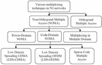
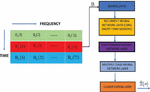
Emerging fifth generation (5G) NOMA networks provide a significant increase in end-to-end reliability, massive connectivity, higher bandwidth, reduced latency, and higher bandwidth than fourth generation (4G) wireless networks. The schematic representation of the NOMA network and NOMA schemes are given in Figures 1 and 2, respectively [1–3].
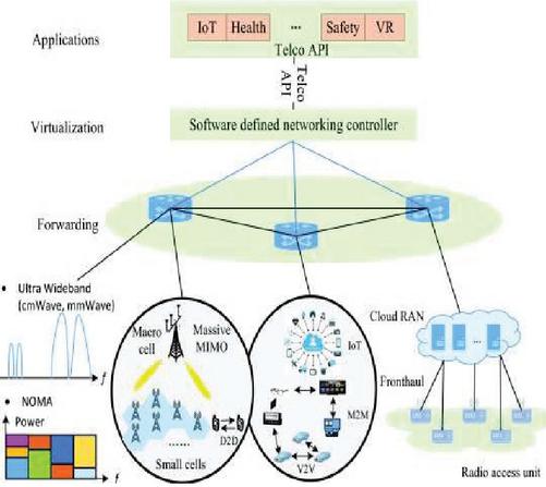
Figure 1 Schematic representation of the NOMA network [1–3].
NOMA delivers a better throughput than orthogonal frequency division multiple access (OFDMA) [4] technique for time varying channel fading conditions. Because the cell-center 5G connecting devices is spectrally efficient, it advantages more from being able to employ double channel capacity, even if the transmitted power is very low. The basic concept behind NOMA is to employ the power and code domain multiplexing technique for multiple access (MA), rather than the code/time/frequency as used in earlier generations of 5G wireless networks. Because the NOMA allows several users to use the same resource, such systems can be subject to interference. When compared to traditional systems, NOMA systems support cognitive, cooperative, and visible light communications paradigms.
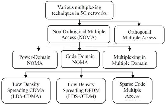
Figure 2 A classification of the various multiplexing mechanisms used in NOMA networks in 5G networks [2].

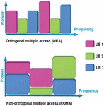
Figure 3 The schematic representation of the OMA and NOMA scheme.
While the 5G NOMA technology offers numerous advantages, more connecting devices, with this technology can be more secure and have data privacy with improved capability for information sensing. As a result, a variety of security issues ranging from the physical to the application levels must be addressed to design a strong, efficient, and effective system using this technology. The comparison between the NOMA and orthogonal multiple access (OMA) is given in Figure 3 [5–7]. Due to the presence of the inter symbol interference (ISI), the bit error rate (BER) performance of the system significantly decreases. The orthogonal frequency division multiplexing (OFDM) technique significantly degrades the ISI. The spectral efficiency will be considerably improved by combining NOMA with OFDM. One of the main advantages of the MMSE estimator is that it needs no prior knowledge of the CSI.
By combining channel and noise variance data, the LSE estimator is outperformed by the MMSE estimator. The use of the LSTM based DL algorithm in NOMA network has recently sparked a lot of attention. Signal detection, modulation recognition, CSI feedback, and channel estimation are some of the approaches provided for DL-based NOMA networks to improve the performance of various conventional algorithms. Deep neural networks (DNNs) have demonstrated notable results in complicated machine learning (ML) tasks such as wireless communication or cooperative NOMA networks. The authors in work [8] investigate the MIMO-OFDM network with adaptive modulation and coding using the convolutional neural network (CNN) based DL method. The primary goal of this study is to maximize channel capacity while keeping the BER limitation in mind. The real time propagation constraints such as carrier frequency offset, imperfect timing synchronization, and imperfect CSI is considered in this work. The estimated CSI and the noise variance are considered input features to the CNN. The advantage of the work is that it does not require the complex feature selection and it predicts the appropriate coding and modulation scheme also it successfully learns the MIMO-OFDM channel properly.
In [9], the authors explored the recognition of signal modulation in the OFDM network, and it is the key to the detection and recovery of signals. The authors examine the detection of OFDM signals based on the DL Signal modulation that is paired with a CNN trained on phase and quadrature data samples. However, the CNN based DL approach is slower due to the maxpool operation. Also, the training process will take more time when the number of layers are increasing, and the computer does not consist good graphics processing unit (GPU). In the papers [10–14], Recurrent neural network (RNN) detection for magnetic recording channels with ISI was examined by the authors. The authors train bidirectional gated units (bi-GRUs) recurring units to recover ISI input from noisy channel output sequences. When applied to continuously stream information, the network performance has been assessed.
The main detection technique used in conventional NOMA networks is the SIC technique. In both the uplink (U/L) and the downlink (D/L) NOMA OFDM network, the SIC technique is used extensively. Since the SIC technique leads to error propagation due to the receiver complexity. In the works [15, 16], the authors have investigated the DL based channel detection techniques that will detect the channel coefficients automatically.
In this work, DL based detection technique is proposed for the NOMA-OFDM over the Rayleigh fading channel conditions. The proposed DL NOMA-OFDM detector perfectly decodes and estimates the originally transmitted user data.
➢ The proposed technique improves the BER performance and decreases the overhead of the reference signal and this increases the D/L NOMA system’s data rate and end-to-end reliability.
➢ One of the advantages of the proposed technique is that it can process the conventional NOMA data directly instead of designing the SIC-based detector.
➢ The advantage of the DNNs based detector is that it can handle big data applications.
➢ Furthermore, the NOMA detector is characterized by DNN, which is jointly performing signal detection and channel estimation.
The following is how this paper is structured. Section 2 covers the fundamentals of DL, as well as the OFDM architecture and NOMA network explanation. Section 3 provides a detailed explanation of the DL NOMA receiver as well as model training. Section 4 will show preliminary simulation results, and Section 5 will provide conclusions.
2 System Model
2.1 DL Basics
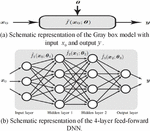
By examining the essential aspects and properties of the input signals, DL algorithms deliver greater performance than standard man-made algorithms. DNNs can learn the dynamic properties of natural information signals like audio and picture data files and utilize them for classification and decision-making. In general, the generated signals in a wireless communication system are man-made, therefore modeling of the fading channel is extremely straightforward, as it is obtaining the near Shannon’s capacity limits. There are various issues with wireless networking on the physical layer that we already know how to address optimally, such as employing well-established detection, optimization theory, estimation, and wireless communication networks. Nonetheless, there are important functional concerns where, for example, it is difficult to obtain adequate answers due to a lack of acceptable models or methods. Deep structured learning, abbreviated as DL, is an ML methodology based on representation learning and a component of the artificial neural network (ANN). ML algorithms are divided into three types: unsupervised, supervised, and semi-supervised algorithms. DNNs, RNNs, LSTMs, and CNNs are employed in domains such as natural language processing, social network filtering, bioinformatics, audio recognition, and speech recognition, with results comparable to, and in some cases exceeding, the performance of human-made algorithms. ANNs are based on the notion of human brain function or, in a broader sense, biological systems and signal processing applications. However, the structure of ANNs differs greatly from that of the human brain. Human brains are extremely complex, dynamic, and they are living organisms and dynamic. Instead of the human brain, ANNs are static and symbolic, and making ANNs dynamic in nature is a challenging challenge. The term “deep” refers to the several layers present in DNNs. Previous research has shown that linear perception is not a single classifier that can handle all sorts of issues. On the other hand, this might be a device with a nonpolynomial activation function, such as the sigmoid function or the rectified linear unit (ReLU) function, with one unbounded distance hidden layer. It is stated in previous literature that linear perception is not regarded as a single classifier capable of handling all types of problems. This could, on the other hand, be a device with a nonpolynomial activation function, such as the sigmoid function or the ReLU function, and one unbounded distance hidden layer. There are multiple applications of DL including natural language processing, computer vision, speech recognition, cooperative communication, and so on. A detailed investigation of DL is given in work [17]. Figure 4 gives the Gray box representation of the DNN [17].
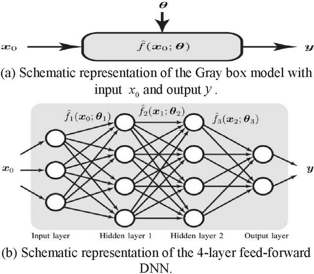
Figure 4 and a parameter vector define the Gray-box input-output model in (a). If has a complex form, such as the one seen in, it is referred to as an artificial neural network (b) [17].

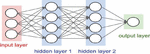
Figure 5 Schematic representation of the DNN [17].
The more advanced form of the neural network is DNN, and it consists of output, input, and input layers. Depending on the complexity of the 5G digital signal processing, hidden layers can be extended to multiple layers, whereas the input and output layers are single layers. Each layer comprises numerous nodes, and the impacts are only felt by the layers next to it. The schematic representation of the DNN is given in Figure 5. Linear and Nonlinear are two main components of the neighbouring layers. The linear component supervises each layer’s linear relationship between input and output. It has two kinds of operations: multiplication (represented by the weight ) and addition (expressed by the bias ). However, in most realistic conditions, we are confronted with nonlinear problems that cannot be solved using the linear technique. As a result, the activation function is used to handle the nonlinear component. Let and represent the output and weight matrix of the th and th layer, respectively. Let , represents the bias vector and represents the output of the th layer and it is expressed as,
| (1) |
The sigmoid and tanh function [17] approximately gives the probability distribution and they are well known activation function in DNN. The sigmoid function ranges from 0 to 1 and the tanh function ranges from 1 to 1. These activation functions give faster convergence via stochastic gradient descent (SGD). The ReLU function is another effective activation function. The ReLU function increases linearly when and it will become zero when and it is limited to [0, 1] or [1, 1]. Even after several non-linear processes, the gradient is not zero.
| (2) | |
| (3) | |
| (4) |
For the sake of simplicity, the transmission expression for multiple hidden layers can be defined in (5) as given below.
| (5) |
The sigmoid function and the softmax function are the most popular choices for the output layer. The softmax function, which can be defined as:
| (6) |
is primarily used for multiclass classification. Deep learning algorithms frequently require a large amount of data, referred to as the training set, to be fed into the system for the system to adjust itself adaptively to the best offline state. In Figure 6 schematic representation of the RNN is given and it can be readily seen that the previous data information is summarised as a state to solve the output with the current input .
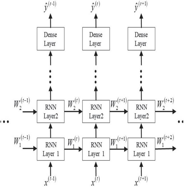
Figure 6 Schematic representation of the RNN [18, 19].
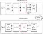
2.2 OFDM System Architecture
The block diagram of the OFDM symbol generation is given in Figure 7.
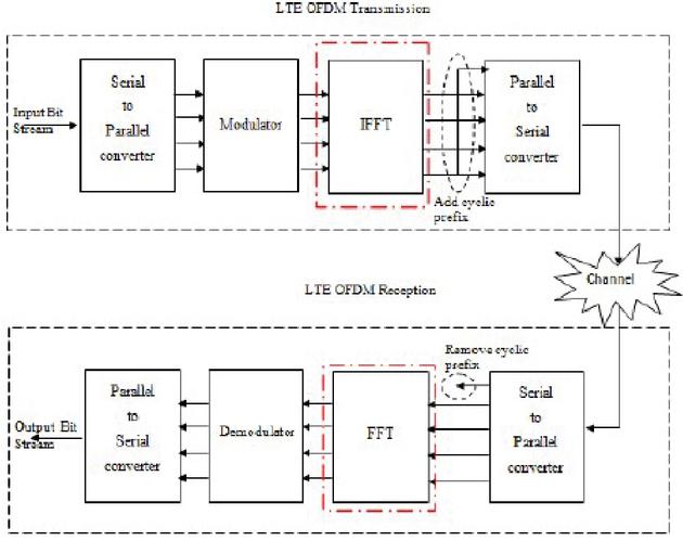
Figure 7 Block diagram of the OFDM signal transmission [20].
The complex modulated data symbols are generated through digital modulation techniques. The modulator output is converted to the parallel data stream through serial to parallel transmission procedure. The Inverse Fourier Transform (FT) technique is used for transforming the frequency domain symbols to time domain symbols. To mitigate the fading effect and to avoid the ISI, CP is inserted, and CP length is greater than the maximum value of the delay spread. The multi-tap channel is represented as,
The received signal is represented as,
| (7) |
where represents the circular convolution while and denote the transmitted signal and the additive white Gaussian noise (AWGN), respectively. After the removal of the CP, at the receiver side and performing the discrete FT, the resulting signal is expressed as,
| (8) |
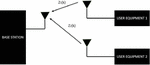
where and are the discrete Fourier transform (DFT) of and , respectively. In this work, we consider the 2 user NOMA OFDM system, and it has been assumed that the both users are transmitting their data simultaneously because they are sharing the same frequency resources. The schematic representation of the 2 user NOMA system is given in Figure 8 [21, 22]. In the case of the U/L NOMA system both the user signals at the base station (BS) will get superimposed and the resulting expression is expressed below,
| (9) |
where , and represent the AWGN channel noise, transmitted OFDM symbol, and frequency-domain received signal, respectively. The power allocated to the th user is represented as , on the th subcarrier.
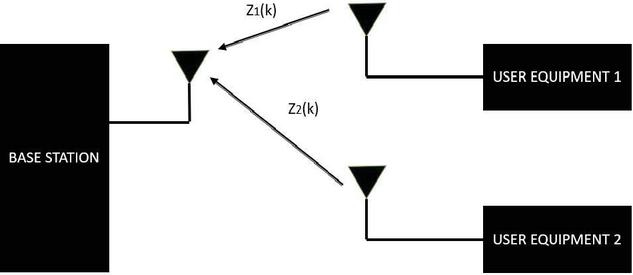
Figure 8 Two user NOMA system.
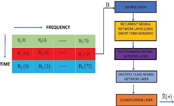
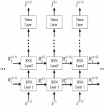
Figure 9 Schematic representation of the LSTM-based DL model.
The total transmitted power is represented by H for M number of subcarriers. The power is allocated according to the value of the power allocation factors represented as, , for th user. The total available power is limited, and the power constraint is expressed as, . Due to multipath propagation, the channel is multitap channel and the channel impulse response with complex channel gain and time delay of the th multi-path for th user is expressed as, . The DFT of the is given as . The total number of resolved paths is equal to 20 and fading links are Rayleigh distributed.
3 DL-Based NOMA Receiver
3.1 LSTM Network
The LSTM algorithm is a subset of RNN, with five layers is used. The first layer is referred to as the input layer, the second as the LSTM layer, followed by a SoftMax layer, and the final layer is referred to as the classification layer. The LSTM layer, a kind of RNN, is the fundamental component of the DNN and is commonly employed for the classification of sequence and time series data because it can leverage data time-dependence. By learning data across a sequence of phases, the LSTM algorithm will preserve data. In the LSTM algorithm-based NOMA DL detector, the OFDM subcarriers are represented as time steps. By focusing on the single time step module given by the LSTM layer, the DNN network is trained to understand multiuser detection for a specific subcarrier.
3.2 Model Training
Consider an 84 subcarrier OFDM system where the data is sent in packets. For simplicity purposes, one packet is made up of three OFDM signals. Two pilot sequences will be provided for each user, each filling up the first two OFDM symbols, while the third OFDM symbol will contain one data stream. It contains the first two OFDM symbols and the third OFDM symbol contains the single data sequence. The digital modulation method to produce OFDM data symbols is utilised for quadrature phase shift keying (QPSK), each with a two-bit/subcarrier QPSK symbol. The OFDM data packet is composed of 3-QPSK data symbols, which are randomly created with fixed pilot symbols. Inputting CP between two OFDM signals as guarding time interval, converts the frequency-domain OFDM symbol to the time-domain OFDM symbols. Three QPSK data symbols with fixed pilot symbols make up an OFDM packet, and these QPSK symbols are produced at random. By inserting the CP between two OFDM signals as the guard time interval, frequency-domain OFDM symbols are transformed to time-domain OFDM symbols. CP helps to counteract the effect of the ISI by reducing the influence of the fading channel. The channel impulse response should be less than the CP length to prevent the ISI effect. The OFDM packet is transmitted across the multipath fading connections once the CP is inserted. The BS will utilise superposition coding to combine all OFDM packets from various users, and the BS will receive all signal plus noise due to channel noise. First, a vector is created called the B function, and the incoming data packets constitute a sample of training. Feature vector B comprises the real and imaginary components of the symbols. The matrix dimension of the vector B determines the amount of features/training samples. The feature vector’s dimension is equal to the number of ODFM subcarriers number of ODFM symbols 2. The dimension of the feature vector is equal to if there are 84 subcarriers and three symbols. By assigning the matching label in the training, the DNN will be trained to discover the data symbols for the kth subcarrier. A label is a number that represents the transferred data symbols for both user’s equipment at the same time. There will be 16 combinations/labels, i.e., , since every user equipment transmits QPSK data symbols. The input vector’s dimension is determined by the real-valued vector’s length, which is 504. QPSK data is sent by all user equipment. The total number of hidden layers is 128, and the fully connected layer with an output size of 16, comes after these hidden levels because we are using DNN and there are numerous hidden layers. The classification layer will output the estimated mark, and the SoftMax layer will add a SoftMax function to its input to map all user equipment provided data symbols at the same time.
Table 1 Simulation parameters
| Number of Subcarriers | 84 | Number of training data | 500000 |
| Number of pilot subcarriers | 84 and 16 | No of deep neural network layers | 5 |
| Channel length | 20 | No of Epochs | 150 |
| Cyclic Prefix length | 20 | Learning rate | 0.02 |
| Total number of NOMA users | 2 | Batch size | 25000 |
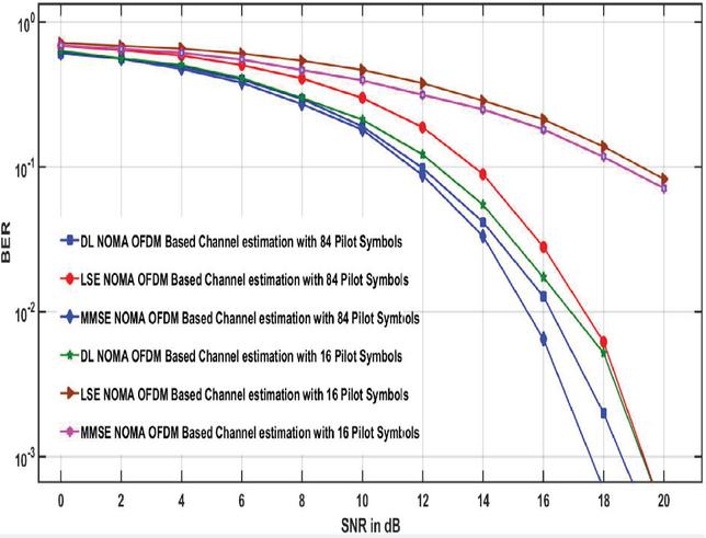
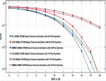
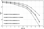
Figure 10 BER versus signal to noise ratio plots of DL NOMA detector for 84 and 16 pilot symbols.
4 Simulation Results
Simulations are carried out in this section to demonstrate the end-to-end performance of the DL methods for symbol recognition and channel estimation in the NOMA OFDM system. The simulation data will be used to train the NOMA OFDM DL detector, and the performance of the NOMA OFDM DL detector will be compared to that of standard NOMA receivers in terms of BER over a range of SNR regimes. In simulations, the DL-based solution is demonstrated to be more stable than minimal square and MMSE when fewer training pilots are employed, the CP is excluded, or there is nonlinear clipping noise. The number of subcarriers and the length of CP in our simulation are 84 and 20, respectively. The carrier frequency is set to 2.6 GHz, and there are 24 different routes. The urban channel is taken into consideration, with a maximum delay spread of 16 and QPSK complex modulates symbols.
4.1 Calculation of the Effect of Number of Pilot Numbers on the BER Performance
The DL NOMA OFDM method is compared to the MMSE and LSE approaches for signal identification and channel estimation. Because no previous data statistics of the fading channel conditions used in detection are necessary, the LSE approach delivers the lowest end-to-end system performance (see Figure 10).
The MMSE method, on the other hand, has the highest performance since the fading channel’s 2nd order data statistics are believed to be known and used for OFDM data detection. The DL based NOMA detector has good end-to-end performance than the LSE technique and is comparable to the MMSE technique.
Table 2 System parameters ReLU
| Parameter Value | Value |
| OS | Windows 10 |
| Framework | TensorFlow |
| Coding | Python 3.5 and MATLAB |
| Fading links | MIMO channel and AWGN fading channel |
| Channel Fading | Rayleigh distribution |
| Number of user devices per cluster | 2 |
| Number of antennas equipped at the transmitter | 4 |
| Number of antennas equipped at the receiver | 4 |
| Modulation Symbols | QPSK |
| Number of training samples | 409,600 |
| Total transmitted power per antenna | 2 W |
| Power allocation factor | 0.8 |
| Hidden layer | ReLU |
The maximum channel delay is 16 sampling periods and a very low number of pilot symbols are used for conduction simulations and it will give better spectral efficiency. Again, it is interesting to see the results we get by considering only 16 pilot symbols. The performance is worst as compared to the scenario when 84 pilot symbols are considered. For both 84 and 16 pilot symbols, the DNNs input and output will stay unchanged. Figure 10 reveals that while only 16 pilot symbols are used, the BER for both the minimum mean square and LSE techniques remains stable as SNR reaches 10 dB, while the DL technique also decreases its BER as SNR increases, showing that the DL NOMA detector is robust, and it is independent to the number of pilots used for the detection of the OFDM symbols. Based on the training data symbols produced from the DL model, the explanation for the superior performance of the DL-based detector is that the characteristics of the wireless fading channels can be studied.
4.2 Effect of the CP on the System Performance
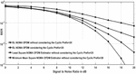
As previously mentioned, the CP is needed to transform the physical channel’s linear convolution into circular convolution and minimise ISI. Yet transmission does cost time and power. We are examining the efficiency of CP removal in this experiment. The BER curves for a DL NOMA network without CP are seen in Figure 11.
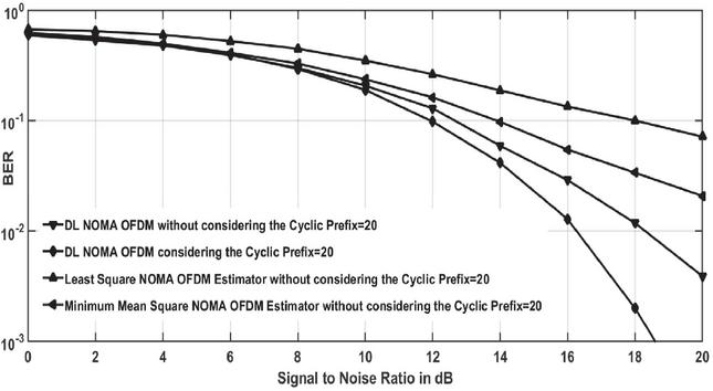
Figure 11 BER versus signal to noise ratio plots of DL NOMA detector with and without considering the CP.
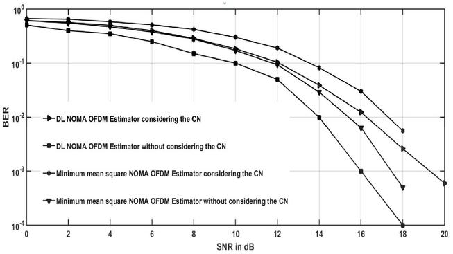
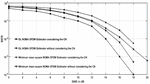
Figure 12 BER versus signal to noise ratio plots of DL NOMA detector with and without clipping noise [CN-Clipping Noise].
Neither MMSE nor LSE can provide the exact information about the fading channel coefficients. For SNR beyond 15 dB, the precision tends to be saturated. The DL methods, on the other side, continue to be successful in the estimation and detection of the channel. Again, this finding illustrates that the capabilities of the wireless fading channel have been revealed and can be mastered by the DNNs in the training stage.
4.3 Effect of the Filtering and the Clipping Distortion
One of the difficulties in the OFDM system is the peak-to-average power ratio and this difficulty is removed by using filtering and clipping. But after performing the clipping operation, we are encountering the problem of the non-linear noise, and this reduces the end-to-end system performance.
| (10) |
Where and denote the phase shift and threshold, respectively. Figure 12 demonstrates the end-to-end performance of the MMSE and DL detector when the DL NOMA network is encountered with the nonlinear noise.
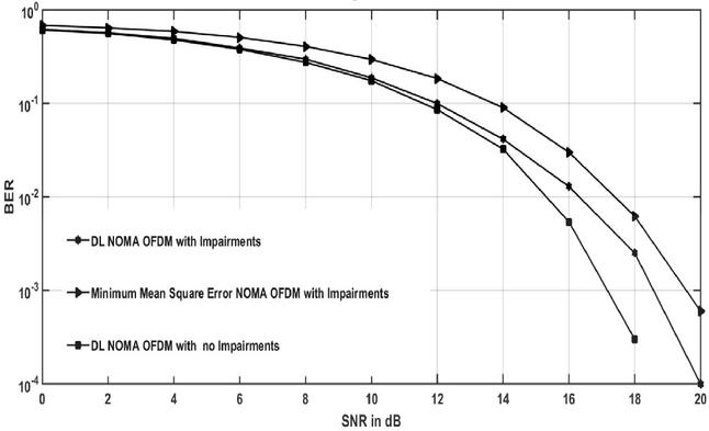
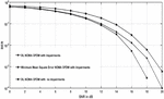
Figure 13 BER plots considering all adversities.
The simulation curves demonstrate that for clipping ratio 1, the performance of the DL based detector is very good as compared to the minimum mean square detector performance for SNR greater than the 15 dB provided that the DL technique is more robust to the clipping distortion.
Figure 13 compares minimum mean square estimation with the DL detector considering all practical conditions, excluding the CP, and clipping distortion. The curve indicates that the efficiency of the NOMA detector based on DL is higher than the traditional detectors but, as we have seen before, has a difference with detection performance under ideal circumstances.
4.4 Robustness Analysis
In the online stage, the channel coefficients are generated with similar data sets that we have in the case of the offline training. But in real time propagation conditions, there is a gap between the offline and the online deployment. It is also important that these mismatches are sufficiently stable for the trained models. The curves displayed in Figure 14 the influence of the variance in the fading relation statistics used during the preparation and deployment periods. The BER plots are seen in Figure 14 where the maximum delay spread and the number of multipath in the testing stage differ from the parameters used in the training stage. Changes in fading links data statistics do not affect major impairment to the efficiency of data symbol detection in Figure 14.
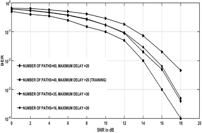
Figure 14 BER plots considering the gaps between deployment and training steps.
4.5 Impact of Learning Rate
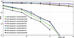
In Figure 15, the BER versus SNR in dB is plotted for both users for various values of the learning rates.
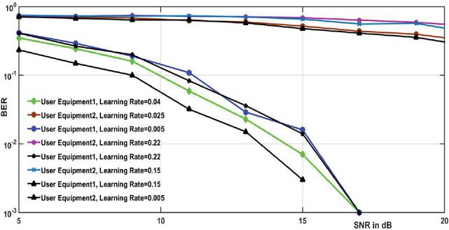
Figure 15 BER plots of DL NOMA detector for various values of the learning rates.
The curves demonstrate that the BER performance improves with lower learning rates, and it proves that a good learning rate will cause rapid updates of the weights in the DL NOMA detector, and we get very high value of the validation error. It can be readily seen that a very high accuracy can be achieved by a lower learning rate. However, the large number of iterations are required because of the very slow convergence rate. While a lower learning rate, e.g., 0.003, achieves greater precision, since more changes are needed, it leads to slow convergence. The learning threshold has been set to be 0.02 for all the other simulation cases, given a trade-off between the accuracy of the testing and the training period.
5 Conclusion
In this paper, the performance of a DL-based NOMA OFDM system is compared to that of traditional SIC NOMA methods. The simulation curves show that variation affects the channel fading data statistics utilised during the training and testing stages. The BER graphs show that the maximum distribution of delay and the number of multipath differ from the parameters used in the training stage during the testing phase. Changes in data statistics for fading connections have no significant impact on data symbol identification performance. The BER graphs show that the maximum distribution of delay and the number of multipath in the testing stage differ from the parameters utilised at the training stage. Changes in data statistics for fading connections have no significant impact on data symbol identification performance. A lower learning rate yields a lower BER, but a greater learning rate allows the DNNs weights to be altered more readily, yielding a bigger validation error. Although a lower learning rate, such as 0.003, results in better consistency, it also adds to slow consolidation when additional improvements are needed. The learning level has been set at 0.02 for all other simulation circumstances, considering the trade-off between testing precision and training duration.
References
[1] Pandya S, Wakchaure MA, Shankar R, Annam JR. “Analysis of NOMA-OFDM 5G wireless system using deep neural network”, The Journal of Defense Modeling and Simulation, March 2021. doi:10.1177/ 1548512921999108
[2] Bhardwaj L, Mishra RK, Shankar R. “Sum rate capacity of non-orthogonal multiple access scheme with optimal power allocation”, The Journal of Defense Modeling and Simulation. January 2021. doi:10. 1177/1548512920983531
[3] Chaudhary BP, Shankar R, Mishra RK. “A tutorial on cooperative non-orthogonal multiple access networks”, The Journal of Defense Modeling and Simulation. February 2021. doi:10.1177/1548512920986627
[4] Ravi Shankar, Ritesh Kumar Mishra, “An investigation of S-DF cooperative communication protocol over keyhole fading channel”, Physical Communication, vol. 29, pp. 120–140, 2018. https://doi.org/10.1016/j.phycom.2018.04.027.
[5] Shankar R. “Examination of a non-orthogonal multiple access scheme for next generation wireless networks.” The Journal of Defense Modeling and Simulation. September 2020. doi:10.1177/1548512920951277
[6] Hansika Hewamalage, Christoph Bergmeir, Kasun Bandara, “Recurrent Neural Networks for Time Series Forecasting: Current status and future directions”, International Journal of Forecasting, vol. 37, pp. 388–427, 2021. https://doi.org/10.1016/j.ijforecast.2020.06.008
[7] Dey, Prasanjit, Chandan Kumar, Mitrabarun Mitra, Richa Mishra, S. K. Chaulya, G. M. Prasad, S. K. Mandal, and G. Banerjee. “Deep convolutional neural network based secure wireless voice communication for underground mines.” Journal of Ambient Intelligence and Humanized Computing (2021): 1–20.
[8] Elwekeil M, Jiang S, Wang T, Zhang S. “Deep Convolutional Neural Networks for Link Adaptations in MIMO-OFDM Wireless Systems,” in IEEE Wireless Communications Letters, vol. 8, no. 3, pp. 665–668, June 2019, doi: 10.1109/LWC.2018.2881978.
[9] Nyländen T, Janhunen J, Silvén O, Juntti M. “A GPU implementation for two MIMO-OFDM detectors,” 2010 International Conference on Embedded Computer Systems: Architectures, Modeling and Simulation, 2010, pp. 293–300, doi: 10.1109/ICSAMOS.2010.5642054.
[10] Wang S, Yao R, Tsiftsis TA, Miridakis NI, Qi N. “Signal Detection in Uplink Time-Varying OFDM Systems Using RNN With Bidirectional LSTM,” in IEEE Wireless Communications Letters, vol. 9, no. 11, pp. 1947–1951, Nov. 2020, doi: 10.1109/LWC.2020.3009170.
[11] Kojima S, Maruta K, Ahn C. “Adaptive Modulation and Coding Using Neural Network Based SNR Estimation,” in IEEE Access, vol. 7, pp. 183545–183553, 2019, doi: 10.1109/ACCESS.2019.2946973.
[12] Chikha HB, Almadhor A, Khalid W. “Machine Learning for 5G MIMO Modulation Detection.” Sensors (Basel). 2021;21(5):1556. Published 2021 Feb. 24. doi:10.3390/s21051556
[13] Sai-Chandra-Kumari Kalla, Christian Gagné, Ming Zeng, and Leslie A. Rusch, “Recurrent neural networks achieving MLSE performance for optical channel equalization,” Opt. Express 29, 13033–13047 (2021).
[14] Zhu X, Sheng Z, Fang Y, et al. “A deep learning-aided temporal spectral ChannelNet for IEEE 802.11p-based channel estimation in vehicular communications.” J. Wireless Com. Network 2020, 94 (2020). https://doi.org/10.1186/s13638-020-01714-4
[15] Ashish IK, Mishra RK. “Performance Analysis For Wireless Non-Orthogonal Multiple Access Downlink Systems,” 2020 International Conference on Emerging Frontiers in Electrical and Electronic Technologies (ICEFEET), pp. 1–6, 2020. doi: 10.1109/ICEFEET49149.2020.9186987.
[16] Singh S, Mitra D, Baghel RK. “Analysis of NOMA for Future Cellular Communication,” 2019 3rd International Conference on Trends in Electronics and Informatics (ICOEI), pp. 389–395, 2019. doi: 10.1109/ICOEI.2019.8862527.
[17] Erpek T, O’Shea TJ, Sagduyu YE, Shi Y, Charles Clancy T. “Deep learning for wireless communications”, Development and Analysis of Deep Learning Architectures, pp. 223–266. Springer, Cham, 2020.
[18] Shoeibi, Afshin et al. “Epileptic Seizures Detection Using Deep Learning Techniques: A Review.” International Journal of Environmental Research and Public Health vol. 18,11, 5780. 27 May 2021, doi:10.3390/ijerph18115780
[19] Zappone A, Di Renzo M, Debbah M. “Wireless Networks Design in the Era of Deep Learning: Model-Based, AI-Based, or Both?,” IEEE Transactions on Communications, vol. 67, no. 10, pp. 7331–7376, Oct. 2019. doi: 10.1109/TCOMM.2019.2924010.
[20] Thota S, Kamatham Y, Paidimarry CS. “Analysis of Hybrid PAPR Reduction Methods of OFDM Signal for HPA Models in Wireless Communications,” IEEE Access, vol. 8, pp. 22780–22791, 2020, doi: 10.1109/ACCESS.2020.2970022.
[21] Khansa AA, Yin Y, Gui G, Sari H. “Power-Domain NOMA or NOMA-2000?,” 2019 25th Asia-Pacific Conference on Communications, pp. 336–341, 2019. doi: 10.1109/APCC47188.2019.9026468.
[22] Simon MK, Alouini M. “Digital Communications Over Fading Channels (M.K. Simon and M.S. Alouini; 2005) [Book Review],” IEEE Transactions on Information Theory, vol. 54, no. 7, pp. 3369–3370, July 2008. doi: 10.1109/TIT.2008.924676.
Biographies

Ravi Shankar received his BE degree in Electronics and Communication Engineering from Jiwaji University, Gwalior, India, in 2006. He received his MTech degree in Electronics and Communication Engineering from GGSIPU, New Delhi, India, in 2012. He received a PhD in Wireless Communication from the National Institute of Technology Patna, Patna, India, in 2019. He was an assistant professor at MRCE Faridabad, from 2013 to 2014, where he was engaged in researching wireless communication networks. He is presently an assistant professor at MITS Madanapalle, Madanapalle, India. His current research interests cover cooperative communication, D2D communication, IoT/M2M networks and networks protocols. He is a student member of IEEE.

T. V. Ramana is working as Professor in computer science and engineering, Chitkara University, Himachal Pradesh, India. He completed Ph. D in JNTUH, Hyderabad. His research interests include software engineering, computer system architecture, machine learning and IOT.

Preeti Singh, Assistant Professor, MSc.(Electronics), (UIET, CSJM, University, Kanpur), M.Tech. (Tezpur University), Area of Specialization: Digital Design & Technology/Antenna Design, Total experience: 8 Publications Conferences: 02.

Sandeep Gupta, Assistant Professor, Electrical Engineering Department, JECRC University, Jaipur (Rajasthan), JECRC University, Jaipur (Rajasthan).

Haider Mehraj received his B.Tech in Electronics and Communication Engineering from the Guru Nanak Dev University, Amritsar, India in 2009 and M.Tech in Communication and Information Technology from National Institute of Technology, Srinagar, India in 2011. He is currently pursuing PhD in Biometrics at the National Institute of Technology, Srinagar, India and working as Assistant Professor in BGSB University, Rajouri, India. He has a number of national and international publications to his credit. His research interests include Biometrics, Image Processing, Deep Learning, and Pattern Recognition.
Journal of Mobile Multimedia, Vol. 18_2, 451–474.
doi: 10.13052/jmm1550-4646.18214
© 2021 River Publishers