An Analysis on Polygonal Approximation Techniques for Digital Image Boundary
Kiruba Thangam Raja and Bimal Kumar Ray*
School of Information Technology and Engineering, Vellore Institute of Technology, Vellore, Tamil Nadu, India
E-mail: rkirubathangam@vit.ac.in; bimalkumarray@vit.ac.in
Corresponding Author
Received 27 April 2021; Accepted 24 June 2021; Publication 26 August 2021
Abstract
Polygonal approximation (PA) techniques have been widely applied in the field of pattern recognition, classification, shape analysis, identification, 3D reconstruction, medical imaging, digital cartography, and geographical information system. In this paper, we focus on some of the key techniques used in implementing the PA algorithms. The PA can be broadly divided into three main category, dominant point detection, threshold error method with minimum number of break points and break points approximation by error minimization. Of the above three methods, there has been always a tradeoff between the three classes and optimality, specifically the optimal algorithm works in a computation intensive way with a complexity ranges from O (N) to O (N).The heuristic methods approximate the curve in a speedy way, however they lack in the optimality but have linear time complexity. Here a comprehensive review on major PA techniques for digital planar curve approximation is presented.
Keywords: Contour, break points, split and merge, dominant points, polygonal approximation, digital planar curve, integral square error, chain code, digital image boundary.
1 Introduction
The computationally resource intensive activity such as storing, processing and visualizing large and noisy object have been a challenge for many decades. Representing the high density image in the form of 2D contour shape reduces time and space in object recognition. Shape is a significant inherent property of any object. Here the contour lines along with points acts as an object identification criteria and its points are expressed as, {x(n), y(n)}, n 0, 1, 2, 3,…, N 1, where N is the total number of contour points. Consequently the total number of points can still be reduced without distorting the original shape by approximating the digital curves using polygonal approximation (PA). People identify objects based on their shape due to the fact that it has been used or seen in their day to day life. However when it comes to the machine recognition of the shape the image plays a critical role on how it is presented to the system in 2D or 3D images. Aside for quick identification, 2D images are very important as it can be easily recognized based on the outline of the objects. Hence shape recognition is the foremost feature of any object identification. One of the key steps in image analysis is the approximating digital curves using polygon. PA is also utilized in contour feature extraction and segmentation that can be applied in object detection and recognition. It reduces the resources and represents the image objects in a much robust manner. Digital images play a critical role in relatively all areas of engineering and sciences. Specifically, in the field of object recognition, multimedia, machine vision, shape representation, vector data compression, digital cartography and classification.
Polygonal approximation is a classic problem in the field of pattern recognition and digital image processing. Attneave [4] pioneered the idea that object contour information is concentrated at the corners or at high curvature points of that object. Much of the effort and several techniques have been produced to cover this area of research since then. However, these approximation techniques have varied accuracy and time complexity. The major objective of this field of work is to find better and novel solutions to represent, store and recognize the image data without compromising on the object shape information. The effectiveness of extracting the distinctive features from the digital image pattern is the key starting point in object simplification. The major features of a contour image include vertices, edges and boundaries. Vertices or corners are the significant points where two relatively straight line segments intersect. Finding the corners points is the first step in any approximation technique. Next, the dominant corners points are detected and thereby subsequently reducing the less-significant corners. Finally, the dominant points alone are joined and the objects are approximated with some error values. The prime criteria of PA include faster execution with near to the minimal memory usage.
PA algorithms are extremely useful in wide range of applications because of its compactness and its insensitiveness towards noise. These features of PA made it to have many applications which includes understanding shapes [4], digital cartography [12] biological signal processing [44], image matching [19] image analysis [28] path planning with curvilinear obstacles [20].
In this paper, a comparison of different techniques for PA is presented. Section 2 describes the problem and Section 3 gives the importance of freeman chain code in gathering the breakpoints of a digital planar curve. Section 4 comprises of the detailed classification of different PA techniques which has the Subsections 4.1, 4.2 and 4.3. The Subsection 4.1, 4.2 and 4.3 present the brief review of heuristic algorithms, metaheuristic algorithms and optimal algorithms. Section 5 narrates the standard measures useful in comparing the efficiency of the different PA algorithms. Section 6 concludes the paper.
2 Problem Definition
The problem of PA may be formulated by an ordered collection of points that indicates a digital curve, C with ‘ n ‘curve points. It is denoted by C {p, p…p}.
The aim of PA is to detect the subset of points in the curve as S {s, s,…,s}, where m n, m denotes the number of points in S whereas n denotes the number of curve points in the digital curve, C which means the curve S is a subset of the curve C. Here, the m points are arranged in clockwise/counter clockwise direction that configures a set of m line segments which preserves the key features of curve C. These set of points constitute the line segments so that the polygon thus constructed describes the native shape with minimal distortion. The accuracy of approximation is given by the error values. In the literature, Masood [25, 26] handles the PA problem by removing the initial point of redundant points in a digital curve using Freeman chain code.
Breakpoint of a digital curve is a point on its image boundary where the curve takes turn at the point. Alternatively, A point on a curve is considered to be a breakpoint when the chain code [15] (Figure 1) of two consecutive points differ. The breakpoints which are prominent points determine the shape of a curve. In further processing some of the breakpoints can be eliminated using some criterion and the resultant set of breakpoints are called dominant points or significant points which are the prime factors in determining the shape of an object.
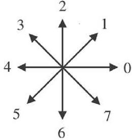
Figure 1 Eight directional Freeman chain code.
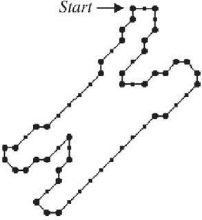
Figure 2a A closed digital curve exhibiting the shape of a chromosome indicating the dominant points.
In general, all the breakpoints are considered as the candidates points for vertices of a polygon approximating a digital curve. For approximating a digital curve, some of the breakpoints are considered to be redundant break points based on the noisy nature due to digitization of the original contour. Such redundant breakpoints may be discarded preserving the most prominent breakpoints on performing the polygonal approximation. By performing the PA, the computation time in applications such as computer vision can be drastically reduced by the collection of candidate breakpoints and by discarding the redundant breakpoints focusing only on the most prominent breakpoints. Different techniques are used in discarding the less significant or redundant breakpoints.
The Figure 2a shows the closed digital curve forming the shape of a chromosome and is approximated by subsets of line segments which are formed by m consecutive breakpoints {p, p…p} indicated with solid circle.
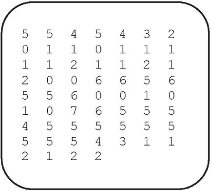
Figure 2b Chain code for chromosome.
3 Freeman Chain Code
The chain code (Figure 1) identifies the breakpoints from the digital planar curve by joining series of straight line segments of specified length and direction. Assuming the total number of contour points as n, and the array CC where CC (n) 0,1,2,3…7 which contains the chain code of the contour. It assigns an integer value CC ranging from 0 to 7 to each curve point p based on the direction of the consecutive point. The Figure 1 illustrates the chain code value based on Freeman’s method for all the possible directions [15].
Among the curve points of the digital curve, only the break points are selected which identifies boundary turn. It means that the chain code of two consecutive points CC and CC differ. The highlight of this algorithm is that it produces absolutely zero approximation error. After using the chain code as given in Figure 1, the identified set of break points for the chromosome shape can be seen in Figure 2a. The Figure 2b gives the chain code generated for the chromosome shape of Figure 2a. From Figure 2b we can understand how the chain code can be generated based on Freeman’s method.
4 Classification of Polygonal Approximation Algorithms
The various approximation methods can be classified as heuristic, metaheuristic, and optimal algorithms [1]. The Figure 3 represents a variety of contours that is approximated using some PA algorithm. Figure 3 gives the examples of contours like apple, semicircle shaped curve, leaf shaped curve and chromosome shaped curve after approximated using PA algorithms. Many researchers have tested PA algorithms on various contours in MPEG dataset [53].
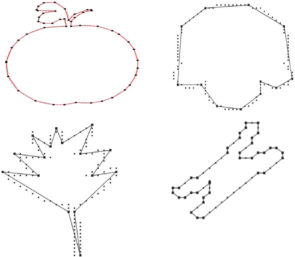
Figure 3 Illustrations of polygonal approximations on various contours.
4.1 Heuristic Algorithms
Non-optimal polygonal approximations can be produced by heuristic algorithms. The computational costs of heuristic algorithms are comparatively low compared to other algorithms.
Heuristic algorithms generally follow a greedy approach which may be further categorized into the following approaches namely: sequential scan approach [35], split approach [12, 33, 43] merge approach [15, 24–26] [and split-and-merge approach [17, 29, 34, 48].
Classical methods were developed to solve the PA problem during the 1970s, when Ramer [33] proposed a split-based approach that seeks a PA of the digital curve by an iterative technique with minimum number of vertices, based on a single preset error constraint. However, the limitation with this algorithm is that the final outcome is related to the initial solution, which means even an insignificant vertex that does not corresponds to an expected vertex may be mistakenly included in the final solution.
Ramer’s work has been further carried on which uses the split-and-merge approach [29]. It utilizes the vertical distance as the criterion function. In this, the initial segmentation is performed randomly and the approximation is based on initial line segments of the boundary points with least square error. Finally, the split- and- merge occurs for large and small segments respectively. Hence this becomes a scale dependent and may miss some key vertices and it is less sensitive to orientation. Gaussian smoothing is used to discover the cardinal curvature points that ultimately influences the time complexity [3]. A very recent algorithm [14] based on the modification of the Ramer, Douglas–Peucker method [12] is a split based scale-independent algorithm. It subdivides a digital curve into its most perceptually important straight line segments. This method overcomes the general drawbacks of RDP method wherein it is influenced by the preset error with the avoidance of contour symmetry.
Duda and Hart [13] method is a threshold based splitting method that starts by finding the initial and terminal point of the line segment, next it searches for the greatest departure point from the straight line by joining both ends. Then the departure point which is considered as an anchor point for the line segment is compared to that threshold value. These steps are iterated such that the data points are well fitted by the line segments. The adjacent break-points are joined to obtain the polygon. However this technique requires multiple passes through the data. Ray and Ray [34] split-and-merge technique is insensitive to scales and orientations, which has no effect on the curve. Due to its simplicity, it is found that the time complexity is less than the algorithm proposed by Ansari and Delp [3]. Above all, this technique is more reliable even in the presence of noise.
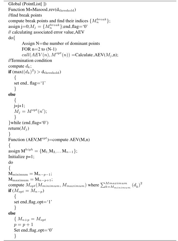
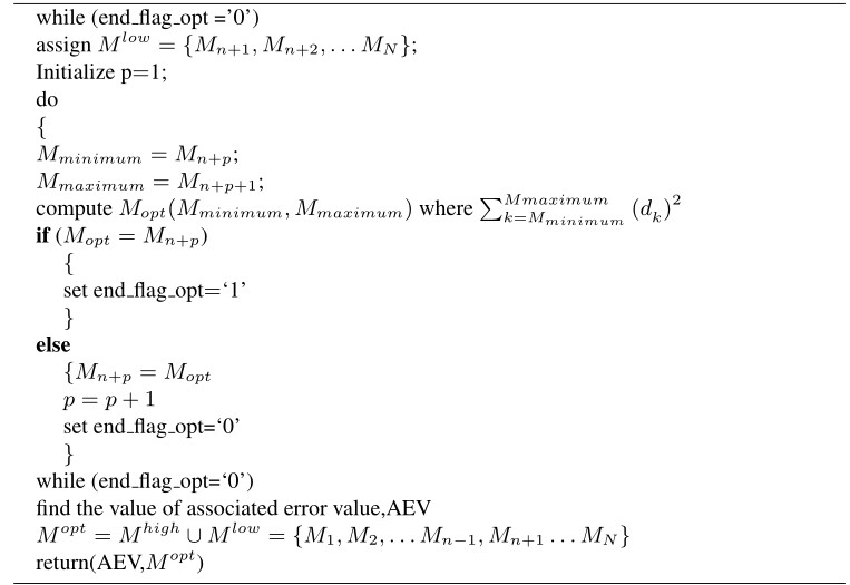
Masood’s method [26] starts with the grouping of the breakpoints with the least number of line segments such that every pixel of the digital curve on the line segment is viewed to be the starting set of dominant points. At that point, the algorithm continues recursively with suppressing each one of the break point at a time so that deleting the point will have only a minimum effect in its immediate neighborhood as well as optimizing the areas of the dominant points for least precision score. This method implies reliability and thus improves the global fit for optimization and known for precision however reliability is questionable as it is sensitive to digitalization [26]. Since this method starts with the maximum possible group of dominant points. The dominant points are deleted based on a termination criterion. Similar to Masood’s method, Carmona’s technique [8] also starts with the sequence of break points with the initial set of dominant points. It further iteratively removes the dominant points which have the least influence on the global fit of the line segments. The major focus is on the reliability than on precision in comparison to Masood’s method. It is very clear from the results that this method has a tendency to be relaxed in the maximum allowable variation for the whole curve. The comparison values of the results are shown in Tables 1 and 2 for some of the above approach which are mentioned here along with their pseudo code,
Algorithm 1 Pseudocode of RDP algorithm
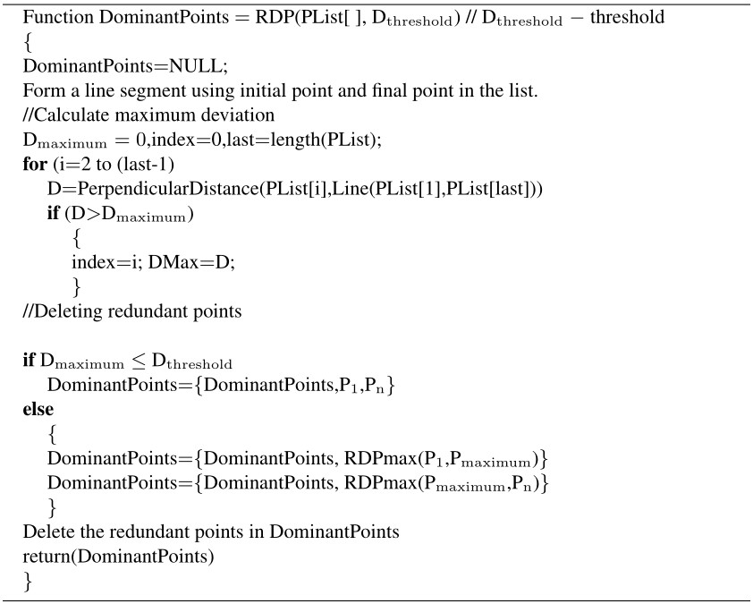
All the selected non-parametric dominant point detection methods presented since RDP algorithm deployment and a number of modification effected on to the RDP are presented. Here the recent methods are compared with RDP algorithm result based on the values obtained for different shapes. In the RDP algorithm, initially a line segment is formed using the initial and final point in the list, then the maximum deviation is calculated. Next the redundant points are deleted based on certain criteria.
Algorithm 2 Pseudocode of Masood’s reverse polygonization’s method
Carmona et al.’s [7] approach is a very simple approach for approximating polygon. In this method’s suppression of breakpoints are used to compute the dominant points and in turn approximate the polygon.
Algorithm 3 Pseudocode of Carmona’s break point suppression method
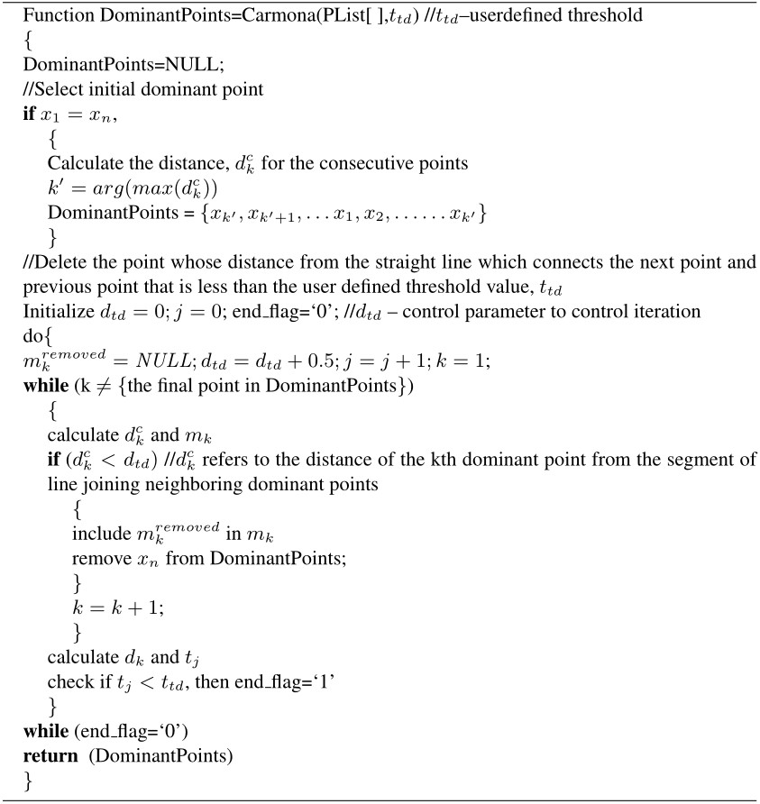
Table 1 indicates the critical parameters to assess the different algorithms. Starting from the number of dominant points, here the Figure of Merit, FOM (defined by the ratio of compression ratio to integral square error) and CR values is high when they have large values in contrast to the maximum deviation, max (d) and Integral Square Error, ISE, which has to be less in values [36] Section 5 describes about the various parameters such as ISE,FOM ,CR and their significance in evaluating the different PA algorithms.
Table 1 Comparative analysis of different algorithms for various shapes
| Number | Number | max | |||||
| of | of | ||||||
| Pixels | Dominant | ||||||
| Shape | Method | (m) | Points (n) | (d) | ISE | FOM | CR |
| Maple Leaf | RDP | 424 | 35 | 1.98 | 202.3 | 0.06 | 12.11 |
| Masood | 424 | 50 | 1.23 | 46.34 | 0.18 | 8.48 | |
| Carmona et al. | 424 | 20 | 4.06 | 847.89 | 0.03 | 21.2 | |
| Hammer | RDP | 388 | 13 | 1.65 | 92.94 | 0.32 | 29.85 |
| Masood | 388 | 15 | 1.46 | 38.35 | 0.67 | 25.87 | |
| Carmona et al. | 388 | 10 | 2.32 | 177.4 | 0.22 | 38.8 | |
| Africa | RDP | 291 | 25 | 1.81 | 102.93 | 0.11 | 11.64 |
| Masood | 291 | 35 | 1.21 | 31.26 | 0.27 | 8.31 | |
| Carmona et al. | 291 | 14 | 3.81 | 547.22 | 0.04 | 20.79 | |
| Tin_opener | RDP | 278 | 24 | 1.83 | 127.99 | 0.09 | 11.58 |
| Masood | 278 | 34 | 1.4 | 40.37 | 0.2 | 8.18 | |
| Carmona et al. | 278 | 22 | 2.28 | 214.6 | 0.06 | 12.64 | |
| Dog | RDP | 343 | 36 | 2 | 149.19 | 0.06 | 9.53 |
| Masood | 343 | 49 | 1.26 | 43.19 | 0.16 | 7.00 | |
| Carmona et al. | 343 | 54 | 1.39 | 54.26 | 0.12 | 6.35 |
In Table 1, the max (d) score range is less for Masood’s [25] method as compared to the RDP [12, 33] and Carmona et al. algorithm [8]. A similar range is followed for ISE values also. The range variation is maintained in the same order as above for FOM and CR as well.
The following Table 1 and Figure 4 shows the important PA approximation methods [11] for different shapes such as maple leaf, hammer, Africa, tin opener and dog. The table 1 describes the number of dominant points( n), number of pixels (m), maximum deviation (max(d)), ISE, FOM and CR for various shapes based on important approximation methods. For example, for the maple leaf shaped curve of 424 pixels, when we apply the RDP [12, 33] algorithm we get a maple leaf curve approximated with 35 dominant points where the maximum deviation is found to be 1.98 with an integral square error of 202.3 having 0.06 of FOM and CR as 12.11. Again Masood’s [25] technique when applied on the same maple leaf shaped curve gave a approximated curve with 50 dominant points where the maximum deviation is found to be 1.23 with 46.34 as ISE. The FOM and CR is found to be 0.18 and 8.48. Similarly when the Carmona et al. algorithm [8] is applied we receive an approximated curve with 20 dominant points with the maximum deviation as 4.06 and the ISE is found to be 847.89. The FOM and CR is found to be 0.03 and 21.2 respectively.
Figure 4 shows the results of the maple leaf shaped curve. Similarly the comparative analysis and results for other shapes for these three algorithms can be understood from Table 1 and Figure 4.
In the Carmona et al. [7] approach at first, the break points us computed where the boundary makes a turn is computed. If a breakpoint is found to be redundant, then it is deleted, when it is found to be quasi-collinear points with the predecessive and successive break points. To delete the redundant points, a threshold distance is set and the threshold is increased until the deletion criterion is satisfied. Based on the requirement of the end user, the threshold value may be selected. The threshold value of 0.5 is considered for exact contours with maximum dominant points. To attain less precise contours with less dominant points, 0.7 is considered to be the threshold value.
The Table 2 shows the comparative results of Masood and Haq [24] with Carmona et al. [8], which are similar in computational complexity. The measure FOM2 is defined as the ratio between (CR) and ISE. Rosin [36] proved that both the terms in the FOM such as compression ratio and integral square error are unbalanced making the FOM measure to be biased towards approximations for lower ISE values.
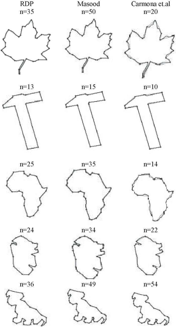
Figure 4 Results of different shapes for significant approaches.
Table 2 comparative results of Masood and Haq [24] with Carmona et al. [8]
| r, Carmona et al. | , Carmona et al. | Masood et al. | |||||||||||||||||
| Contour | N | n | E | CR | ISE | FOM | FOM2 | n | E | CR | ISE | FOM | FOM2 | n | E | CR | ISE | FOM | FOM2 |
| Tin_opener | 580 | 25 | 3.4 | 23.2 | 620.1 | 0.037 | 0.868 | 20 | 5 | 29 | 1857.5 | 0.002 | 0.453 | 119 | 1 | 4.9 | 22 | 0.22 | 1.07 |
| Plane | 1015 | 20 | 6.3 | 50.8 | 6401.5 | 0.008 | 0.402 | 17 | 6.4 | 60 | 6773.8 | 0.009 | 0.526 | 258 | 1 | 3.9 | 47 | 0.08 | 0.33 |
| Rabbit | 745 | 28 | 3.6 | 26.6 | 1094.5 | 0.024 | 0.647 | 10 | 13.3 | 75 | 18253 | 0.004 | 0.304 | 102 | 1 | 7.3 | 57 | 0.13 | 0.94 |
| Screwdriver | 1677 | 8 | 9.3 | 209.6 | 25570.9 | 0.008 | 1.718 | 4 | 30.6 | 419 | 415271 | 0.001 | 0.423 | 702 | 1 | 2.4 | 142 | 0.02 | 0.04 |
| Dinosaur | 795 | 38 | 1.7 | 20.9 | 287.3 | 0.073 | 1.523 | 23 | 5.9 | 35 | 3800.8 | 0.009 | 0.314 | 155 | 1 | 5.1 | 27 | 0.19 | 0.98 |
| Hand | 1041 | 20 | 6.3 | 52.1 | 5804.1 | 0.009 | 0.467 | 15 | 16.6 | 69 | 20707 | 0.003 | 0.233 | 175 | 1 | 5.9 | 57 | 0.11 | 0.62 |
| Hammer | 2701 | 10 | 13 | 270.1 | 17346.5 | 0.016 | 4.206 | 10 | 13.2 | 270 | 17347 | 0.016 | 4.206 | 635 | 1 | 4.3 | 177 | 0.02 | 0.1 |
| sword fish | 1912 | 46 | 14 | 41.6 | 18123.8 | 0.002 | 0.095 | 22 | 13.6 | 87 | 47090 | 0.002 | 0.16 | 989 | 1 | 1.9 | 121 | 0.02 | 0.03 |
| Turtle | 553 | 29 | 2.5 | 19.1 | 235.2 | 0.081 | 1.546 | 23 | 3.9 | 24 | 707.3 | 0.034 | 0.817 | 59 | 1 | 9.4 | 54 | 0.17 | 1.63 |
| Averages | 25 | 6.6 | 79.3 | 8387.1 | 0.028 | 1.274 | 16 | 12.1 | 119 | 59090 | 0.008 | 0.826 | 355 | 1 | 5 | 78 | 0.11 | 0.64 | |
In Table 2, the results for various shapes of the two different algorithms has been given. The first column of the table lists the different contour shapes considered and each row of the table corresponds to their relative values n, E, CR, ISE, FOM and FOM2.
Carmona et al. [7] demonstrated that the measure of FOM2 gives a better performance than the measure of FOM. In Carmona et al. [8] the E values are greater than the Masood and Haq [24] The Masood’s technique [24], results in approximations with larger number of dominant points because of the low ISE values. For the threshold value, r, the FOM2 obtained by Carmona et al. is better than Masood. In most of the cases, for the threshold value, r the FOM values of Carmona et al. were a notch less than Masood’s algorithm. So with r, the Carmona et al. approach gives a slightly better FOM2 measure than Masood’s approach.
4.2 Metaheuristic Algorithms
Metaheuristic algorithms are approaches that work on stochastic optimization methods. A metaheuristic algorithm does not guarantee an optimal solution, but it is capable of providing a good solution which is very closer to the optimal results. Researchers have been applying nature inspire algorithms to solve pattern recognition and image processing problem.
Metaheuristic algorithms include genetic algorithms [18, 46], tabu search [49, 50] ant colony optimization [51], particle swarm optimization [47]. These methods have been successfully applied for the PA optimization problem. Ranking selection (RSM) was formulated for the PA of digital curves for split-and-merge method. The RSM in genetic algorithm substantially reduce the sensitivity of the traditional split-and-merge method to the initialization solution.
Nature inspired algorithm [46] have been adopted increasingly to solve the PA problem in recent years. The Meta heuristic algorithms utilized in PA with the results are shown as tabular representation. The Tables 4 and 5 shows the comparative analysis of various meta heuristic algorithms like bPSO [52], mPSO [45], GA [45] and iPSO for sample inputs. The Integer Particle Swarm Optimization, iPSO [46] uses integer coding to provide a direct solution representation as compared to other PSO. IPSO has been shown to excellent results in terms of quality and computational speed. It has produced better results compared to the Ant Colony Search method [51] and GA-based method [46, 49].
Compared to the binary version of particle swarm optimization (bPSO), the Integer Particle Swarm Optimization, iPSO [47] which uses the integer coding gives a promising performance. Based on computational efficiency, the iPSO results exhibit high performance for various shapes compared to bPSO based approaches and the mPSO is also the binary version of PSO and which is applied by a mutation operator.
The Figure 5 and Table 3 show the comparative results which highlights that iPSO is superior to other approaches. The result in table shows the best performances for the various methods on the different shapes.
The Figure 5 give the number of vertices and their ISE after approximation of the leaf shape and semicircle shaped curve for bPSO, mPSO, ga, iPSO algorithms.
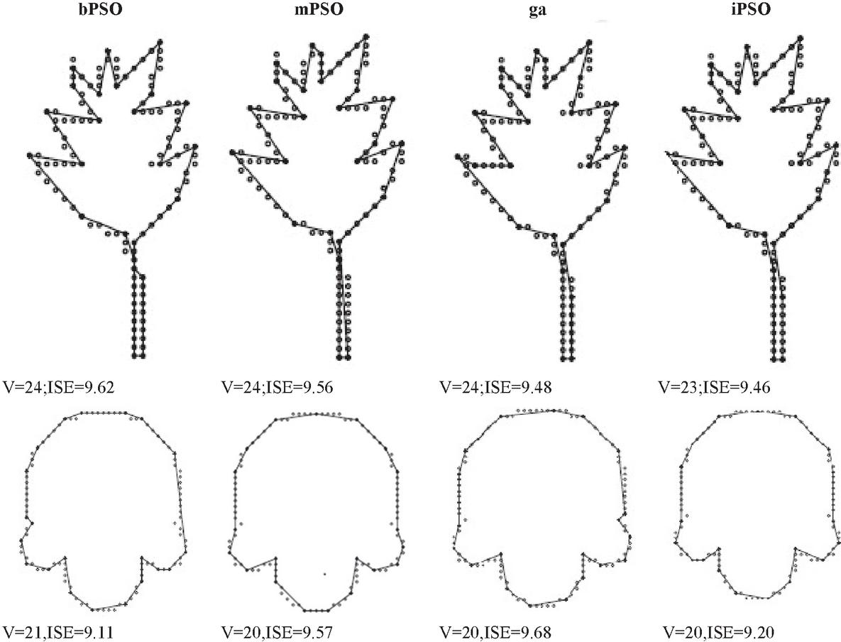
Figure 5 The sample input of leaf shape and semicircle shaped curve using meta heuristic algorithms like bPSO [52], mPSO [45], GA [46] and iPSO [47].
Table 3 The error tolerance (), number of vertices in the polygon (V), ISE, fidelity and merit between various meta heuristic algorithms like bPSO [52] mPSO [45], GA [46] and iPSO [47] for semicircle & leaf shapes
| Error | No. of Vertices | ||||||
| Tolerance, | in Polygon, | ||||||
| Shape | Method | V | ISE | Fidelity | Efficiency | Merit | |
| Semicircle | bPSO | 10 | 21 | 9.11 | 87.6 | 94.8 | 91.1 |
| mPSO | 20 | 9.57 | 94.1 | 97.3 | 95.7 | ||
| GA | 20 | 9.68 | 93.1 | 96.7 | 94.9 | ||
| iPSO | 20 | 9.2 | 97.9 | 99.1 | 98.5 | ||
| bPSO | 60 | 10 | 50.45 | 77.1 | 95.1 | 85.7 | |
| mPSO | 10 | 47.51 | 81.9 | 96.4 | 88.9 | ||
| GA | 10 | 45.39 | 87.8 | 97.3 | 91.3 | ||
| iPSO | 10 | 38.92 | 100 | 100 | 100 | ||
| bPSO | 150 | 7 | 112.25 | 82.9 | 94.2 | 88.4 | |
| mPSO | 7 | 104.23 | 89.3 | 96.6 | 92.9 | ||
| GA | 6 | 145.52 | 96.5 | 99.4 | 97.9 | ||
| iPSO | 6 | 141.29 | 99.4 | 99.9 | 99.7 | ||
| Leaf | bPSO | 10 | 24 | 9.62 | 89.8 | 95.3 | 92.5 |
| mPSO | 24 | 9.56 | 90.3 | 95.5 | 92.9 | ||
| GA | 24 | 9.48 | 91.2 | 95.8 | 93.5 | ||
| iPSO | 23 | 9.46 | 100 | 100 | 100 | ||
| bPSO | 60 | 13 | 57.65 | 83.4 | 93.8 | 88.4 | |
| mPSO | 13 | 59.7 | 80.5 | 92.5 | 86.3 | ||
| GA | 13 | 54.8 | 87.8 | 95.7 | 91.6 | ||
| iPSO | 12 | 59.94 | 100 | 100 | 100 | ||
| bPSO | 150 | 10 | 142.08 | 73.6 | 85.2 | 79.2 | |
| mPSO | 10 | 147.22 | 71 | 82.3 | 76.5 | ||
| GA | 9 | 149.09 | 89.5 | 90.3 | 89.9 | ||
| iPSO | 9 | 135.47 | 98.5 | 98.7 | 98.6 |
The error tolerance, the number of vertices after approximation, the ISE, fidelity, efficiency and Merit values of the PA algorithms such as bPSO, mPSO, ga, iPSO algorithms for the semicircle shaped curve and the leaf shaped curve can be understood from the Table 3.
Shu-Chien Huang [41] proposed a new PA algorithm based on artificial bee colony algorithm. Artificial bee colony algorithm simulates the behavior of the honey bees. There are three different groups of bees namely employed bees, onlooker bees, and scout bees. In this algorithm, the first partition of the colony holds the employed bees and the other partition holds the onlooker bees. Employed bees are related to food resource whereas the onlooker bee guides the waiting bees to receive the news about the food source. Scout bees are employed bees whose food are exhausted by the onlooker and employed bees. The scout bee do random search to find new food sources. This concept is helpful in approximating the polygonal curve. Thus polygonal approximation using an artificial bee colony algorithm uses the fitness of the associated solution. If the solution can be expressed as an “k”-dimensional vector where k refers to the number of optimization parameter as well as the number of breakpoints in a polygonal curve.
4.3 Optimal Algorithms
Optimal algorithms are also applied on to the polygonal approximations problems. The problem of determining optimal, in contrast to suboptimal, PA of digital curves can be broadly classified into two distinct optimization problems. The objective of the optimization problem is to compute the subset of segments by another polygonal curve. Optimal algorithms can be classified into two types namely, min – problem and min – # problem.
(i) min – problem: Given the native polygon curve with number of vertices, the objective is to discover the least number of vertices so that the approximation error (distortion) is minimized and this problem is called min – problem and is also known as minimum-distortion problem.
(ii) min – # problem: Given the native polygon curve with number of vertices, the aim is to compute the minimum set of vertices with predefined error such that the distance of the polygon from the contour is less than the preset error value and this problem is known as min – #.
Until recently several methods have been employed to tackle the above formulated PA problem. In this review, we explore a few of the major techniques involved in solving or nearing optimal solutions.
The main disadvantage of these types of algorithms is their high computational cost compared to other algorithms. In general, optimal algorithms work by employing dynamic Programming [6, 29, 30] or A*-search approach [38, 39] uses dynamic programming and basically limits to the investigative parts of the solution, quickly finding how the solution of the comparison for the purpose of subdivision can be reduced. He also indicated the extension of his work to polynomial fittings of known functions. Gluss [16] extended Bellman’s work by implementing Stone’s [43] equation in deducing it to identify the subdivision in the line segments of a polygon, which act as a continuous non-linear function that involves two variables. Stone’s equation produce discontinuous approximation, sometimes the line segments may be broken if it not meeting at the end point of subdivision. Gluss overcomes this by adding a unique criterion function which involves derivative of known function and the line segment’s slope.
Gluss introduced a revised form of the Bellman’s algorithm to calculate the error during the computation of shortest path [16] This measurement enables one to choose the vertices which relates to a high transitivity region of the graph.
An approach based on concavity tree was initially proposed to find out the minimal length polygons and in refining the breakpoints [42]. An extended version of this concavity tree was proposed in which convex hull is used. In this approach, the concave and convex regions of the contour are indicated by the convex hulls. The distinct points relating to the convex and concave regions of the contour are prominent dominant points since they are breakpoints. Based on this approach, lesser number of dominant points is added when the contour is straight in nature and more dominant points are added for curved contours. Convex hull is the smallest polygon which holds all the required points which determines the contour’s shape.
A recent proposal [2] states the PA problem as an optimization problem using Mixed Integer Programming (MIP). A MIP involves an objective function that need to be minimized or maximized subject to a collection of linear constraints. This method does not need an initial point for PA and the computational load or time complexity is very less than other methods that have its merits. A novel graph-based approach [5] proposed to calculate the polygonal approximation. Given a closed curve, the approach creates a graph where each vertex relates to a point in this curve.
Table 4 shows the comparative analysis of important algorithms showing the number of points (N), ISE and the confirmation of optimality. Perez-Vidal [30] use the starting point of the curve as initial point and this approximation is indicated by Perez-Vidal, and trying all the points as initial point, indicated by Perez-Vidal, Salotti used the initial point of the curve as initial node, indicated by Salotti, and trying all the points indicated by Salotti [38]. Masood’s [26] method works on by selecting an initial set of points and in every iteration, one point is deleted based on the associated error of that particular point. After deletion of the point, he uses an optimization method to locate the optimal locations of the remaining points which minimizes the distortion. But this optimization process doesn’t guarantee an optimal solution.
Table 4 Comparative analyses of existing algorithms between Perez-Vidal [30], Salotti [38] and Aguilera et al. [2] to highlight the optimality of the solutions for different number of point, N
| Contour | Method | N | ISE | Optimal |
| Chromosome | Perez-Vidal | 12 | 6.06 | No |
| Perez-Vidal | 12 | 5.82 | Yes | |
| Salotti | 12 | 6.06 | No | |
| Salotti | 12 | 5.82 | Yes | |
| Masood | 12 | 5.82 | Yes | |
| Aguilera et al. | 12 | 5.82 | Yes | |
| Perez-Vidal | 15 | 3.97 | No | |
| Perez-Vidal | 15 | 3.79 | Yes | |
| Salotti | 15 | 3.97 | No | |
| Salotti | 15 | 3.79 | Yes | |
| Masood | 15 | 3.88 | No | |
| Carmona et al. | 15 | 4.27 | No | |
| Aguilera et al. | 15 | 3.79 | Yes | |
| Semicircle | Perez-Vidal | 15 | 14.4 | Yes |
| Perez-Vidal | 15 | 14.4 | Yes | |
| Salotti | 15 | 14.4 | Yes | |
| Salotti | 15 | 14.4 | Yes | |
| Masood | 15 | 14.4 | Yes | |
| Aguilera et al. | 15 | 14.4 | Yes | |
| Perez-Vidal | 25 | 4.75 | No | |
| Perez-Vidal | 25 | 4.62 | Yes | |
| Salotti | 25 | 4.75 | No | |
| Salotti | 25 | 4.62 | Yes | |
| Masood | 25 | 4.75 | No | |
| Aguilera et al. | 25 | 4.62 | Yes | |
| Carmona et al. | 26 | 4.91 | No | |
| Aguilera et al. | 26 | 4.0543 | Yes | |
| Leaf | Perez-Vidal | 13 | 55.88 | No |
| Perez-Vidal | 13 | 38.32 | Yes | |
| Salotti | 13 | 55.88 | No | |
| Salotti | 13 | 38.32 | Yes | |
| Masood | 13 | 64.85 | No | |
| Aguilera et al. | 13 | 38.32 | Yes | |
| Carmona et al. | 23 | 10.68 | No | |
| Aguilera et al. | 23 | 7.4661 | Yes | |
| Perez-Vidal | 32 | 4.45 | No | |
| Perez-Vidal | 32 | 3.45 | Yes | |
| Salotti | 32 | 4.45 | No | |
| Salotti | 32 | 3.45 | Yes | |
| Masood | 32 | 4.45 | No | |
| Aguilera et al. | 32 | 3.45 | Yes |
Carmona et al.’s [8] approach detects a sequence of dominant points on the boundaries of the contour to acquire a polygonal approximation of the shape from the original break points of the initial boundary of the contour, where the integral square is found to be zero. The breakpoints are deleted when the perpendicular distance to an approximating straight line is found to be less than the threshold value. By this approach, the redundant breakpoints are suppressed until the expected approximation is reached. The demerit of this approach is high computational complexity. Based on the results in Table 4, Perez-Vidal [30], Salotti [38] and the MIP method of Aguilera et al. [2] obtain the optimal solution.
Table 5 shows that the computation time taken by various optimal approximation methods. The demerit of Perez-Vidal [30] is the high computational time when there is increase in the number of points (N) of PA. Aguilera et al.’s [2] MIP method shows no changes with increase in number of points (N) of the PA. Salotti [38] use A* search algorithm to perform searching in a graph which is made up of the points of the curve. Based on the Salotti’s experiment the initial point of the curve is considered to be the root node. In this experiment, all points are considered as initial node to fetch the optimal solution. The analysis shows that the MIP algorithm is six times faster than the Salotti’s mechanism. The MIP method by Aguilera et al. [2] provides an optimal solution with less computation time compared to other existing dynamic programing methods [30, 39] for different number of segments (N) ranging from 10 to 50.
Table 5 Computation time between some of the available dynamic algorithm methods [2] in seconds
| Contour | Method | N 10 | N 20 | N 30 | N 40 | N 50 |
| Tin opener | Perez-Vidal | 13.92 | 23.2 | 25.52 | 27.84 | 30.16 |
| Salotti | 6.7 | 7.61 | 8.5 | 7.12 | 11.22 | |
| Aguilera et al. | 5.03 | 4.54 | 4.33 | 4.14 | 6.96 | |
| Plane1 | Perez-Vidal | 85.26 | 121.8 | 178.64 | 219.25 | 259.87 |
| Salotti | 37.23 | 30.45 | 39.5 | 42.85 | 43.31 | |
| Aguilera et al. | 19.51 | 15 | 13.99 | 14.77 | 13.53 | |
| Hammer | Perez-Vidal | 291.27 | 525.56 | 740.85 | 918.14 | 1108.1 |
| Salotti | 142.3 | 131.74 | 179.23 | 183.54 | 215.23 | |
| Aguilera et al. | 47.01 | 40.33 | 38.1 | 43.25 | 59.38 | |
| Pliers | Perez-Vidal | 669.12 | 1175 | 1648.32 | 2088.96 | 2586.72 |
| Salotti | 331.02 | 389.61 | 395.25 | 315.79 | 323.56 | |
| Aguilera et al. | 94.89 | 77.72 | 72.32 | 67.55 | 64.21 |
The computational complexity of the Mixed Integer programming method is found to be NP. An iterative approach by Carmona et al. [9] is proposed to get the optimal polygonal approximations. This method uses the Pikaz’s suboptimal approach [31] and a modified form of the optimal approach of Salotti [39]. It is found that the results shows considerable changes in computation time compared to other existing techniques. Another improved version of this Carmona et al.’s [10] approach is introduced by an additional iteration in order to reduce its computational time further and its computational complexity is found to be NP.
Ramaiah and Ray [32] proposed a local integration based approximation technique to approximate the digital planar curve. Initially a group of breakpoints has been computed based on the method formulated by Freeman [15]. To approximate the polygon, the sum of squares of error is used as an indicator to compute the dominant points. This method produces better results compared with other familiar iterative based dominant point elimination techniques.
Jung et al. [20] proposed an expanded version of Douglas Peucker algorithm [12] which uses the concept of polygonal approximation for path-planning of mobile robot with curvilinear hurdles. The algorithm provided better results compared to vertical cell decomposition algorithm. But the algorithm produce maximum error during approximation thus retains more significant points compared to the vertical cell decomposition algorithm.
A heuristic method suggested by Kalaivani and Ray [21] detects the initial dominant point by using a split-and-merge technique to add and remove the vertex during the polygonal approximation. This method provides comparatively better results of approximation for complex contours with minimum number of dominant points and minimum error value.
Sahin Isik [37] proposed a better approach to detect the most significant points to retain the shape of the polygon-based on suboptimal feature selection algorithm. Turning angle curvature method is used to compute the initial points and subsequently suboptimal feature selection is used to find out the significant points with least error value. The results show the effectiveness of the algorithm in removing the insignificant points and retaining the most significant points retaining the shape compared to other familiar approaches.
Nicolas Luis Fernandez Garcia et al. [27] proposed an unsupervised algorithm which provides better approximation. The algorithm uses the convex hull based approach to compute a collection of initial points of the digital planar curve and subsequently a symmetric model of the Ramer [33], Douglas and Peucker [12] algorithm is used for further computation. Further the approximation of the polygon is computed by thresholding approach. Since the convex hull approach computed more number of initial points, the quasi collinear dominant points are removed by a deletion process and further the most significant points are shifted to improve the approximation’s efficiency. The result showed that the algorithm provided better results compared to other familiar unsupervised algorithms.
Kalaivani and Ray [22] proposed a new approach for approximation of polygon with irregularities. The proposed algorithm removed the least significant points and suppressed the noise using a centroid based approach. Incrementally, the most significant points are inserted and followed by the removal of least significant points until the desired approximation is reached. Thus the method efficiently detects the most significant points which helps in determining the shape of the polygon and delete the least significant points. It is found that the algorithm helps in holding on the original shape of the polygon with minimum error. This approach helped in producing optimal results for different shapes compared to various thresholding approaches.
5 Standard Metrics for Assessing Various PA Methods
The measure of data reduction and the retainment of the original shape are the major factors which influences the quality of PA. In general, the results are compared by visual observation. But it may vary due to difference in the opinion of human observers. Therefore it’s important to have relative measures and quantitative methods for various algorithms.
Therefore the shape retention of the object with the lesser break points is expected to be the important criteria of the polygonal approximation. So the results of different polygonal approximation algorithms can be measured based on the minimization of redundant breakpoints and error approximation. Compression Ratio (CR) and Integral Square Error (ISE) are the most important error measures to measure the performance of the outcome of an algorithm [40].
Compression ratio (CR) is defined as the relationship between the number of digital curve points, N and the number of detected dominant points, N Compression ratio can be represented by the formula as mentioned in (1).
| (1) |
Integral Square Error (ISE) represents the error caused while approximating the polygon. ISE is represented as in (2).
| (2) |
Where is the squared distance of the jth curve point which approximates the polygon. If the compression ratio is maximum then the error rate (ISE) will be high. Consequently lower value of ISE lead to lower compression ratio.
Sarkar [40] formulated a new measure called figure of merit (FOM) as the ratio of compression ratio to the integral square error. It can be represented as given in (3).
| (3) |
Rosin [36] formulated two measures such as fidelity and efficiency. They are represented as in (4) and (5).
| (4) |
Where is the error of the tested algorithm and is the error incurred by the optimal algorithm with same number of dominant or break points.
| (5) |
where N is the number of dominant points of the tested algorithm and N is the number of dominant points that the optimal algorithm would require to generate the same error as an evaluator method does.
Rosin [36] used a measure called Merit, which is the geometric mean of fidelity and efficiency. It is represented as in (6).
| (6) |
The benefit of Rosin’s evaluation measure is to measure the outcomes of polygonal approximation with different number of dominant points.
Maximum Error, MaxErr is another error measure which is represented as mentioned in (7).
| (7) |
Where is the squared distance of the ith curve point from approximating the polygon.
In addition to the above measures, weighted sum of square error, WE is formulated by the ratio between Integral Square Error (ISE) and Compression Ratio (CR). It is considered to be the modified version of figure of merit and is represented as given in (8).
| (8) |
Again Marji and Siy [23] used a modified version of WE measure as given in (9).
| (9) |
Where the term, x is used to control the contribution of the denominator to the overall result in order to keep a balance between the two terms.
6 Conclusion
Different algorithms have been employed over several decades in fine-tuning polygonal approximation as there has been tradeoff between the accuracy and error. The major polygonal approximation techniques has been classified and analyzed. This review caters significant information of the available classification of techniques and validation measures for it. The efficiency of an algorithm also depends on different ways of reducing the error criterion involved. Many algorithms have been proposed and still it is a trending area for research and focus on optimizing the solution.
References
[1] Aguilera-Aguilera, E.J. Carmona-Poyato, A. Madrid-Cuevas, F.J. and Medina-Carnicer R. “The computation of polygonal approximations for 2D contours based on a concavity tree”, Journal of Visual Communication and Image Representation, Vol. 25, No. 8, pp. 1905–1917, 2014.
[2] Aguilera-Aguilera, E.J. Carmona-Poyato, A. Madrid-Cuevas, F.J. and Muoz-Salinas, R. “Novel method to obtain the optimal polygonal approximation of digital planar curves based on Mixed Integer Programming”, Journal of Visual Communication and Image Representation. Vol. 30, pp. 106–116, 2015.
[3] Ansari, N. and Edward, J. Delp. “On detecting dominant points”, Pattern Recognition, Vol. 24, pp. 441–550, 1991.
[4] Attneave, F. “Some informational aspects of visual perception”, Psychol Rev.Vol. 61 No. 2, pp. 183–193, 1954.
[5] Backes, A.R. and Bruno, O.M. “Polygonal approximation of digital planar curves through vertex betweenness”, Inform. Sci, Vol. 222, pp. 795–804, 2013.
[6] Bellman, R. “On the approximation of curves by line segments using dynamic programming”, Communications of ACM, Vol. 4, pp. 284, 1961.
[7] Carmona-Poyato, A. Fernandez-Garcia, N.L. Medina-Carnicer, R. Madrid- Cuevas F.J. “Dominant point detection: a new proposal”, Image and Vision Computing”, Vol. 23, pp. 1226–1236, 2005.
[8] Carmona-Poyato, A. Madrid-Cuevas, F. J. Medina-Carnicer, R. and Muñoz-Salinas, R. “Polygonal approximation of digital planar curves through break point suppression”, Pattern Recognition, Vol. 43, No. 1, pp. 14–25, 2010.
[9] Carmona-Poyato, A., Aguilera-Aguilera, E.J., Madrid-Cuevas F.J. et al., “New method for obtaining optimal polygonal approximations to solve the min- problem”, Neural Computing and Applications. Vol. 28, pp. 2383–2394, 2017.
[10] Carmona-Poyato, A. Madrid-Cuevas, F. J. Fernández-García, N. L. Medina-Carnicer, R. “An improved method for obtaining optimal polygonal approximations”, International Journal of Applied Mathematics and Informatics, Volume 12, pp. 46–50, 2018.
[11] Dilip K. Prasad, Maylor, K. H. Leung, Chai Quek and Siu-Yeung Cho. “A novel framework for making dominant point detection methods non-parametric”, Image and Vision Computing, Vol. 30, No. 11, pp. 843–859, 2012.
[12] Douglas, D.H. and Peucker, T.K. “Algorithms for the reduction of the number of points required to represent a digitized line or its caricature”, Cartograph: Int. J. Geograph. Inf. Geovisual. Vol. 10, No. 2, pp. 112–122, 1973.
[13] Duda, R. O. and Hart, P. E. “Pattern Classification and Scene Analysis”, Wiley-Interscience Publications, New York, pp. 328–329, 1973.
[14] Fernández-García, N.L. Del-Moral Martinez, L. Carmona-Poyato, A. “A new thresholding approach for automatic generation of polygonal approximations”, Journal of Visual Communication and Image Representation, Vol. 35, pp. 155–168, 2016.
[15] Freeman, H. “On the encoding of arbitrary geometric configurations”, IEEE Transactions on Electronic Computer, Vol. 10, pp. 260–268, 1961.
[16] Gluss, B. “Further remarks on line segment curve fitting using dynamic programming”, Communications of ACM, Vol. 5, pp. 441–443, 1962.
[17] Guru, D.S. Dinesh, R. and Nagabhushan, P. “Boundary based corner detection and localization using new cornerity index: a robust approach”. 1st Canadian Conference on Computer and Robot Vision, Vol. 1, pp. 417–423, 2004.
[18] Huang, S.C. and Sung, Y.N. “Polygonal approximation of digital using genetic algorithms”, Pattern Recognition, Vol. 32, pp. 1409–1420, 1999.
[19] Hu, X. and Ahuja, N. “Matching point features with ordered geometric, rigidity, and disparity constraints”, IEEE Transactions on Pattern Analysis and Machine Intelligence, Vol. 6, No. 10, pp. 1041–1049, 1994.
[20] Jung, J.-W.; So, B.-C.; Kang, J.-G.; Lim, D.-W.; Son, Y. “Expanded Douglas–Peucker Polygonal Approximation and Opposite Angle-Based Exact Cell Decomposition for Path Planning with Curvilinear Obstacles”, Appl. Sci. 9, 638, 2019.
[21] Kalaivani, S., Ray, B.K. “A heuristic method for initial dominant point detection for polygonal approximations”. Soft Comput 23, 8435–8452, 2019.
[22] Kalaivani, S. and Ray, B.K. “A new dominant point detection technique for polygonal approximation of digital planar closed curves”, Int. J. Intelligent Enterprise, Vol. 8, No. 1, pp. 44–61, 2021.
[23] Marji, M. and Siy, P. “Polygonal representation of digital planar curves through dominant point detection—a nonparametric algorithm”, Pattern Recognition, Vol. 37, pp. 2113–2130, 2004.
[24] Masood, A. and Haq, S.A. “A novel approach to polygonal approximation of digital curves”, J. Vis. Commun. Image Represent, Vol. 18, pp. 264–274, 2007.
[25] Masood, A. “Dominant point detection by reverse polygonization of digital curves”, Image Vis. Comput, Vol. 26, pp. 702–715, 2008a.
[26] Masood A. “Optimized polygonal approximation by dominant point deletion”, Pattern. Recognition, Vol. 41, pp. 227–239, 2008b.
[27] Nicolás Luis Fernández García, Luis Del-Moral Martínez, Ángel Carmona Poyato, Francisco José Madrid Cuevas, Rafael Medina Carnicer, “Unsupervised generation of polygonal approximations based on the convex hull, Pattern Recognition Letters”, Volume 135, Pages 138–145, ISSN 0167-8655, 2020.
[28] R. Neumann, G. Teisseron. “Extraction of dominant points by estimation of the contour fluctuations”, Pattern Recognition Vol. 35, pp. 1447–1462, 2002.
[29] Pavlidis, T. and Horowitz, S. L. “Segmentation of plane curves”, IEEE Transactions on Computers, Vol. 23, pp. 860–870, 1974.
[30] Perez, J.C. and Vidal, E. “Optimum Polygonal Approximation of Digitized Curves”, Pattern Recognition Letters, Vol. 15, pp. 743–750, 1994.
[31] Pikaz, A. and Dinstein, I . “Optimal polygonal approximation of digital curves,” Pattern Recognition, vol. 28, pp. 371–379, 1995.
[32] Ramaiah, M. and Ray, B.K. “Polygonal approximation of digital planar curve using local integral deviation”, Int. J. Computational Vision and Robotics, Vol. 5, No. 3, pp. 302–319, 2015.
[33] Ramer, U. “An iterative procedure for the polygonal approximation of plane curves”, Comput. Graph. Image Process, Vol. 1, No. 3, pp. 244–256, 1972.
[34] Ray, B.K. and Ray, K.S. “A new split-and-merge technique for polygonal approximation of chain coded curves”, Pattern Recognition Letters, Vol. 16, No. 2, pp. 161–169, 1995.
[35] Ray, B.K. and Ray, K.S. “A non-parametric sequential method for polygonal approximation of digital curves”, Pattern Recognition Letters, Vol. 15, pp. 161–167, 1994.
[36] Rosin, P.L. “Techniques for assessing polygonal approximations of curves”, IEEE Trans. Pattern Analysis Machine Intelligence, Vol. 19, No.6, pp. 659–666, 1977.
[37] Şahin Işık, “Dominant point detection based on suboptimal feature selection methods”, Expert Systems with Applications, Vol. 161, 113741, 2020.
[38] Salotti, M. “An efficient algorithm for the optimal polygonal approximation of digitized curves”, Pattern Recognition Letters, Vol. 22, pp. 215–221, 2001.
[39] Salotti, M. “Optimal polygonal approximation of digitized curves using the sum of square deviations criterion”, Pattern Recognition, Vol. 35, pp. 435–443, 2002.
[40] Sarkar, A. “Simple algorithm for detection of signi?cant vertices for polygonal approximation of chain-coded curves”, Pattern Recognition Letters. Vol. 14, pp. 959–964, 1993.
[41] Shu-Chien Huang, “Polygonal Approximation Using an Artificial Bee Colony Algorithm”, Mathematical Problems in Engineering, vol. 2015, Article ID 375926, 10 pages, 2015.
[42] Sklansky, J. “Measuring concavity on a rectangular mosaic”, IEEE Trans. Comput., Vol. 21, pp. 1355–1364, 1972.
[43] Stone, H. “Approximation of curves by line segments”, Mathematics of Computation, Vol. 15, pp. 40–47, 1961.
[44] Semyonov, P.A. “Optimized unjoined linear approximation and its application for eog-biosignal processing”, in 12th IEEE International Conference on Engineering in Medicine and Biology Society, pp. 779–780, 1990.
[45] Wang, B. Shu, H.Z. Li, B.S. and Niu, Z.M. “A mutation-particle swarm algorithm for error-bounded polygonal approximation of digital curves”, Lecture Notes in Computer Science. Vol. 5226, pp. 1149–1155, 2008.
[46] Wang, B. Shu, H. and Luo, L.A. “Genetic algorithm with chromosome-repairing for min–# and min–e polygonal approximation of digital curves”, J. Vis.Commun Image Represent. Vol. 20, No.1, pp. 45–56, 2009.
[47] Wang, B. Brown, D. Zhang, X. Li, H. Gao, Y. and Cao, J. “Polygonal approximation using integer particle swarm optimization”, Information Sciences, 2014, Vol. 278, pp. 311–326, 2014.
[48] Xiao, Y. Zhou, J.J. and Yan, H. “An adaptive split-and-merge method for binary image contour data compression”, Pattern Recognition Letters, Vol. 22, pp. 299–307, 2001.
[49] Yin, P.Y. “A new method for polygonal approximation using genetic algorithms”, Pattern Recognition Letters, Vol. 19, No. 11, pp. 1017–1026, 1998.
[50] Yin P.Y. “A tabu search approach to polygonal approximation of digital curves”, International Journal of Pattern Recognition and Artificial Intelligence, Vol. 13, pp. 1061–1082, 1999.
[51] Yin, P.Y. “Ant colony search algorithms for optimal polygonal approximation of plane curves”, Pattern Recognition, Vol. 36, No.8, pp. 1783–1997, 2003.
[52] Yin, P.Y. “A discrete particle swarm algorithm for optimal approximation of digital curves”, J. Vis. Commun. Image Represent, Vol. 15, No. 2, pp. 241–260, 2004.
[53] MPEG-7 Core Experiment CE-Shape-1Test set (Part B). Benchmarking Image Database for shape Recognition Techniques
Biographies

Kiruba Thangam Raja is currently working as an Assistant Professor (Sr) in the School of Information Technology and Engineering, Vellore Institute of Technology, Vellore, India. She is currently pursuing her Ph.D in Computer Science. She has received her Master’s in Computer Science and Engineering from Annamalai University, Tamilnadu, India and Bachelor’s in Computer Science and Engineering from Manonmaniam Sundaranar University, Tamilnadu, India. She has over sixteen years of academic experience and her research interests include image processing, pattern recognition, computer vision, data mining and software engineering.

Bimal Kumar Ray is currently working as a Professor (Higher Academic Grade) in the School of Information Technology and Engineering, Vellore Institute of Technology, Vellore, India. He has received his PhD in Computer Science from the Indian Statistical Institute, Kolkata, India. He has received his Master’s in Applied Mathematics from the Calcutta University and Bachelor’s in Mathematics from the St. Xavier’s College, Kolkata. He has vast academic and research experiences. His research interests include computer graphics, computer vision and image processing. He has published a number of research papers in peer reviewed journals.
Journal of Mobile Multimedia, Vol. 18_1, 89–118.
doi: 10.13052/jmm1550-4646.1815
© 2021 River Publishers