DTTV Localization with Fingerprinting Technique and Clean Algorithm Based on Measurement Data
Sathaporn Promwong and Nattapan Suwansukho*
School of Engineering, King Mongkut’s Institute of Technology Ladkrabang, Ladkrabang, Bangkok, 10520, Thailand
E-mail: Sathaporn.pr@kmitl.ac.th; nattapan@suwansukho.com
*Corresponding Author
Received 02 June 2021; Accepted 20 October 2021; Publication 22 January 2022
Abstract
Digital terrestrial television (DTTV) technology has been developed and used to broadcast the television program. A numerous applications have been developed for the additional feature used with DTTV. One of these features that can be used which is the localization system with DTTV broadcasting. The advantage of DVB-T2 broadcasting channel for localization technology which very wide coverage area that covered whether outdoor and indoor environment. In the present there are divers methodologies to locate the position of an object or user such as the Global Positioning System (GPS), Cellular Positioning System (CPS) and Wi-Fi Positioning System (WPS). Nowadays there are various application that used for monitoring and controlling such as a water level sensor system, a traffic control system, an intrusion monitoring system etc. that consists of the localization system. The received data can’t be useful without the accuracy location. The mentioned foregoing system still have a limitation in some environment such as the GPS signal is not accessible to some environments, the CPS signal is based on a cell phone tower and the WPS is based on Wi-Fi hotspot. Therefore, the accuracy of localization is decreased. In order to overcome the foregoing limitation of these three systems the complementary remedy the poor coverage is required. The objective of this research is to improve the DVB-T2 propagation channel by a Clean algorithm to eliminate the noise propagation channel for an accuracy of localization system. This technique is very useful for localization analysis in DTTV technology. The distinctive advantage of the DTTV localization is the wide coverage of signal whether an indoor or outdoor environment. Moreover, when the Clean algorithm has been used the noise in propagation channel has been eliminated lead to the accuracy of location receive.
Keywords: DVB-T2, DTTV, DTTV localization measurement, fingerprinting technique, clean algorithm.
1 Introduction
A GPS mainly used to identify and navigate the route to destination [1]. However, there is a problem according to the environment, which are dense urban area or indoor environment. Lead to the performance degradation of the GPS signal and a precision ability of the receiver. Moreover, the localization system can be enhanced by the Signal of Opportunity which is a DTTV signal.
The positioning system using digital television in the terrestrial broadcasting signal has been considered to use as the positioning system, which is DVB-T2. Regarding the wide coverage of signal, whether an indoor or outdoor environment, by using the Fingerprinting positioning technique, that has been developed especially for urban and indoor areas. Fingerprinting requires only one base station and the several multipath of a signal to locate a user. The fingerprint technique can overcome many problems in conventional algorithms, which are Time of Arrival (TOA), Angle of Arrival (AOA), and Time Difference of Arrival (TDOA).
1.1 Organization of this Paper
This paper organized as follows: theory and analysis described in Section 2, measurement system described in Section 3, the result of measurement described in Section 4. Finally, the conclusion will be described is in Section 5.
1.2 Related Work
In the literature, the positioning methods in the DVB-T single frequency network have been studied [1] to use the DVB-T as the positioning system remedy the poor GPS signal. In [2], the positioning system using DVB-T2 was studied using the transmitter signature waveforms and there is a problem under multipath propagation. In [3], the line of sight component identification in the positioning system under multipath propagation environment was studied. There is a noise problem in channel propagation. Therefore, the Clean algorithm was used to reduce the noise in UWB [4].
2 Theory and Analysis
2.1 Propagation Model
In this era, to locate the positioning of devices or people, the localization system can be used. Almost handhelds communication has been equipped with a localization system. There are many localization methods used in the world and these methods have been characterized into two main aspects, which are Geometric and Fingerprinting Technique The geometric method consists of TOA, TDOA, AOA, and RSS. Fingerprinting is the one technique that will be analysed in this study. The fingerprinting technique consists of two processes, which are offline and online process, respectively. The offline process required a created database that used a real measured data from a field measurement by define the location that we need and separate into the grid line. Then used the measurement tool to collect the RSS (received signal strength) and use the online process to identify the position of receiver.
Two localization methods used in communication system, which are direct positioning and two-step positioning. The first method, which is a direct positioning, will use the RSS to estimate the position of the receiver. Moreover, the second method is consists of two processes, which are an offline process or estimation position related parameter process and an online process or position estimation process as illustrated in Figures 1 and 2, respectively and will be explained in more detail the next section.
2.2 Fingerprinting Technique
According to the fingerprinting technique consists of two processes, which are offline (estimation position related parameter) and online (position estimation) process, respectively. Therefore, in the first process required to create the database that collected the RSS that was carried out by field measurement. Lead to the fingerprinting method requires much time to conduct a field measurement. Although in the first process, which is database collection will spend much time, fingerprinting will provide a high accuracy. In the online process, there is an one algorithm used in this study, which is k-NN (k-Nearest Neighbour) that required the online received signal strength to compare to the database from the offline process and search for the k closest to a known location in a simple case k equal to 1.
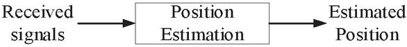
Figure 1 Estimation of position direct method.

Figure 2 Estimation of 2 steps position method.
RSS is the method used to estimate the receiver position by using the RSS of signal, which has been decreased by path loss attenuation via using the circle overlapping. A radius equal to the distance between transmitter and receiver that can be calculated by RSS. Therefore at least three circles need to be used to identify the receiver position.
The offline process needs the receiver to collect the RSS value and send back to the server to create the database that used to compare with the RSS from the online process. When the sever received the RSS value from the mobile receiver, there will be the data clustering process to separate the data cluster by using the data clustering algorithm. The data clustering algorithm, which is k-Mean clustering, will be used. Each cluster will be calculated at the centre of the cluster that used to measure the distance from each cluster to the unknown location so-called Euclidean distance as Equation (1) where is the center value of the cluster and is the RSS from the unknown location.
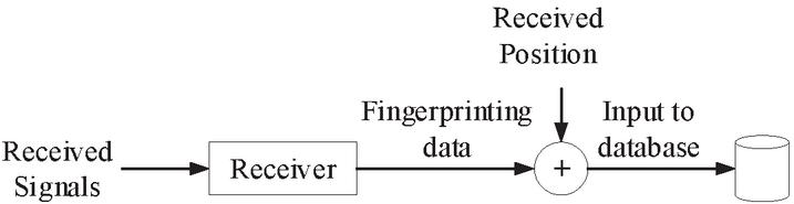
Figure 3 Fingerprinting database creation process [8].
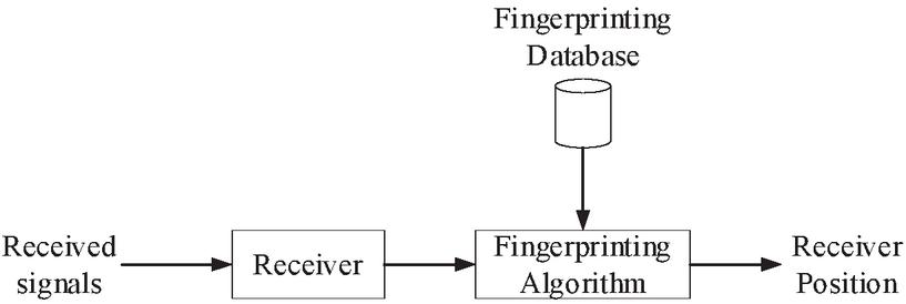
Figure 4 Fingerprinting positioning process [8].
The first step in the fingerprinting localization technique, which is the important step, is to characterize the cluster. To pre-define the centre of the cluster and calculate the Euclidean distance for each measured value by using the Equation (1). After the calculated Euclidean distance for each measured value done. The minimum Euclidean distance value can define the cluster as Equation (2) where is the cluster number.
| (1) | ||
| (2) |
After the clusters have been characterized, lead us to know which measured location and values belong to a member of which cluster. Therefore, we can re-calculate the centre of a cluster by calculating the average value of and axis by Equation (3). Then the new centre of the cluster used to characterize the cluster again. Some members of each cluster will be re-located to another and the cluster centre will be re-calculated again as per the new cluster.
| (3) |
The next step of fingerprinting localization is to measure the Euclidean distance between the RSS that carried out from the unknown location with the centre of each cluster. The minimum Euclidean distance is identified, which cluster that the RSS from the unknow location belongs to the cluster. Then after we know the cluster that the unknow location belongs to, we can proceed to estimate the position of receiver by using the k-NN algorithm.
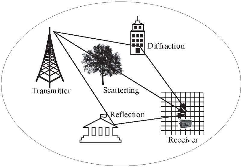
Figure 5 Localization based DTTV propagation model [8].
The positioning estimation procedure is to calculate the position of the receiver by LS method (Least Square Method) with k-Nearest Neighbor Algorithm. To calculate with the LS method can be used the Equation (4). To find the Euclidean distance where is the measured RSS and is the RSS in the database, that were carried out in the offline process.
| (4) | ||
| (5) |
The estimated location that was carried out by fingerprinting technique can be defined by the minimum Euclidean distance between the measured RSS and the RSS in the database. The estimated location can be calculated by the Equation (5). To achieve the high accuracy, there is an algorithm used to find the positioning location, which is k-Nearest Neighbor. The k-Nearest Neighbor is to increase the accuracy of position estimation by checking the k value that equal or close to each other. The k value can be defined as an odd number then find the smallest values for k number by using the Euclidean distance. The estimated position will be in x and y axis that can be calculated by the Equation (6).
| (6) |
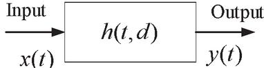
Figure 6 Linear time invariant system [5].
2.3 Clean Algorithm
According to the Clean algorithm used the channels impulse response to be cleaned. In the process, the channel impulse response can be characterized by their impulse response in the time domain or by transfer function in the frequency domain. The deconvolution in time domain waveforms can be used to determine the impulse response
| (7) | ||
| (8) | ||
| (9) |
where denoted as convolution time. The received signal is in the frequency domain can be transformed to the time domain by using the inverse Fourier transform technique
| (10) |
where is the Dirac delta function, N is number of MPCs, is amplitudes of -th MPC, is relative delays of the -th MPC and is the frequency dependent distortion on the -th echo after an interaction with the environment. The received signal is in the frequency domain that can be transformed to the time domain by using the inverse Fourier transform technique
| (11) | ||
| (12) |
where is the cross correlation between input and output, is the channel impulse response, is the channel frequency response, is the autocorrelation of input, is the cross correlation between input and output in frequency domain and is the autocorrelation of an input signal in the frequency domain. The normalized correlation can be calculated by Equation (13) and the autocorrelation can be calculated by Equation (15)
| (13) | ||
| (14) | ||
| (15) |
The channel impulse response can be estimated by cross correlation techniques by use of the relationship between the input and output signal. And for the autocorrelation functional as well. Let assume that a signal with known autocorrelation is applied to the channel , producing the output signal in the discrete time domain [5].
| (16) |
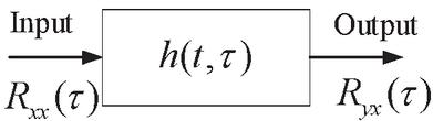
Figure 7 Input-Out relation for cross correlation [5].
The cross correlation between output and input signal is
| (17) |
where is the channel impulse response and is the autocorrelation of input signal. Hence the cross correlation between the input and output signal of the system is the convolution of the impulse response. The autocorrelation of the input signal can be viewed as the output of the channel [7, 8].
Clean algorithm is an iterative high-resolution subtractive deconvolution procedure, which is the capability of resolving dense of MPCs. They are usually unresolvable by a conventional inverse filtering. The advantage of Clean algorithm is that it models the estimated CIR (channel impulse response), which can be easily used to characterize and model delay spread, path loss and propagation channel, etc. Clean algorithm for DVB-T2 localization CIR characterization is proposed in this paper. Clean algorithm has been used in localization in UWB [7]. However, this paper present clean algorithm for DVB-T2 localization application. The objective of the clean algorithm for the DVB-T2 localization has been improved. The Clean algorithm can be used to reduce noise and decrease signal distortion. The clean algorithm process can be explained in the following detail.
| Clean Algorithm Technique [4] |
| STEP 01: Initialize normalized cross correlation between and as |
| STEP 02: Initialize normalized autocorrelation of as |
| STEP 03: Define the dirty map as |
| STEP 04: Define the clean map as |
| STEP 05: Compute and |
| STEP 06: If all threshold, go to step 10 |
| STEP 07: Clean the dirty map by |
| STEP 08: Update the cleaned map by |
| STEP 09: Go to step 5 |
| STEP 10: The CIR is then |
The algorithm above assumes independent from the generator output, measurement system, and the antenna using. Although the accuracy estimation, which is clean algorithm, is still based on the model approach. Therefore, the CIR output needs to be carefully interpreted.
The clean algorithm procedure consists of 3 parts, which are defined, compute, and clean process. The defined process is to define the variable, which are dirty map, cleaned map, cross correlation result, autocorrelation result. The second process is to find the peak and index from the cross correlation result. This result will be used to compute in clean process that will be described in the next paragraph. After the peak and index value of the cross correlation result, , was carried out then used to compare with threshold, which is 10% of . If the is less than the threshold value, the map is clean. If not, the map needs to be a loop to the clean process until the value lower than the threshold.
The first process which is define process as illustrated as Figure 8 will compute to carry out the cross correlation result of the transmitted signal with received signal and , respectively. To carry out the autocorrelation of the transmitted signal to find which time the signal will be the same with the original signal. Then define the dirty map as cross correlation of result and then define the clean map as time equal to zero.
The second process of clean algorithm, which is fine max and argmax of cross correlation result between and illustrated as Figure 8. This process will carry out the peak value of cross correlation between and . Then carry out the time that lead to peak amplitude of cross correlation between and . The threshold defined by 10 percent of peak amplitude of cross correlation between and .
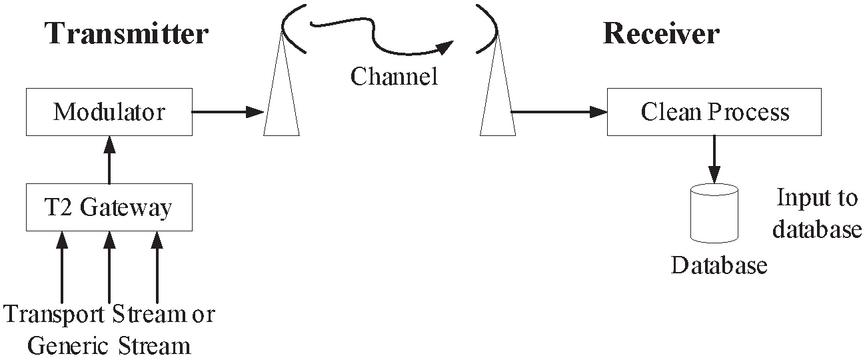
Figure 8 Block diagram of DTTV transmission model with Clean algorithm for localization system in database creation process [4].
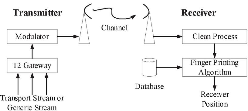
Figure 9 Block diagram of DTTV transmission model with Clean algorithm for localization system in positioning process [4].
The last process of clean algorithm, which is clean process illustrated as Figure 8 will compare the value to the threshold point. This process is important to this algorithm. If there is no function, the loop will not be stopped. If the value is lower than the threshold point means that the channel impulse response is clean. On the other hand, if the is still higher than the threshold point, the signal will run through the clean process again. The first step is to compute the compensate parameter that need to convolution to and then update the clean map.
2.4 Accuracy Analysis of Position Estimation
To analyze the estimated position of fingerprinting technique based on DTTV will analyze in terms of distance by define the measured position as , and the correct distance defined as the error distance is can be calculated by Equation (18). The distance error can be used to analyze the accuracy of the position estimation of the fingerprinting technique. The high accuracy will occur when the distance error is low.
| (18) |
3 Measurement System
The filed test area is located in Bangkok, Thailand, the distance between transmitter and tested area for 3.55 km. Transmitter high 328 m. receiver high 6 m. The tested area has been divided into a grid for 0.6 0.6 m. for 100 measured points. The measurement tool set consists of the DVB-T2 analyser equipped with a dipole antenna and tripod used to mount the dipole antenna.
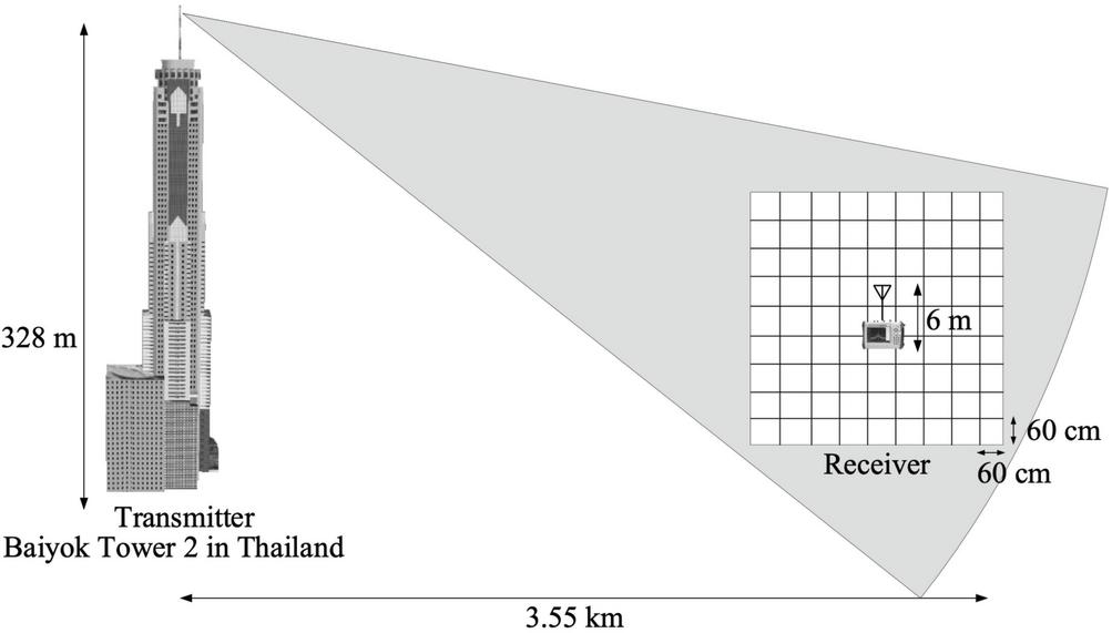
Figure 10 Receiver orientation for DTTV localization measurement.
The DTTV operators consists of 5 operators as described in Table 1 Regarding to the schematic of the DTTV transmission system illustrated as Figure 9 there are 2 parts of the system which are transmitter and receiver part. There is no modification of the transmitter part. There is only one block added to the receiver part, which is clean algorithm process that will use the received signal to clean the channel impulse response by using the channel impulse response estimation [5]. This study’s measurement scheme is based on the real measurement that has been conducted in Thailand [6] that used to compare between dirty map or estimated channel impulse response with the cleaned channel impulse response.
Table 1 Parameters of DTTV measurements
| MUX | Channel | Transmitted Frequency (MHz) | Transmitted Power (kW) |
| 1 | 26 | 514 | 4.00 |
| 2 | 36 | 594 | 4.30 |
| 3 | 40 | 626 | 4.00 |
| 4 | 44 | 658 | 3.91 |
| 5 | 52 | 722 | 4.30 |
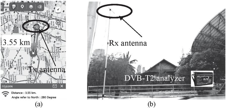
Figure 11 Real measurement location (a) distance separates between Tx and Rx antennas (b) signal received position.
4 The Result and Discussion
The measured results from 100 positions have been illustrated in Figure 13. From the results, there is a fluctuation of the field strength. The RSS value is between 50 and 65 , at the x axis represents the marked position from 1 to 100. The spectrum mask that can be read from DVB-T2 analyser illustrated in Figure 12 for each transmitter. To create the database at the offline process of the fingerprinting method, the RSS of the centre frequency has been recorded to the database.
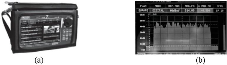
Figure 12 Measurement equipment (a) DVB-T2 analyzer (b) Example spectrum mask of MUX 1.
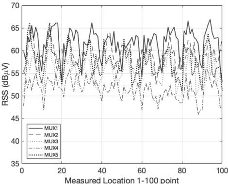
Figure 13 DTTV-RSS level each MUX1, MUX2, MUX3, MUX4 and MUX5.
From the RSS can be plotted in a contour map for each transmitter illustrated in Figures 14–18, which are NBT, ARMY1, MCOT, TPBS, and ARMY2, respectively. These RSS data can be characterized by k means clustering algorithm into each cluster for each group. Lead to the accuracy of the estimated position is increased.
After the clustering process, the contour map consists of the cluster used to identify which cluster that the RSS from unknown location belongs to. Then the next step is to proceed to estimate the positioning. This study the fingerprinting technique has been used to locate the received position. Therefore, the estimated position after the k-NN process rather accuracy. However, the RSS from the unknown location must be located. In the fingerprinting area, that has been recorded in the offline process. The recorded RSS in the offline process are between 40 to 60 dBm for five transmitters. The algorithm that has been used in this Fingerprinting technique study which is the LS method and k-NN algorithm.
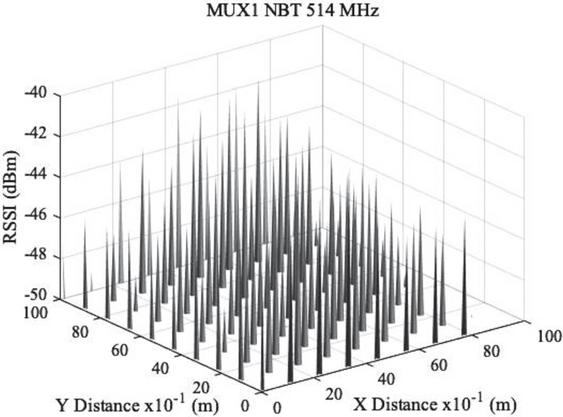
Figure 14 Three dimension of DTTV-RSS of MUX1.
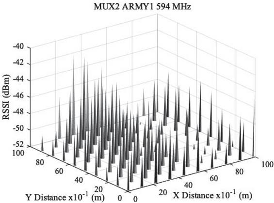
Figure 15 Three dimension of DTTV-RSS of MUX2.
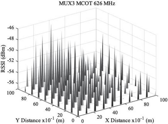
Figure 16 Three dimension of DTTV-RSS of MUX3.
The comparison between RSS for five transmitters, as illustrated in Figure 19 the average RSS is 62.38 , 57.93 , 55.39 , 50.30 , and 59.20 for MUX 1, MUX 2, MUX 3, MUX 4, and MUX 5, respectively. From these data, the MUX 1 RSS is the highest value. However, the MUX 4 RSS is the lowest value. On the other hand, as the statistical aspect, the probability distribution function shows that the highest probability of RSS belongs to MUX 4, MUX 3, MUX 2, MUX 5, and MUX 1, respectively. The cumulative distribution function of 5 MUXs, as illustrated in Figure 20.
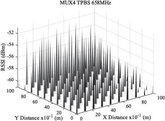
Figure 17 Three dimension of DTTV-RSS of MUX4.
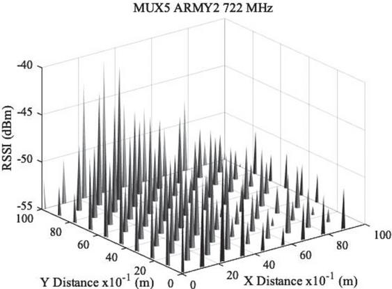
Figure 18 Three dimension of DTTV-RSS of MUX5.
According to the estimated position used the k nearest neighbor algorithm that use the minimum k value. The distance error illustrated in Table 2. The distance error for is 1.37 m. that is the maximum value from this study. By the way, the lowest error distance is , which is 1.08 m. the distance error decreased when the k value increased. The distance error illustrated in Table 2 can be described that when the k value increase leads to the distance decrease.
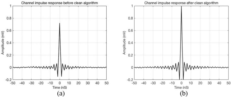
Figure 19 Received signal waveform of DTTV (a) without Clean process (b) with Clean process.
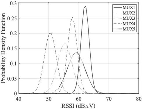
Figure 20 Comparison of PDF between MUX1, MUX2, MUX3, MUX4 and MUX5.
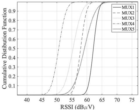
Figure 21 Comparison of CDF between MUX 1-5.
Table 4 illustrates the average distance error for k values 1, 3, 5, 7, and 9. The averaged distance error will decrease when the k value increase. The lowest distance error which is 1.20 m that carried out when and the highest distance error which is 1.33 m when .
Table 2 Distance error with clean algorithm (m)
| Distance Error (m) | |||||
| MUX | |||||
| MUX1 | 1.37 | 1.18 | 1.18 | 1.10 | 1.07 |
| MUX2 | 1.16 | 1.28 | 1.23 | 1.26 | 1.25 |
| MUX3 | 1.14 | 1.49 | 1.40 | 1.33 | 1.23 |
| MUX4 | 1.13 | 1.38 | 1.44 | 1.33 | 1.25 |
| MUX5 | 1.46 | 1.34 | 1.25 | 1.22 | 1.22 |
Table 3 Distance error without clean algorithm (m)
| Distance Error (m) | |||||
| MUX | |||||
| MUX1 | 1.65 | 1.47 | 1.48 | 1.35 | 1.30 |
| MUX2 | 1.30 | 1.34 | 1.32 | 1.33 | 1.36 |
| MUX3 | 1.44 | 1.40 | 1.40 | 1.39 | 1.35 |
| MUX4 | 1.43 | 1.36 | 1.39 | 1.37 | 1.40 |
| MUX5 | 1.39 | 1.36 | 1.38 | 1.38 | 1.42 |
Table 4 Average distance error with clean algorithm (m)
| Average Distance Error (m) | ||||
| 1.31 | 1.33 | 1.30 | 1.25 | 1.20 |
Table 5 Average distance error without clean algorithm (m)
| Average Distance Error (m) | ||||
| 1.44 | 1.39 | 1.40 | 1.36 | 1.36 |
Regarding to this study’s received signal is based on real measurement, that has been carried out from the field measurement in Bangkok Thailand [6]. MATLAB software is used to add the clean algorithm and clean signal. The averaged measurement results illustrated in Figure 13 was used to verify that this clean algorithm can be used to clean the signal. The first process of the Clean algorithm, which is the cross correlation process, defined by between and received , and the result is assumed to be channel impulse response [5] as shown in Figure 21. The received signal came with a delay time, and the cross correlation process carried out the delay time.
The cleaned channel impulse response that the delayed time has been removed. In order to get the cleaned received signal It will be used to convolve with lead to the received signal has been cleaned so-call or cleaned received signal. The autocorrelation of the input signal, has been defined as after that define the dirty and clean map as and , respectively. When compute the peak of cross correlation of and received , finished then compare all the value of to the threshold level, which is 10 percent of value. If the value is still more than the threshold, the Clean algorithm step need to be repeated until less than the threshold value.
As the compared result between before and after Clean algorithm, the delay has been removed. The increasing of amplitude is the advantage of Clean algorithm. In the Clean algorithm, the first process computes the cross correlation function between received and transmitted signals, which is normalized cross correlation. If the normal cross correlation computed, there will be a higher amplitude than this result. In order to make this calculation accuracy, the normalization needs to be used in this algorithm. Therefore, the amplitude increased from approximately 0.7 to 1.
To evaluate in term of distance error, the distance error between fingerprinting technique with Clean algorithm and without Clean algorithm described in Tables 2 and 3 respectively. The average distance error for each k value can be summarized in Tables 4 and 5 for the fingerprinting technique including and excluding Clean algorithm respectively. The averaged distanced error for all Mux and all k value from fingerprinting technique without Clean algorithm is 1.39 m on the other hand with Clean algorithm the distanced error is decreased to 1.28 m or 15.29 percent of decreasing error performance.
5 Conclusion
This study using the Signal of Opportunity, which is DTTV signal that covered 75.95% areas of Thailand excluding gap filler station. The results shown that DTTV signal can be used to locate the position of object or user on that location. In this study focuses only on outdoor environment. Due to the DTTV signal can be reduced by the channel, which are an obstruction or noise, lead to an accuracy of distance was reduced as well. Clean algorithm has been studied and the results shown that, clean algorithm can be used to reduce the noise therefore the accuracy of location increased. These results based on the actual filed measurement conducted in Bangkok, Thailand [6]. The measured raw data has been used to compute the Clean algorithm in MATLAB software by using the correlation technique used to estimate the channel impulse response and cleaned channel impulse response. The time delay was carried out by cross correlation between transmitted signal and received signal . The cleaned channel impulse response can be used to convolve to the transmitted signal to get the cleaned received signal . In the localization aspect, the fingerprinting technique has been used with K means clustering, that used to characterize the RSS. Apart from K means clustering there is a k nearest neighbour algorithm used to find the nearest position lead to the distance error was decreased from 1.39 m to 1.28 m without and with Clean algorithm respectively. The lowest distance error was carried out by k value for 9. The additional equipment is not required for the fingerprinting method with Clean algorithm in this study.
This study can be applied to the divers applications such as wireless sensor, a water level sensor system, a traffic control system, an intrusion monitoring system etc. that the obtained data location need to be sent to the controller or server therefore the performance of the foregoing application increased. Apart from this study there are the others environment such as a rural environment and indoor environment need to be studied in the future work.
References
[1] J. Huang, L. Lo Presti, R. Garello and B. Sacco, “Study of positioning methods in DVB-T single frequency networks,” Fourth International Conference on Communications and Electronics (ICCE), Hue, pp. 263–268, 2012.
[2] J. Yang, X. Wang, M. J. Rahman, S. I. Park, H. M. Kim and Y. Wu, “A New Positioning System Using DVB-T2 Transmitter Signature Waveforms in Single Frequency Networks,” in IEEE Transactions on Broadcasting, vol. 58, no. 3, pp. 347–359, 2012.
[3] R. Liu, C. Zhang and J. Song, “Line of Sight Component Identification and Positioning in Single Frequency Networks Under Multipath Propagation,” in IEEE Transactions on Broadcasting, vol. 65, no. 2, pp. 220–233, 2019.
[4] K. Koonchiang, D. Arpasilp and S. Promwong, “Performance Evaluation of UWB-BAN with Friis’s Formula and CLEAN Algorithm,” In: Park J., Ng JY., Jeong HY., Waluyo B. (eds) Multimedia and Ubiquitous Engineering. Lecture Notes in Electrical Engineering, Springer, Dordrecht, vol. 240, 2013.
[5] J. G. Proakis and D. G. Manolakis, “Digital Signal Processing: Principles, Algorithmns and Applications,” 4ed. New Jersey: Pearson Education Inc, 2007.
[6] N. Suwansukho and S. Promwong, “Experimental Study of DVB-T2 Threshold,” 2019 Joint International Conference on Digital Arts, Media and Technology with ECTI Northern Section Conference on Electrical, Electronics, Computer and Telecommunications Engineering (ECTI DAMT-NCON), Nan, Thailand, pp. 114–118, 2019.
[7] A. Muqaibel, A. Safaai-Jazi, B. Woerner and S. Riad, “UWB channel impulse response characterization using deconvolution techniques,” The 2002 45th Midwest Symposium on Circuits and Systems, 2002. MWSCAS-2002., Tulsa, OK, USA, pp. III–605, 2002.
[8] E. C. L. Chan and G. Baciu, “Introduction to wireless localization with iPhone sdk example,” 2012 John Wiley & Sons Singapore Pte. Ltd.
[9] T. C. Liu, D. I. Kim and R. G. Vaughan, “A high-resolution, multi-template deconvolution algorithm for time-domain UWB channel characterization,” in Canadian Journal of Electrical and Computer Engineering, vol. 32, no. 4, pp. 207–213, 2007.
[10] W. Yang and Z. Naitong, “A New Multi-Template CLEAN Algorithm for UWB Channel Impulse Response Characterization,” 2006 International Conference on Communication Technology, Guilin, pp. 1–4, 2006.
[11] Z. Sharif and A. Z. Sha’ameri, “The Application of Cross Correlation Technique for Estimating Impulse Response and Frequency Response of Wireless Communication Channel,” 2007 5th Student Conference on Research and Development, Selangor, Malaysia, pp. 1–5, 2007.
[12] A. Chandra et al., “CLEAN algorithms for intra-vehicular time-domain UWB channel sounding,” 2015 International Conference on Pervasive and Embedded Computing and Communication Systems (PECCS), Angers, France, pp. 1–6, 2015.
[13] W. Yang and Z. Naitong, “A New Multi-Template CLEAN Algorithm for UWB Channel Impulse Response Characterization,” 2006 International Conference on Communication Technology, Guilin, pp. 1–4, 2006.
[14] T. C. Liu, D. I. Kim and R. G. Vaughan, “A High-Resolution, Multi-Template Deconvolution Algorithm for Time-Domain UWB Channel Characterization,” 2007 Canadian Conference on Electrical and Computer Engineering, Vancouver, BC, pp. 1183–1186, 2007.
[15] S. M. Yano, “Investigating the ultra-wideband indoor wireless channel,” Vehicular Technology Conference. IEEE 55th Vehicular Technology Conference. VTC Spring 2002 (Cat. No.02CH37367), Birmingham, AL, USA, pp. 1200–1204, vol.3, 2002.
[16] L. R. N. Ferreira, L. T. Pereira and R. L. de S. da. Silva, “Immersive Mobile Telepresence Systems: A Systematic Literature Review,” Journal of Mobile Multimedia, vol. 15-3, pp. 255–270, River Publishers, 2020.
[17] M. Darnell, “Techniques for the real-time identification of radio channels,” 1994 International Conference on Control – Control ’94., Coventry, UK, vol. 1, pp. 543–548, 1994.
[18] X. Wang, Y. Wu, B. Caron, B. Ledoux and S. Lafleche, “A channel characterization technique using frequency-domain pilot time-domain correlation method for DVB-T systems,” 2003 IEEE International Conference on Consumer Electronics, 2003. ICCE., Los Angeles, CA, USA, pp. 294–295, 2003.
[19] P. Bello, “Characterization of Randomly Time-Variant Linear Channels,” in IEEE Transactions on Communications Systems, vol. 11, no. 4, pp. 360–393, 1963.
[20] G. Pecoraro, E. Cianca, S. Di Domenico and M. De Sanctis, “LTE Signal Fingerprinting Device-Free Passive Localization Robust to Environment Changes,” 2018 Global Wireless Summit (GWS), Chiang Rai, Thailand, pp. 114–118, 2018.
[21] J. Sangthong, S. Promwong and P. Supanakoon, “Comparison of UWB fingerprinting with vertical and horizontal polarizations for indoor localization,” ECTI-CON2010: The 2010 ECTI International Confernce on Electrical Engineering/Electronics, Computer, Telecommunications and Information Technology, Chiang Mai, pp. 588–592, 2010.
[22] W. Vinicchayakul and S. Promwong, “Improvement of fingerprinting technique for UWB indoor localization,” The 4th Joint International Conference on Information and Communication Technology, Electronic and Electrical Engineering (JICTEE), Chiang Rai, pp. 1–5, 2014.
[23] W. Vinicchayakul and S. Promwong, “Performance comparison between UWB and NB propagation models for an indoor localization,” The 20th Asia-Pacific Conference on Communication (APCC2014), Pattaya, pp. 299–302, 2014.
[24] J. Thongkam, P. Supanakoon and S. Promwong, “Indoor Wireless Sensor Network Localization Using RSSI Based Weighting Algorithm Method for Short Range Wireless Communication,” 2018 International Electrical Engineering Congress (iEECON), Krabi, Thailand, pp. 1–4, 2018.
[25] K. Lorvannger, D. Lakanchanh, T. Tiengthong and S. Promwong, “WLAN Localization Measurement and Analysis Using RSS and TOA Positioning Methods,” 2018 Global Wireless Summit (GWS), Chiang Rai, Thailand, pp. 319–322, 2018.
[26] L. Thammavong, K. Khongsomboon and S. Promwong, “Quantitative Evaluation of Zigbee Localization Based on Weighted Centroid with Quadratic Means,” 2018 Global Wireless Summit (GWS), Chiang Rai, Thailand, pp. 323–326, 2018.
[27] J. Thongkam, P. Supanakoon and S. Promwong, “Evaluation of Indoor Localization with Range-Free Weighted Localization Algorithm,” 2018 Global Wireless Summit (GWS), Chiang Rai, Thailand, pp. 11–14, 2018.
Biographies
Sathaporn Promwong has received a Ph.D. degree from Tokyo Institute of Technology (TIT), Tokyo, Japan in communications and integrated systems, and received a M.E. degree and B.Ind.Tech degree from King Mongkut’s Institute of Technology Ladkrabang (KMITL), Bangkok, Thailand in electrical engineering, and electronic technology, respectively. In the present he is a Chair of IEEE Broadcast Technology Society (BTS) Thailand Chapter. He is a member of IEEE, IEICE and ECTI. Dr. Sathaporn’s research interests on digital broadcasting technology, wireless communication system, antenna and radio wave propagation and ultra wideband (UWB) technology.

Nattapan Suwansukho has received B.E. degree in electronics and telecommunication engineering from Pathumwan Institute of Technology (PIT) and M.E. degree in telecommunication engineering from King Mongkut’s Institute of Technology Ladkrabang (KMITL). Now he is a doctoral candidate at the school of engineering, KMITL. His research interests in the DTTV technology and DTTV localization measurement and broadcasting technology.
Journal of Mobile Multimedia, Vol. 18_3, 821–844.
doi: 10.13052/jmm1550-4646.18318
© 2022 River Publishers