Performance Analysis of Orthogonal Gradient Sign Algorithm Using Spline-based Hammerstein Model for Smart Application

Suchada Sitjongsataporn^1,* and Sethakarn Prongnuch²

¹Department of Electronic Engineering, Mahanakorn Institute of Innovation (MII), Faculty of Engineering and Technology, Mahanakorn University of Technology, 140 Cheumsamphan Rd., Nongchok, Bangkok, Thailand
²Department of Robotics Engineering, Faculty of Industrial Technology, Suan Sunandha Rajabhat University, 1 U-Thong Nok Rd., Dusit, Bangkok, Thailand
E-mail: ssuchada@mut.ac.th; sethakarn.pr@ssru.ac.th
*Corresponding Author

Received 30 July 2021; Accepted 20 January 2022; Publication 17 March 2022

Abstract

This paper presents a spline-based Hammerstein model for adaptive filtering based on a sign algorithm with the normalised orthogonal gradient algorithm. Spline-based Hammerstein architecture consists of an interpolation spline-based adaptive lookup table in the part of nonlinear filter and an adaptive finite impulse response filter used in the part of linear filter. Hammerstein spline adaptive filter (HSAF) is a nonlinear filter for the nonlinear systems among the advantages in the low computational cost and high performance. An adaptive lookup table and spline control points are determined and derived with the orthogonal gradient-based mechanism. Performance analysis in terms of convergence properties and mean square analysis based on the mean square error (MSE) constraint are proven by using the Taylor series expansion of the estimation error in the form of the excess MSE. Experimental results indicate the robust performance of the proposed algorithm can provide the better performance than the other models based on the conventional least mean square Hammerstein spline adaptive filtering algorithm.

Keywords: Hammerstein model, spline adaptive filtering, sign algorithm, orthogonal gradient adaptive algorithm, nonlinear systems.

1 Introduction

Recently, the nonlinear system identification has been interestingly applied to solve the system modelling problem. A class of spline-based adaptive filtering (SAF) structure [1–4] has been presented. SAF is a type of nonlinear spline adaptive filter detailed in [2], which has been presented the performance in terms of adaptive learning for the nonlinear system modelling [3]. Normalised version of least mean square for SAF has been proposed in [4, 5] for the nonlinear system identification.

SAF architecture has been modified in several fields of engineering such as the nonlinear system identification using the infinite impulse response (IIR) [6, 7] against impulsive noise [8], system identification [9] and multilayer feedforward networks [10]. SAF based on IIR nonlinear filtering is proposed in order to solve the Wiener nonlinear system identification in [6]. The set-membership framework and least-M estimate approach has been presented in the combination method [8] for achieving the effective suppression and fast convergence on the impulsive noise. Normalised version of orthogonal gradient-based adaptive applied for SAF [9] has been presented in the system identification. An adaptive spline with activation function based on the neural network [10] is presented due to solve in the data processing real-time problems.

However, Hammerstein model based on SAF (HSAF) is a kind of nonlinear model applied in several nonlinear systems [11, 12] such as the Hammerstein on cubic SAF [11] and the digital cancellation in full duplex [12]. HSAF based on the stochastic gradient descent algorithm with the normalised version of least mean square (NLMS) algorithm has been presented in [13].

Hammerstein spline-based adaptive filter (HSAF) architecture consists of an interpolation spline-based adaptive lookup table in the part of nonlinear filter and an adaptive finite impulse response (FIR) filter in the part of linear filter. HSAF has been derived with a memory-less function based on a uniform cubic spline function [11], which the results reveal that the proposed filter can properly apply during the learning process using the gradient approach. For a self-interference canceller, a HSAF algorithm applied for full-duplex devices has been proposed to reduce the complexity compared to the common solution [12]. Performance results from in-band full-duplex prototype demonstrated that it can obtain the same performance with low computational complexity.

For the fast convergence, the orthogonal gradient-based adaptive algorithm (OGA) has been verified in [14, 15]. Based on the orthogonal projection, the author in [15] has been derived with the greedy approach for the convergence analysis. As a remark on the advantage of Hammerstein spline-based filtering and fast convergence of OGA-based, it is inspired that the adaptation process of coefficients can be applied during learning with low computational complexity.

This paper is organised as follows. System model and a proposed Hammerstein spline-based adaptive filtering based on the sign algorithm and normalised orthogonal gradient-based adaptive algorithm are described in Section 2. Convergence properties in terms of stability and mean square analysis are derived in Section 3. Numerical results are shown in Section 4. Conclusion is summarised in Section 5. In this paper, vectors are defined by the boldface lowercase letters. Matrix is obtained with boldface capital letter. In addition, the floor operator, absolute value and transpose operator stand for $\lfloor \cdot \rfloor$, $|\cdot |$ and ${(\cdot )}^T$, respectively.

2 Proposed Spline-based Hammerstein Algorithm and System Model

2.1 Spline Interpolation

General type of piece-wise polynomials in the spline interpolation under the smooth and continuity constraints are applied to interpolate the input [1]. That means a nonlinear system can be modelled with low-order piece-wise polynomials through a set of adaptive control points in the system.

Therefore, the spline curve is a combination of spline segments between knots. The particular area between the i${}^{t\mathit{}h}$ and i+1${}^{t\mathit{}h}$ knot is called the ‘i${}^{t\mathit{}h}$-span’ as

$u(k)$	$={\displaystyle \frac{x(k)}{\mathrm{△}x}}-\lfloor {\displaystyle \frac{x(k)}{\mathrm{△}x}}\rfloor ,$	(1)
$i(k)$	$=\lfloor {\displaystyle \frac{x(k)}{\mathrm{△}x}}\rfloor +{\displaystyle \frac{Q-1}{2}},$	(2)

where $x(k)$ is the input signal, $\mathrm{△}x$ is the uniform space between successive knots and Q is the number of knots.

The spline interpolation output is given with the matrix notation as [2]

$${\mathbf{\text{s}}}_i(k)=\mathbf{\text{u}}{(k)}^T\mathbf{\text{C}}\mathbf{\text{q}}(k),$$

(3)

where the output vector ${\mathbf{\text{s}}}_i(k)$ sorted from the span index i in the present iteration k, $0\le i\le Q-1.$ A real-valued control points vector is as $\mathbf{\text{q}}(k)\in {ℝ}^{Q+1}$ and $\mathbf{\text{u}}{(k)}^{\mathbf{\text{T}}}\mathbf{\text{C}}$ defines the matrix multiplication between the spline basis matrix and vector $\mathbf{\text{u}}(k)\in {ℝ}^{(p+1)\times 1}$ as

$\mathbf{\text{q}}(k)$	$={[q_0{q}_1\mathrm{\dots }{q}_{Q-1}]}^T,$	(4)
$\mathbf{\text{u}}(k)$	$={[u^P(k)u^{P-1}(k)\mathrm{\dots }u(k)\mathrm{\hspace{0.25em}1}]}^T,$	(5)

where P denotes a piece-wise degree of spline curve.

Figure 1 Spline-based Hammerstein model, where $\mathit{\text{P}}=3$.

2.2 Spline-based Hammerstein Model

Splined-interpolated adaptive lookup table and FIR filter architecture is depicted in Figure 1, where $\mathbf{\text{x}}(k)$ is the input signal and $\mathbf{\text{y}}(k)$ is the output signal as

$$y(k)=\mathbf{\text{w}}{(k)}^T{\mathbf{\text{s}}}_i(k),$$

(6)

where $\mathbf{\text{w}}(k)\in {ℝ}^{M\times 1}$ is the FIR of the linear filter as

$$\mathbf{\text{w}}(k)={\left[w_0(k)w_1(k)\mathrm{\dots }{w}_{M-1}(k)\right]}^T,$$

(7)

where M is the number of tap of coefficient vector.

According to the estimating unknown parameters, the error signal e$(k)$ is considered the adaptive linear filter $\mathbf{\text{w}}(k)$ and the spline control points $\mathbf{\text{q}}(k)$ as

$$e(k)=d(k)-y(k)=d(k)-\mathbf{\text{w}}{(k-1)}^T{\mathbf{\text{s}}}_i(k),$$

(8)

where $d(k)$ denotes the desired signal.

2.3 Proposed Orthogonal Gradient Sign Algorithm for Spline-based Hammerstein Adaptive Filtering

By estimating the weights of $\mathbf{\text{w}}(k)$ and $\mathbf{\text{q}}(k)$ in order to minimise the error $e(k)$ can be done by using the gradient descent-based algorithm, the cost function is minimised the squared error as [3, 11]

$$\mathbf{\text{J}}(\mathbf{\text{w}},\mathbf{\text{q}})=\frac{\mathbf{\text{1}}}{\mathbf{\text{2}}}\underset{\mathbf{\text{w,q}}}{\mathbf{min}}\{{|e(k)|}^{\mathbf{\text{2}}}\},$$

(9)

where $e(k)$ is given in (8).

Differentiating the cost function in (9) with respect to (w.r.t) $\mathbf{\text{w}}(k)$ and $\mathbf{\text{q}}(k)$, we get

$\mathbf{\nabla }{\mathbf{\text{J}}}_{\mathbf{\text{w}}}$	$={\displaystyle \frac{\partial \mathbf{\text{J}}(\mathbf{\text{w}},\mathbf{\text{q}})}{\partial \mathbf{\text{w}}(k)}}={\mathbf{\text{s}}}_i(k)\cdot e(k),$	(10)
$\mathbf{\nabla }{\mathbf{\text{J}}}_{\mathbf{\text{q}}}$	$={\displaystyle \frac{\partial \mathbf{\text{J}}(\mathbf{\text{w}},\mathbf{\text{q}})}{\partial \mathbf{\text{q}}(k)}}=-\mathbf{\text{u}}{(k)}^T\cdot \mathbf{\text{C}}\cdot \mathbf{\text{w}}(k)\cdot e(k).$	(11)

Consequently, the proposed coefficient vector $\mathbf{\text{w}}(k)$ based on the sign version of the normalised orthogonal gradient adaptive (SNOGA) algorithm is verified by

$$\mathbf{\text{w}}(k)=\mathbf{\text{w}}(k-1)+{\mu }_w\cdot {\mathbf{\text{d}}}_w(k),$$

(12)

where ${\mathbf{\text{d}}}_w(k)$ is the vector direction of linear filter $\mathbf{\text{w}}(k)$ as

$${\mathbf{\text{d}}}_w(k)={\mathbf{\text{d}}}_w(k-1)+{\lambda }_w\cdot {\mathbf{\text{g}}}_w(k),$$

(13)

where ${\lambda }_w$ is the forgetting factor for $\mathbf{\text{w}}(k)$.

The negative gradient ${\mathbf{\text{g}}}_w(k)$ of $\mathbf{\text{w}}(k)$ is expressed by taking the partial derivative of the cost function in (10) w.r.t $\mathbf{\text{w}}(k)$ as given in (12) as

${\mathbf{\text{g}}}_w(k)$	$={\lambda }_w(k)\cdot {\mathbf{\text{g}}}_w(k)-{\displaystyle \frac{\partial \mathbf{\text{J}}(\mathbf{\text{w}},\mathbf{\text{q}})}{\partial \mathbf{\text{w}}(k)}},$	(14)
$\therefore {\mathbf{\text{g}}}_w(k)$	$={\lambda }_w(k)\cdot {\mathbf{\text{g}}}_w(k)-{\mathbf{\text{s}}}_i(k)\cdot \mathrm{sgn}\{e(k)\},$	(15)

where $\mathrm{sgn}\{\cdot \}$ is the sign operator.

Therefore, the proposed control points $\mathbf{\text{q}}(k)$ based on the sign version of NOGA is similarly written by

$$\mathbf{\text{q}}(k)=\mathbf{\text{q}}(k-1)+{\mu }_q\cdot {\mathbf{\text{d}}}_q(k),$$

(16)

where ${\mathbf{\text{d}}}_q(k)$ is the directional vector of control points $\mathbf{\text{q}}(k)$ as

$${\mathbf{\text{d}}}_q(k)={\mathbf{\text{d}}}_q(k-1)+{\lambda }_q\cdot {\mathbf{\text{g}}}_q(k),$$

(17)

where ${\lambda }_q$ is the forgetting factor for $\mathbf{\text{q}}(k)$.

The gradient vector ${\mathbf{\text{g}}}_q(k)$ of $\mathbf{\text{q}}(k)$ can be obtained similarly as

${\mathbf{\text{g}}}_q(k)$	$={\lambda }_q(k)\cdot {\mathbf{\text{g}}}_q(k)-{\displaystyle \frac{\partial \mathbf{\text{J}}(\mathbf{\text{w}},\mathbf{\text{q}})}{\partial \mathbf{\text{q}}(k)}},$	(18)
$\therefore {\mathbf{\text{g}}}_q(k)$	$={\lambda }_q(k)\cdot {\mathbf{\text{g}}}_q(k)-\mathbf{\text{u}}{(k)}^T\cdot \mathbf{\text{C}}\cdot \mathbf{\text{w}}(k)\cdot e(k),$	(19)

As shown in [14, 15], the forgetting factor ${\lambda }_w(k)$ of $\mathbf{\text{w}}(k)$ and ${\lambda }_q(k)$ of $\mathbf{\text{q}}(k)$ lie on the orthogonal projection of the present gradient vectors${\mathbf{\text{g}}}_w(k)$, ${\mathbf{\text{g}}}_q(k)$ and the previous directional vectors ${\mathbf{\text{d}}}_w(k-1)$, ${\mathbf{\text{d}}}_q(k-1)$ as

${\lambda }_w(k)$	$={\displaystyle \frac{{\mathbf{\text{d}}}_w{(k-1)}^T{\mathbf{\text{g}}}_w(k-1)}{{\mathbf{\text{d}}}_w{(k)}^T{\mathbf{\text{d}}}_w(k-1)}},$	(20)
${\lambda }_q(k)$	$={\displaystyle \frac{{\mathbf{\text{d}}}_q{(k-1)}^T{\mathbf{\text{g}}}_q(k-1)}{{\mathbf{\text{d}}}_q{(k)}^T{\mathbf{\text{d}}}_q(k-1)}}.$	(21)

According to the estimation of memory model [1], it is seen that the spline control points are independent on the linear filter $\mathbf{\text{w}}(k)$, so the memory is used after the nonlinearity.

During the adaptation process, the adaptive linear filter $\mathbf{\text{w}}(k)$ and the spline control points $\mathbf{\text{q}}(k)$ are updated recursively in parallel as summarised in Table 2.3.

Proposed sign normalised orthogonal gradient adaptive algorithm for Hammerstein spline-based adaptive filtering (SNOGA-HSAF) Initialise: $(0)={\delta }_w\cdot {[\mathrm{1\hspace{0.25em}0}\mathrm{\dots }\mathrm{\hspace{0.25em}0}]}^T$, $\mathbf{\text{q}}(0)={[\mathrm{1\hspace{0.25em}0}\mathrm{\dots }\mathrm{\hspace{0.25em}0}]}^T$

${\mathbf{\text{d}}}_w(0)={\mathbf{\text{d}}}_q(0)={\mathbf{\text{g}}}_q(0){[\mathrm{1\hspace{0.25em}0}\mathrm{\dots }\mathrm{\hspace{0.25em}0}]}^T,\mathrm{△}x=0.2$

For $\mathrm{k}=1,2,\mathrm{\dots }$

For $u(k)={\displaystyle \frac{x(k)}{\mathrm{△}x}}-\lfloor {\displaystyle \frac{x(k)}{\mathrm{△}x}}\rfloor$

For $i(k)=\lfloor {\displaystyle \frac{x(k)}{\mathrm{△}x}}\rfloor +{\displaystyle \frac{Q-1}{2}}$

For $\mathbf{\text{u}}(k)={[u^P(k)u^{P-1}(k)\mathrm{\dots }u(k)\mathrm{\hspace{0.25em}1}]}^T$

For ${\mathbf{\text{s}}}_i(k)=\mathbf{\text{u}}{(k)}^T\mathbf{\text{C}}\mathbf{\text{q}}(k)$

For $y(k)=\mathbf{\text{w}}{(k)}^T{\mathbf{\text{s}}}_i(k)$

For $e(k)=d(k)-\mathbf{\text{w}}{(k-1)}^T{\mathbf{\text{s}}}_i(k)$

For ${\mathbf{\text{g}}}_w(k)={\lambda }_w(k)\cdot {\mathbf{\text{g}}}_w(k)-{\mathbf{\text{s}}}_i(k)\cdot \mathrm{sgn}\{e(k)\}$

For ${\mathbf{\text{d}}}_w(k)={\lambda }_w\cdot {\mathbf{\text{d}}}_w(k)-{\mathbf{\text{g}}}_w(k-1)$

For $\mathbf{\text{w}}(k)=\mathbf{\text{w}}(k-1)+{\mu }_w\cdot {\mathbf{\text{d}}}_w(k)$

For ${\mathbf{\text{g}}}_q(k)={\lambda }_q(k)\cdot {\mathbf{\text{g}}}_q(k)-\mathbf{\text{u}}{(k)}^T\cdot \mathbf{\text{C}}\cdot \mathbf{\text{w}}(k)\cdot e(k)$

For ${\mathbf{\text{d}}}_q(k)={\lambda }_q\cdot {\mathbf{\text{d}}}_q(k)-{\mathbf{\text{g}}}_q(k-1)$

For $\mathbf{\text{q}}(k)=\mathbf{\text{q}}(k-1)+{\mu }_q\cdot {\mathbf{\text{d}}}_q(k)$

For ${\lambda }_w(k)={\displaystyle \frac{{\mathbf{\text{d}}}_w{(k-1)}^T{\mathbf{\text{g}}}_w(k-1)}{{\mathbf{\text{d}}}_w{(k)}^T{\mathbf{\text{d}}}_w(k-1)}}$

For ${\lambda }_q(k)={\displaystyle \frac{{\mathbf{\text{d}}}_q{(k-1)}^T{\mathbf{\text{g}}}_q(k-1)}{{\mathbf{\text{d}}}_q{(k)}^T{\mathbf{\text{d}}}_q(k-1)}}$

end

3 Convergence Properties

In order to obtain the optimal performance, the minimisation on the error of filters can be maintained an adaptive learning rate of algorithm.

3.1 Stability

Let us introduce the approximation form of iterative learning orthogonal gradient-based sign algorithm for adaptive FIR spline-based Hammerstein filtering $\mathbf{\text{w}}(k)$ as

$$\mathbf{\text{w}}(k)=\mathbf{\text{w}}(k-1)+{\mu }_w\cdot {\mathbf{\text{s}}}_i(k)\cdot \mathrm{sgn}\{e(k)\},$$

(22)

where $\mathrm{sgn}\{e(k)\}$ denotes the sign of error parameter.

The convergence property of adaptive FIR filtering $\mathbf{\text{w}}(k)$ in (22) can be calculated by the Taylor series expansion of the estimation error signal $e(k+1)$ as

$$e(k+1)\approx e(k)+\frac{\partial e(k)}{\partial \mathbf{\text{w}}(k)}\cdot \mathrm{△}\mathbf{\text{w}}(k),$$

(23)

where $\frac{\partial e(k)}{\partial \mathbf{\text{w}}(k)}\cdot \mathrm{△}\mathbf{\text{w}}(k)$ is the first order of Taylor series expansion and $\mathrm{△}\mathbf{\text{w}}(k)$ is the difference of $\mathbf{\text{w}}(k)$ as

$$\mathrm{△}\mathbf{\text{w}}(k)=\mathbf{\text{w}}(k)-\mathbf{\text{w}}(k-1)\approx {\mu }_w\cdot {\mathbf{\text{s}}}_i(k)\cdot \mathrm{sgn}\{e(k)\},$$

(24)

and the estimation a priori error $e(k)$ is defined as

$$e(k)=d(k)-\mathbf{\text{w}}{(k-1)}^T{\mathbf{\text{s}}}_i(k).$$

(25)

Differentiating $e(k)$ in (25) with respect to $\mathbf{\text{w}}(k)$, we arrive at

$$\frac{\partial e(k)}{\partial \mathbf{\text{w}}(k)}=-{\mathbf{\text{s}}}_i(k),$$

(26)

and substitution (24) and (26) in (23), we get

$e(k+1)\approx e(k)-{\mu }_w\cdot {\mathbf{\text{s}}}_i{(k)}^T{\mathbf{\text{s}}}_i(k)\cdot \mathrm{sgn}\{e(k)\}.$

(27)

By taking the norm at both sides of (27), we carry out with the simple manipulations as

$$e(k+1)\approx e(k)\{1-{\mu }_w\cdot {\mathbf{\text{s}}}_i{(k)}^T{\mathbf{\text{s}}}_i(k)\}.$$

(28)

Let assume that $|e(k+1)|<|e(k)|$ in order to achieve the convergence, we arrive at

$$1=1-{\mu }_w\cdot {\mathbf{\text{s}}}_i{(k)}^T{\mathbf{\text{s}}}_i(k),$$

(29)

that indicates the bound on the learning rate of step-size ${\mu }_w$ of $\mathbf{\text{w}}(k)$ as

$$0<{\mu }_w<\frac{1}{{\mathbf{\text{s}}}_i{(k)}^T{\mathbf{\text{s}}}_i(k)}.$$

(30)

It is seen that all quantities following in (30) are positive.

Correspondingly, the approximation form of adaptive control points $\mathbf{\text{q}}(k)$ on the sign orthogonal gradient algorithm is updated by

$$\mathbf{\text{q}}(k)=\mathbf{\text{q}}(k-1)+{\mu }_q\cdot \mathbf{\text{u}}{(k)}^T\cdot \mathbf{\text{C}}\cdot \mathbf{\text{w}}(k)\cdot \mathrm{sgn}\{e(k)\}.$$

(31)

So, we can determine a bound on the choice of ${\mu }_q$ by the first order of Taylor series expansion of error $e(k)$ related with the adaptive control points $\mathbf{\text{q}}(k)$ as

$$e(k+1)\approx e(k)+\frac{\partial e(k)}{\partial \mathbf{\text{q}}(k)}\cdot \mathrm{△}\mathbf{\text{q}}(k),$$

(32)

where $\frac{\partial e(k)}{\partial \mathbf{\text{q}}(k)}\cdot \mathrm{△}\mathbf{\text{q}}(k)$ is the first order of Taylor series expansion and $\mathrm{△}\mathbf{\text{q}}(k)$ is the difference of previous and present of $\mathbf{\text{q}}(k)$ in (31) as

$$\mathrm{△}\mathbf{\text{q}}(k)=\mathbf{\text{q}}(k)-\mathbf{\text{q}}(k-1)\approx {\mu }_q\cdot \mathbf{\text{u}}{(k)}^T\cdot \mathbf{\text{C}}\cdot \mathbf{\text{w}}(k)\cdot \mathrm{sgn}\{e(k)\}.$$

(33)

Substituting ${\mathbf{\text{s}}}_{\mathbf{\text{i}}}(k)$ in (3) into (25), we have

$$e(k)=d(k)-\mathbf{\text{w}}{(k-1)}^T\{\mathbf{\text{u}}(k)\cdot \mathbf{\text{C}}\cdot \mathbf{\text{ q}}(k)\}.$$

(34)

Taking the derivative on $e(k)$ in (34) with respect to $\mathbf{\text{q}}(k)$, that is

$$\frac{\partial e(k)}{\partial \mathbf{\text{q}}(k)}=-\mathbf{\text{w}}{(k-1)}^T\{\mathbf{\text{u}}(k)\cdot \mathbf{\text{C}}\}.$$

(35)

After the simple manipulations, the estimation error $e(k)$ can be obtained as

$e(k+1)$	$\approx e(k)-{\mu }_q\cdot \mathbf{\Psi }{(k)}^T\cdot \mathbf{\Psi }(k)\cdot \mathrm{sgn}\{e(k)\},$	(36)
$\mathbf{\Psi }(k)$	$=\mathbf{\text{w}}{(k-1)}^T\cdot \mathbf{\text{C}}\cdot \mathbf{\text{u}}(k).$	(37)

By determining the convergence of error in (36) following in (8), we have

$$1=1-{\mu }_q\cdot \mathbf{\Psi }{(k)}^T\mathbf{\Psi }(k),$$

(38)

that imposes a bound on the learning rate ${\mu }_q$ as

$$0<{\mu }_w<\frac{1}{\mathbf{\Psi }{(k)}^T\mathbf{\Psi }(k)}.$$

(39)

3.2 Mean Square Analysis

The purpose of this section is to derive the mean square error performance of orthogonal gradient-based sign algorithm on the spline-based Hammerstein filtering at the steady-state. The mean square analysis is separated to the first case of adaptive FIR linear filter $\mathbf{\text{w}}(k)$ and then the spline control points $\mathbf{\text{q}}(k)$.

The excess mean square error (EMSE) is considered by following these parameters. A posterior error $e_p(k)$ imposed on the error of system. A priori error $e_{p_w}$$(k)$ is determined when the adaptive FIR linear filter $\mathbf{\text{w}}(k)$ is updated, while fixing the spline control points $\mathbf{\text{q}}(k)$. Similarly, a posteriori error $e_{p_q}(k)$ is imposed on the adaptive control points $\mathbf{\text{q}}(k)$, while fixing the linear filter $\mathbf{\text{w}}(k)$.

According to the mathematical derivation, these assumptions are introduced.

Assumption 1: The estimated error vector ${\mathit{\zeta }}_{\mathbf{\text{w}}}$(k) involved with the adaptive linear filter $\mathbf{\text{w}}(k)$ is under the circumstance of independent and identically distributed (i.i.d) condition with the finite variance and zero mean.

The estimated error vector ${\mathit{\zeta }}_{\mathbf{\text{w}}}$(k) is determined with the adaptive linear filter $\mathbf{\text{w}}(k)$ as

$${\mathit{\zeta }}_{\mathbf{\text{w}}}(k+1)={\mathit{\zeta }}_{\mathbf{\text{w}}}(k)-\mathrm{\Delta }\mathbf{\text{w}}(k),$$

(40)

And $\mathrm{\Delta }\mathbf{\text{w}}(k)$ is given as

$$\mathrm{△}\mathbf{\text{w}}(k)\approx {\mu }_w\cdot {\mathbf{\text{s}}}_i(k)\cdot \mathrm{sgn}\{e_{p_w}(k)\},$$

(41)

where $e_{p_w}(k)$ denotes a posteriori error related with $\mathbf{\text{w}}(k)$.

Assumption 2: We assume that

$$E\{{\parallel {\mathit{\zeta }}_{\mathbf{\text{w}}}(k+1)\parallel }^2\}\approx E\{{\parallel {\mathit{\zeta }}_{\mathbf{\text{w}}}(k)\parallel }^2\},k\to \mathrm{\infty }.$$

Following Assumption 2, we can consider the energies of error in (40) by taking the expectation of square at both sides of (40) as

${\parallel {\mathit{\zeta }}_{\mathbf{\text{w}}}(k+1)\parallel }^2$	$={\parallel {\mathit{\zeta }}_{\mathbf{\text{w}}}(k)\parallel }^2-2{\mu }_w\cdot {\mathit{\zeta }}_{\mathbf{\text{w}}}(k-1)\cdot {\mathbf{\text{s}}}_i(k)\cdot \mathrm{sgn}\{e_{p_w}(k)\}$
	$\mathrm{\hspace{1em}}+\mu _w{}^2{\parallel {\mathbf{\text{s}}}_i(k)\cdot \mathrm{sgn}\{e_{p_w}(k)\}\parallel }^2,$	(42)

We obtain

$$2{\mathbf{\text{s}}}_i{(k)}^T\cdot {\mathit{\zeta }}_{\mathbf{\text{w}}}(k)\cdot \mathrm{sgn}\{e_{p_w}(k)\}={\mu }_w\cdot {\mathbf{\text{s}}}_i{(k)}^T\cdot {\mathbf{\text{s}}}_i(k)\cdot {|e_{p_w}(k)|}^2,$$

(43)

We assume that a posteriori error $e_{p_w}(k)$ associated with the estimated error vector ${\mathit{\zeta }}_{\mathbf{\text{w}}}(k)$ of the adaptive FIR linear filtering $\mathbf{\text{w}}(k)$ as

$$e_{p_w}(k)={\xi }_w(k)+{\zeta }_w(k),$$

(44)

where

$${\xi }_w(k)={\mathbf{\text{s}}}_i{(k)}^T\cdot {\zeta }_w(k).$$

(45)

By taking the expectation operator on the left of (43) and following (44), we have

$E\{{\xi }_w(k)\cdot \mathrm{sgn}\{e_{p_w}(k)\}\}$	$=E\{{\xi }_w(k)\}\cdot \mathrm{sgn}\{{\xi }_w(k)+{\zeta }_w(k)\}$
	$\approx E\{\xi _w{}^2(k)\},$	(46)

where ${\zeta }_w(k)\ll 1$.

Note that the error at the steady-state is very small, that is

$E\{e_{p_w}{(k)}^2\}$	$=E\{{|{\xi }_w(k)+{\zeta }_w(k)|}^2\}$
	$\approx E\{|\xi _w{}^2(k)+2{\xi }_w(k){\zeta }_w(k)+\zeta _w{}^2(k)|\}.$	(47)

Substituting (45) and (3.2) into (43), we have

$E\{\xi _w{}^2(k)\}={\displaystyle \frac{{\mu }_w\cdot {\mathbf{\text{s}}}_i{(k)}^T\cdot {\mathbf{\text{s}}}_i(k)}{2-{\mu }_w\cdot {\mathbf{\text{s}}}_i{(k)}^T\cdot {\mathbf{\text{s}}}_i(k)}}\cdot E\{|\zeta _w{}^2(k)+2{\xi }_w(k){\zeta }_w(k)|\}.$

Therefore, the EMSE ${\epsilon }_w^{ex}$ on the adaptive FIR linear filter $\mathbf{\text{w}}(k)$ is described by

$${\epsilon }_w^{ex}=E\{\xi _w{}^2(k)\}=\frac{1}{2}{\mu }_w\cdot {\mathbf{\text{s}}}_i{(k)}^T\cdot {\mathbf{\text{s}}}_i(k)\cdot E\{{\nu }_w\},$$

(49)

where $E\{{\nu }_w\}=E\{|\zeta _w{}^2(k)+2{\xi }_w(k){\zeta }_w(k)|\}$ and ${\mu }_w\ll 1$.

Assumption 3: The estimated error vector ${\mathit{\zeta }}_{\mathbf{\text{q}}}$(k) associated with the spline control points $\mathbf{\text{q}}(k)$ is under the i.i.d condition with the finite variance and zero mean.

In a similar manner, the estimated error vector ${\mathit{\zeta }}_{\mathbf{\text{q}}}(\mathit{\text{k}})$ considered with the spline control points $\mathbf{\text{q}}(k)$ is determined by

$${\mathit{\zeta }}_{\mathbf{\text{q}}}(k+1)={\mathit{\zeta }}_{\mathbf{\text{q}}}(k)-\mathrm{\Delta }\mathbf{\text{q}}(k),$$

(50)

And $\mathrm{\Delta }\mathbf{\text{q}}(k)$ is given as

$$\mathrm{△}\mathbf{\text{w}}(k)\approx {\mu }_w\cdot \mathit{\varphi }(k)\cdot \mathrm{sgn}\{e_{p_q}(k)\},$$

(51)

where $e_{p_q}(k)$ denotes a posteriori error related with $\mathbf{\text{q}}(k)$ and

$$\mathit{\varphi }(k)=\mathbf{\text{u}}{(k)}^T\cdot \mathbf{\text{C}}\cdot \mathbf{\text{w}}(k).$$

(52)

Assumption 4: We consider that

$$E\{{\parallel {\mathit{\zeta }}_{\mathbf{\text{q}}}(k+1)\parallel }^2\}\approx E\{{\parallel {\mathit{\zeta }}_{\mathbf{\text{q}}}(k)\parallel }^2\},k\to \mathrm{\infty }.$$

Following Assumption 4, the expectation of energies of error in (50) is expressed as

${\parallel {\mathit{\zeta }}_{\mathbf{\text{q}}}(k+1)\parallel }^2$	$={\parallel {\mathit{\zeta }}_{\mathbf{\text{q}}}(k)\parallel }^2-2{\mu }_q\cdot {\mathit{\zeta }}_{\mathbf{\text{q}}}(k-1)\cdot \mathit{\varphi }(k)\cdot \mathrm{sgn}\{e_{p_q}(k)\}$
	$\mathrm{\hspace{1em}}+\mu _q{}^2{\parallel \mathit{\varphi }(k)\parallel }^2\cdot |e_{p_q}{(k)}^2|,$	(53)

We obtain

$$2{\mathit{\zeta }}_{\mathbf{\text{q}}}{(k)}^T\cdot \mathit{\varphi }(k)\cdot \mathrm{sgn}\{e_{p_q}(k)\}={\mu }_q\cdot \mathit{\varphi }{(k)}^T\cdot \mathit{\varphi }(k)\cdot {|e_{p_q}(k)|}^2,$$

(54)

where a posteriori error $e_{p_q}(k)$ related with the estimated error vector ${\mathit{\zeta }}_{\mathbf{\text{q}}}(k)$ of the spline control points $\mathbf{\text{q}}(k)$ as

$$e_{p_q}(k)={\xi }_q(k)+{\zeta }_q(k),$$

(55)

where

$${\xi }_q(k)={\zeta }_q{(k)}^T\cdot \varphi (k).$$

(56)

In order to approximate the error, we take the expectation on the left-side of (54) using (55) as

$E\{{\xi }_q{(k)}^T\cdot \mathit{\varphi }(k)\cdot \mathrm{sgn}\{e_{p_q}(k)\}\}$	$=E\{{\xi }_q(k)\}\cdot \mathrm{sgn}\{{\xi }_q(k)+{\zeta }_q(k)\}$
	$\approx E\{\xi _q{}^2(k)\},$	(57)

where ${\zeta }_q(k)\ll 1$.

We assume that the error is very small at the steady-state, we obtain

$E\{e_{p_q}{(k)}^2\}$	$=E\{{|{\xi }_q(k)+{\zeta }_q(k)|}^2\}$
	$\approx E\{|\xi _q{}^2(k)+2{\xi }_q(k){\zeta }_q(k)+\zeta _q{}^2(k)|\}.$	(58)

Substituting (56) and (3.2) into (54), we obtain

$$E\{\xi _q{}^2(k)\}=\frac{{\mu }_q\cdot \mathit{\varphi }{(k)}^T\mathit{\varphi }(k)}{2-{\mu }_q\cdot \mathit{\varphi }{(k)}^T\cdot \mathit{\varphi }(k)}\cdot E\{|\zeta _q{}^2(k)+2{\xi }_q(k){\zeta }_q(k)|\}.$$

(59)

Therefore, the EMSE ${\epsilon }_q^{ex}$ on the spline control points filter $\mathbf{\text{q}}(k)$ can be obtained as

$${\epsilon }_q^{ex}=E\{\xi _q{}^2(k)\}=\frac{1}{2}{\mu }_q\cdot \mathit{\varphi }{(k)}^T\cdot \mathit{\varphi }(k)\cdot E\{{\nu }_q\},$$

(60)

where $E\{{\nu }_q\}=E\{|\zeta _q{}^2(k)+2{\xi }_q(k){\zeta }_q(k)|\}$ and ${\mu }_q\ll 1$.

4 Experiment and Simulation Results

For the simulation, the input colour signal is generated with the white Gaussian noise as [11]

$$x(k)=\alpha \cdot x(k-1)+\sqrt{1-{\alpha }^2}\cdot ϵ,$$

(61)

where $\alpha$ is a correlation level parameter between the adjacent samples as $0<\alpha <1$ and $ϵ$ is a white Gaussian noise with the unitary variance. These experiments are used for $\alpha =0.10,0.65$ and signal to noise ratio at 35 dB. The spline basis matrix; ${\mathbf{\text{C}}}_B$ called ‘B-spline matrix’ are used as follows [2]

$${\mathbf{\text{C}}}_B=\frac{1}{6}\left[\begin{array}{cccc}\hfill -1\mathit{\hspace{1em}}& \hfill 3\mathit{\hspace{1em}}& \hfill -3\mathit{\hspace{1em}}& \hfill 1\hfill \\ \hfill -3\mathit{\hspace{1em}}& \hfill -6\mathit{\hspace{1em}}& \hfill 3\mathit{\hspace{1em}}& \hfill 0\hfill \\ \hfill -1\mathit{\hspace{1em}}& \hfill 0\mathit{\hspace{1em}}& \hfill 3\mathit{\hspace{1em}}& \hfill 0\hfill \\ \hfill 1\mathit{\hspace{1em}}& \hfill 4\mathit{\hspace{1em}}& \hfill 1\mathit{\hspace{1em}}& \hfill 0\hfill \end{array}\right].$$

(62)

For the experiments, the short range electrocardiogram (ECG) input signals were recorded from a 25 years male for the motion artifact effect on ECG signals [16, 17]. ECG signals from the motion artifact contaminated ECG databased [18] consist of two types of ECG recorded from a male performing the different physical activities when standing and walking. The ECG recoding information is as follows. The sampling rate is of 500 Hz with 16 bits resolution. Motion artifact is a kind of noise happened from motion of the electrode placing on the skin that can produce the large amplitude signals when doing the ECG test.

These experiments are proved to present the proposed sign normalised orthogonal gradient algorithm (SNOGA) performance for the spline-based Hammerstein adaptive filtering (HSAF) against the white Gaussian noise on the motion artifact contaminated ECG input signals compared with the LMS algorithm [6] and NLMS algorithm [19].

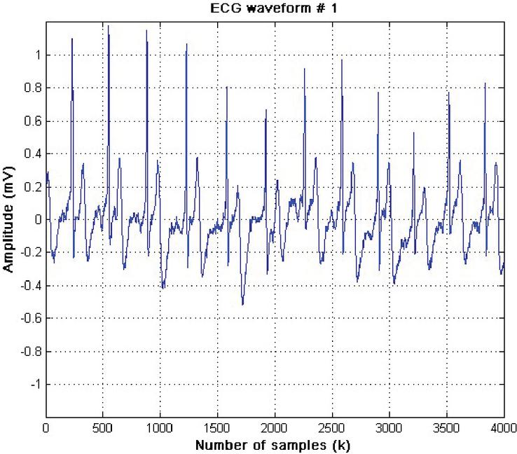
Figure 2 Motion artifacts on ECG input signal from a healthy male standing [18].

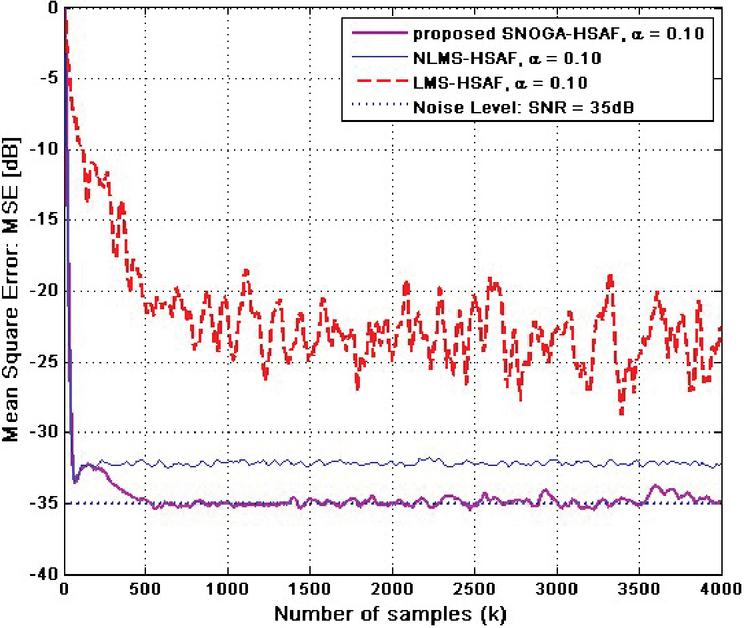
Figure 3 MSE trajectories of SNOGA-HSAF compared with NLMS-HSF [19] and LMS-HSAF [6] using ECG input shown in Figure 2 and $x_n=\alpha \cdot x_{n-1}+\sqrt{1-{\alpha }^2}{\zeta }_n$, where $\alpha =0.10$, ${\mathbf{\text{C}}}_B$ in (62) and SNR $=$ 35 dB.

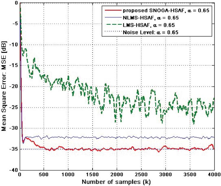
Figure 4 MSE trajectories of SNOGA-HSAF, NLMS-HSF [19] and LMS-HSAF [6] using ECG input shown in Figure 2 and $x_n=\alpha \cdot x_{n-1}+\sqrt{1-{\alpha }^2}{\zeta }_n$, where $\alpha =0.65$, ${\mathbf{\text{C}}}_B$ in (62) and SNR $=$ 35 dB.

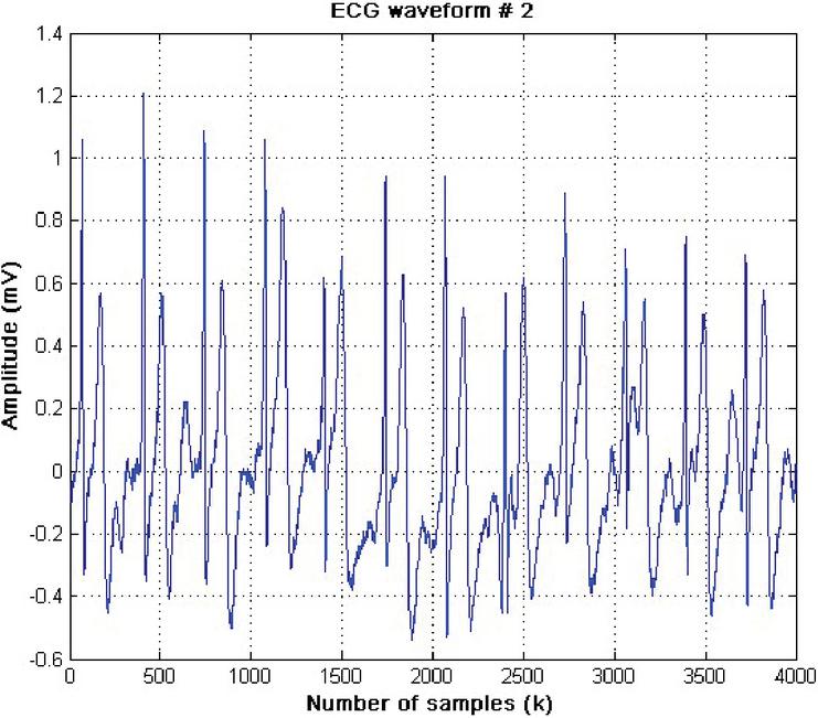
Figure 5 Motion artifacts on ECG input signal from a healthy male walking [18].

Figure 6 MSE trends of SNOGA-HSAF, NLMS-HSF [19] and LMS-HSAF [6] using ECG input shown in Figure 5 and $x_n=\alpha \cdot x_{n-1}+\sqrt{1-{\alpha }^2}{\zeta }_n$, where $\alpha =0.10$, ${\mathbf{\text{C}}}_B$ in (62) and SNR $=$ 35 dB.

Figure 7 MSE trends of SNOGA-HSAF, NLMS-HSF [19] and LMS-HSAF [6] using ECG input shown in Figure 5 and $x_n=\alpha \cdot x_{n-1}+\sqrt{1-{\alpha }^2}{\zeta }_n$, where $\alpha =0.65$, ${\mathbf{\text{C}}}_B$ in (62) and SNR $=$ 35 dB.

The initial parameters for HSAF model of adaptive linear FIR filter are as ${\delta }_w=1\times {10}^{-3}$ and the length of coefficients M is equal to 7 taps. Other the initial parameters of proposed SNOGA-HSAF algorithm are used as follows: ${\mu }_w=1.35\times {10}^{-3}$, ${\mu }_q=1.25\times {10}^{-3}$, ${\lambda }_w(0)={\lambda }_q(0)=1.25\times {10}^{-4}$.

For the first experiment, the ECG contaminated input signal performing when standing is shown in Figure 2. MSE learning curves are presented with the different values of $\alpha =0.10,0.65$ and SNR $=$ 35 dB. Figures 3 and 4 depict the MSE curves of SNOGA-HSAF, NLMS-HSAF and LMS-HSAF at $\alpha =0.10,0.65$. It is seen that the MSE trajectories of proposed SNOGA-HSAF and NLMS-HSAF algorithms are close quickly to the steady-state, while the proposed SNOGA-HSAF algorithm can converge rapidly in comparison with conventional LMS-HSAF algorithm.

For the second experiment, the ECG contaminated input signal performing when walking is shown in Figure 5. And Figures 6 and 7 depict the MSE learning curves of proposed SNOGA-HSAF, NLMS-HSAF and LMS-HSAF at $\alpha =0.10,0.65$. It is confirmed that the MSE curves of proposed SNOGA-HSAF and NLMS-HSAF algorithms are close quickly to the steady-state, while the proposed SNOGA-HSAF algorithm can converge rapidly compared with conventional LMS-HSAF algorithm.

5 Conclusion

A proposed spline-based Hammerstein adaptive filtering on the sign normalised orthogonal gradient adaptive algorithm (SNOGA-HSAF) has been proposed. The proposed SNOGA algorithm has been described how to derive on the spline-based Hammerstein adaptive filtering. Minimum mean square error is used as a measurement model. The proposed SNOGA-HSAF algorithm has been investigated using the MMSE criterion. Performance analysis of proposed SNOGA-HSAF algorithm has been proven in the form of the excess mean square error. Simulation experiments are used the motion artifact ECG input signal recorded when standing and walking. Experimental results perform that the proposed SNOGA algorithm exceeds consistently the standard LMS and NLMS algorithms based on HSAF approach.

Our research will enhance the conventional adaptive filters for the real-time dynamic system. Hammerstein model is being interested in the adaptive signal processing and data analysis. This study is also expected to be useful in adaptive filtering for smart application.

References

[1] S. Kalluri, G.R. Arce. General Class of Nonlinear Normalized Adaptive Filtering Algorithms. IEEE Transactions on Signal Processing, 48(8): 2262–2272, 1999.

[2] M. Scarpiniti, D. Comminiello, R. Parisi and A. Uncini. Nonlinear Spline Adaptive Filtering. Signal Processing, 93(4): 772–783, 2013.

[3] M. Scarpiniti, D. Comminiello, R. Parisi and A. Uncini. Spline Adaptive Filters: Theory and Applications, Adaptive Learning Methods for Nonlinear System Modeling, ELSEVIER, 47–69, 2018.

[4] S. Guan and Z. Li. Normalised Spline Adaptive Filtering Algorithm for Nonlinear System Identification. Neural Processing Letter, 46(2), 595–607, 2017.

[5] M. Scarpiniti, D. Comminiello and A. Uncini. Convex Combination of Spline Adaptive Filters. In Proceedings of IEEE European Signal Processing Conference (EUSIPCO), 2019.

[6] M. Scarpiniti, D. Comminiello, R. Parisi and A. Uncini. Nonlinear System Identification using IIR Spline Adaptive Filters. Signal Processing, 108, 30–35, 2015.

[7] M. Scarpiniti, D. Comminiello, R. Parisi and A. Uncini. Novel Cascade Spline Architectures for the Identification of Nonlinear Systems. IEEE Transactions on Circuits and systems-I: Regular Papers, 62(7), 1825–1835, July 2015.

[8] C. Liu and Z. Zhang. Set-membership Normalised Least M-estimate Spline Adaptive Filtering Algorithm in Impulsive Noise. Electronics Letters, 54(6), 393–395, 2018.

[9] S. Sitjongsataporn and T. Wiangtong. Spline Adaptive Filtering based on Normalised Orthogonal Gradient Adaptive Algorithm. In Proceedings of IEEE International Conference on Engineering, Applied Sciences and Technology (ICEAST), pp. 575–578, 2019.

[10] S. Guarnieri, F. Piazza and A. Uncini. Multilayer Feedforward Networks with Adaptive Spline Activation Function. IEEE Transactions on Neural Network, 10(3): 672–683, 1999.

[11] M. Scarpiniti, D. Comminiello, R. Parisi and A. Uncini. Hammerstein Uniform Cubic Spline Adaptive Filtering: Learning and Convergence Properties. Signal Processing, 100: 112–123, 2014.

[12] P. P. Campo, D. Korpi, L. Anttila and M. Valkama. Nonlinear Digital Cancellation in Full-duplex Devices using Spline-based Hammerstein Model. In Proceedings of IEEE Globecom Workshops (GC Wkshps), 2018.

[13] S. Prongnuch and S. Sitjongsataporn. Stability and Steady-State Performance of Hammerstein Spline Adaptive Filter Based on Stochastic Gradient Algorithm. International Journal of Intelligent Engineering and Systems (IJIES), 13(3), 112–123, 2020.

[14] P.S.R. Diniz. Adaptive Filtering: Algorithms and Practical Implementation. Springer, 2008.

[15] S. Sitjongsataporn. Convergence Analysis of Greedy Normalised Orthogonal Gradient Adaptive Algorithm. In Proceedings of IEEE International Symposium on Communications and Information Technologies (ISCIT), Bangkok, Thailand, pp. 345–348, 2018.

[16] A. L. Goldberger, L. Amaral, L Glass, J. M. Hausdorff, P. Ivanov, R. Mark, J. Mietus, G. Moody, C. Peng, H. Stanley. PhysioBank, PhysioToolkit, and PhysioNet: Components of a New Research Resource for Complex Physiologic Signals. Circulation, 101(23): e215–e220, 2000.

[17] V. Behravan, N. E. Glover, R. Farry, M. Shoaib, P. Y. Chiang. Rate-Adaptive Compressed-Sensing and Sparsity Variance of Biomedical Signals. In Proceedings of IEEE International Conference on Wearable and Implantable Body Sensor Networks (BSN), 2015.

[18] PhysioBank ATM. Retrieved from https://archive.physionet.org/cgi-bin/atm/ATM [Online]. Access on March 22, 2021.

[19] S. Prongnuch, S. Sitjongsataporn, T. Wiangtong. Hammerstein Spline Adaptive Filtering based on Normalised Least Mean Square Algorithm. In Proceedings of IEEE International Symposium on Intelligent Signal Processing and Communication Systems (ISPACS), Taipei, Taiwan, 2019.

Biographies

Suchada Sitjongsataporn received the B.Eng. (First-class honours) and D.Eng. degrees in Electronic Engineering from Mahanakorn University of Technology, Bangkok, Thailand in 2002 and 2009. She has worked as lecturer at department of Electronic Engineering, Mahanakorn University of Technology since 2002. Currently, she is an Associate Professor and the Associate Dean for Research at Faculty of Engineering and Technology in Mahanakorn University of Technology. Her research interests are mathematical and statistical models in the area of adaptive signal processing for communications, networking, embedded system, image and video processing.

Sethakarn Prongnuch received his B.Eng. degree in computer engineering from the Rajamangala University of Technology Phra Nakhon in Bangkok, Thailand in 2011, and the M.Eng. and D.Eng. degrees in Computer Engineering from the Mahanakorn University of Technology in Bangkok, Thailand in 2013 and 2019, respectively. He has worked as a lecturer at the department of Robotics Engineering at Faculty of Industrial Technology in Suan Sunandha Rajabhat University in Bangkok, Thailand since 2013. His research interests include computer architectures and systems, embedded system, and heterogeneous system architecture.

Journal of Mobile Multimedia, Vol. 18_4, 1211–1230.
doi: 10.13052/jmm1550-4646.18412
© 2022 River Publishers

Abstract

1 Introduction

2 Proposed Spline-based Hammerstein Algorithm and System Model

2.1 Spline Interpolation

2.2 Spline-based Hammerstein Model

2.3 Proposed Orthogonal Gradient Sign Algorithm for Spline-based Hammerstein Adaptive Filtering

3 Convergence Properties

3.1 Stability

3.2 Mean Square Analysis

4 Experiment and Simulation Results

5 Conclusion

References

Biographies