Managing Carbon Foot Prints in Supply Chain for Imperfect Quality Items

Sahil Bhardwaj¹, Mandeep Mittal^2,* and Riju Chaudhary¹

¹Department of Mathematics, Amity Institute of Applied Sciences, Amity University Uttar Pradesh, Noida, Uttar Pradesh – 201303, India
²School of Computer Science Engineering and Technology (SCSET), Bennett University, Greater Noida, Uttar Pradesh, India
E-mail: mittal_mandeep@yahoo.com
*Corresponding Author

Received 02 February 2023; Accepted 07 May 2023; Publication 13 September 2023

Abstract

Producing 100% high-quality items is a challenging task in today’s era, which often results in the delivery of defective products. Therefore, inspecting the lot becomes a necessity. This paper investigates the impact of environmental concerns on the inventory model by incorporating fuel costs and emission taxes. The objective of the study is to minimize the expected total cost and determine the optimal order quantity. The study includes a numerical example with sensitivity analysis to determine the model’s robustness. The findings of the study indicate that minimizing emissions also reduces the expected total cost. The paper highlights the significance of considering environmental concerns in inventory management. The study highlights the importance of addressing environmental issues in inventory management and provides a framework for minimizing costs while considering the impact on the environment.

Keywords: EOQ, inspection, imperfect quality items, carbon emission.

1 Introduction

Inventory is the complete list of items which includes the raw materials, semi finished goods in the process of production, and finished goods meant for sale. Inventory management is widely used both in public as well as private sector organizations. The first classic inventory model was developed by Harris (1913) which was known as the EOQ (Economic-Order-Quantity) model. Since then, this subject has drawn the attention of many researchers. According to Hill’s (1997) proposed technique, the shipment must be supplied to the retailer throughout the manufacturer cycle’s production phase.

The restrictions of the EOQ model have been the subject of numerous investigations. One of them is the notion that every item received is flawless. Many academicians have been interested in using inventory models that take into account products of variable quality. The concept of existence of defective items in a lot, and inspection of the lot for probable defects in it, was presented by (Jaggi et al., 2011).

Organizations all over the world are facing a global challenge and issues related to green supply chains and emission reduction. Sustainable practices are being included by businesses in an effort to enhance their strategies and production schedules. Due to concerns about sustainability, the goal is now to both reduce the negative environmental impact and minimise costs. As a result, the notion to include carbon emissions in integrated production models was born. Wahab et al. (2011) took into account an EOQ model with items of variable quality and costs associated with carbon emissions in both the domestic and global supply chains.

Various emission regulation strategies have been used in recent years to limit the emissions produced by supply chain activities. In their study of vendor-buyer cooperative supply chains, Jaber et al. (2013) assumed that the production process was the primary source of emissions and that carbon tax legislation was used to cut those emissions.

Carbon emission during manufacturing process was considered in the models presented by Jaber et al. (2013) and Gurtu et al. (2015). They included transportation cost & carbon emission cost (during transportation of goods) in their proposed models. Hill’s model was further extended and both, transportation cost as well as carbon emission cost during the manufacturing process, were included in the proposed model, by Aljazzar et al. (2017). Yadav et al. (2018) presented cooperative and non co-operative seller–buyer EOQ models with imperfect items, and concluded that the demand function relies on both, the marketing expenditure as well as the selling price of the buyer, stating that the selling price and marketing expenditure of buyer are lower, but order quantity and demand are high in co-operative games as compared to the non-cooperative ones.

Tiwari et al. (2018) looked at a single vendor-buyer supply chain for items that were deteriorating and of poor quality. In their model, they considered the emission of carbon during transporting, storing and holding goods. The fuel used for transportation and the distance travelled, both, affect transportation emissions. Total inventory and energy use per item in the warehouse are also factors that affect carbon emission.

Panuwat Pimsap and Wuttichai Srisodaphol (2022) proposed an Economic Order Quantity (EOQ) model for imperfect items in a lot of products. Their model considered a single sampling plan where a sample from the lot is chosen and inspected by attribute. The acceptance of the order lot is based on the number of defective items in the sample, which should be less than or equal to the acceptance number. If the order lot is rejected, the items in the lot are fully inspected, and the defective items are sent for repair.

S. Singh and R. Chaudhary (2022) presented model for inventory management of perishable items based on expiration dates provides a sustainable approach to managing inventory while minimizing losses, reducing environmental impact, and achieving economic goals.

Naeem et al. (2023) focused on developing a green EOQ inventory model for retailers who receive and store greening items from the seller. Their model consisted of the impact of various factors, such as carbon emissions, greening degree, learning effect, inflationary conditions, and credit financing on the retailer’s total inventory cost. Their aim was to improve the quality of greening items while minimizing the environmental impact and cost for retailers.

Chaudhary et al. (2023) incorporated the concept of carbon emission from warehouse electricity in an EOQ Model with imperfect items and triangular fuzzy demand.

In the current paper, the total cost includes the set-up cost, holding cost, transportation cost, production cost, interest earning and cost of carbon emission during the manufacturing process as well as transportation of items from the vendor to the buyer. The impact of imperfect quality items in the lot on the total cost has been studied.

2 Research Gap

Literature mentioned in the above literature review, comprising of EOQ models with imperfect items and carbon emission, was studied. The contribution of several authors, so far, has been mentioned in Table 1.

Table 1 Contribution table

Author	EOQ Model	Imperfect Items	Carbon Emission
Bazan et al. (2015)	$\mathrm{✓}$		$\mathrm{✓}$
Aljazzar et al. (2016)	$\mathrm{✓}$		$\mathrm{✓}$
Yadav et al. (2018)	$\mathrm{✓}$		$\mathrm{✓}$
Jayaswal et al. (2019)	$\mathrm{✓}$	$\mathrm{✓}$
Jayaswal et al. (2019)		$\mathrm{✓}$
Sarkar et al. (2022)	$\mathrm{✓}$	$\mathrm{✓}$
Yadav et al. (2022)	$\mathrm{✓}$	$\mathrm{✓}$
Pimsap, P., and Srisodaphol, W. (2022)	$\mathrm{✓}$	$\mathrm{✓}$
Singh, S., and Chaudhary, R. (2023)	$\mathrm{✓}$		$\mathrm{✓}$
Naeem Ahmad et al. (2023)	$\mathrm{✓}$		$\mathrm{✓}$
This Paper	$\mathrm{✓}$	$\mathrm{✓}$	$\mathrm{✓}$

3 Notations & Assumptions

The following notations and assumptions are considered to develop the model. The basic assumptions are taken from Hills (1997) and the rest are adopted from the model proposed by Aljazzar et al. (2017).

3.1 Notations

The following notations have been given under below with meaning description

$Q$	$=$	Order lot (decesion variable) (units)
$D$	$=$	Retailer’s demand rate (units/year)
$P$	$=$	Manufacturer’s production rate where $(D<P)$
$A_r$	$=$	Ordering cost for reailer ($/shipment)
$C_r$	$=$	Item unit cost for reailer ($/unit)
$h_r$	$=$	Holding cost for reailer ($/unit/year)
$s_r$	$=$	Storage holding cost for reailer ($/unit/year)
$A_m$	$=$	Ordering cost for manufacturer ($/shipment)
$C_m$	$=$	Item unit cost for manufacturer (in $)
$h_m$	$=$	Holding cost for manufacturer ($/unit/year)
$s_m$	$=$	Storage holding cost for reailer ($/unit/year)
$\lambda$	$=$	Shipment lot size multiplier in a vendor cycle
$T_m$	$=$	Manufacturer’s cycle time $=$ $\lambda$Q/D (year)
$\delta$	$=$	Percentage of defective items
T${}_{\mathrm{e}}$	$=$	Transport emission tax (in $)
T${}_{\mathrm{ci}}$	$=$	Emission tax rate ($/Ton)
$T_{cap}$	$=$	Truck capacity (in integer)
$\eta$	$=$	Number of trucks per shipment (Q/T${}_{\mathrm{cap}}$)
$E_m$	$=$	Manufacturing emission (g/unit)
$d$	$=$	Distance traveled in one side (Km)
${\mathit{TAC}}_R$	$=$	Retailer’s total annual cost (in $)
${\mathit{TAC}}_m$	$=$	Manufacturer’s total annual cost (in $)
$\mathrm{\Psi }$(Q)	$=$	Integrated total annual cost for the supply chain system (in $)

3.2 Assumptions

a. The rate of demand is fixed over horizon time plane, (i.e.) quantity of goods that consumers want to purchase remains the same regardless of changes in other factors such as price, income, or market conditions.

b. Shortages are not permitted in this model – shortages are not permitted as the quantity of goods produced and supplied is equal to the quantity of goods demanded by consumers at all times. This can be achieved through proper production planning, inventory management, and efficient supply chain management.

c. The rate of demand is less than the rate of production – means that businesses are producing more goods than consumers are willing to buy at the current market price. This can result in a surplus of goods, where the quantity supplied exceeds the quantity demanded. It also means that businesses are producing more goods than consumers are willing to buy at the current market price. This can result in a surplus of goods, where the quantity supplied exceeds the quantity demanded.

d. The capacity of all trucks is same and uses same path for each truck during supply chain – Using the same path and capacity for all trucks can simplify logistics and reduce variability, leading to a more efficient and predictable supply chain. However, it can also limit adaptability and make it difficult to respond to unexpected changes or disruptions. This approach may be suitable for simple and stable supply chains, but more complex ones may require more flexibility.

e. Single type of items is used during this supply chain – If a single type of item is used throughout the supply chain, it can simplify the logistics and reduce the complexity of managing inventory, transportation, and other aspects of the supply chain. This is because there is only one type of product to track and manage, which can reduce the likelihood of errors and miscommunications.

f. The cost of holding units is included during non production phase – cost of holding units is typically included during non-production phases such as storage, transportation, or inventory management, as these activities involve holding products or materials for a certain period of time before they are used or sold.

g. Delivered lot has some defective items as it is not possible to do 100% good production. Production of lots may have some defective items in it so impact of this must needs to be observed.

h. Imperfect quality items are sold at low price in another market – after receiving the imperfect items retailer must check it because consumers will not buy defective item but later on after sorting defective items, retailer must try to sell them out in another market as return of defective items is not allowed.

i. Manufacturer emission cost will be fixed during supply chain – manufacturer’s emission cost during the supply chain may not necessarily be fixed. The amount of emissions generated during production and transportation can vary depending on a range of factors, such as the type and efficiency of the production process, the distance and mode of transportation, and the source of energy used.

j. The cost related to holding units is termed as financial cost which will be same during supply chain.

k. The financial cost for retailer is greater than the financial cost of manufacturer at the retailer’s end as manufacturer will get its complete cost after production but retailers has to invest at certain points like holding cost, setup cost, item cost also retailer has to bear cost of imperfect items also if it is not sold at good price.

4 Proposed Model

Our proposed model follows the model mythology of Hill (1997) and its inventory representation has been depicted in Figure 1. Manufacturer prepared Q units as per demanded retailer.

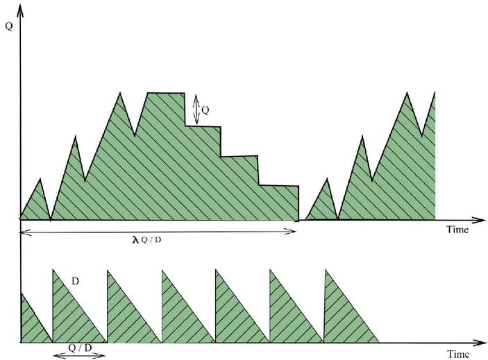
Figure 1 The process of inventory system.

It is supposed that $D$ is the rate of demand for retailer. In this order, we studied the model of Jaber et al. (2013) which presented for the manufacturer emissions which are equal to $E_m=a{P}^2-bP+c$. Gurtu et al. (2015) explained the carbon emission cost associated with transportation and transport with the help of formula (2d eT${}_{\mathrm{ci}}$).

4.1 Retailer’s Total Annual Cost

In this section, we have calculated the total annual cost for the retailer which is the sum of the setup cost SC, item cost IC, holding cost HC, transportation cost TC, and emission tax ET.

Setup cost (SC) encompasses all expenses associated with initiating an order for inventory, which can include costs related to packaging, delivery, shipping, and handling and here it is given as:

$$SC=\left(\frac{(A_r)D}{Q}\right)$$

(1)

Item cost (IC) is the amount paid for the item and any additional direct costs for bringing the item to the facility are included in the item costs of a purchased item & here it is given as:

$$IC=(C_{r}D)$$

(2)

Holding Cost (HC) is the costs associated with keeping inventory or commodities in a warehouse. Inventory holding expenses include rent for the facility, security fees, depreciation costs, and insurance here it is given as:

$$HC=\left((h_r+S_r)\left[\frac{(1-\delta )Q}{2}+\frac{\delta Q^2}{17520}\right]\right)$$

(3)

Transportation cost (TC) is the total cost of transportation includes all expenses that has been associated with moving workers, finished goods, and raw materials. Making ensuring that all moving components are in the right place at the right time to ensure that your consumers receive their goods or services on schedule costs money here it has been given as:

$$TC=\left(\frac{\eta D{A}_0}{Q}+\frac{\eta A_1(2\lambda n-\lambda -1)}{2}\right)$$

(4)

Emission Tax (ET) is the amount of charge or fee paid for every tonne of greenhouse gas emitted. $T_e$, the transportation emission tax, incorporated in this article, was first given by Gurtu et al., (2015). ET has been calculated as:

$$ET=\left(\frac{\eta D{T}_e}{Q}\right)$$

(5)

The Retailer’s annual cost $({\mathit{TAC}}_R)$ can be defined as given below:

${\mathit{TAC}}_R$	$=\mathit{SC}+\mathit{IC}+\mathit{IHC}+\mathit{TC}+\mathit{ET}$	(6)
${\mathit{TAC}}_R$	$={\displaystyle \frac{(A_r)D}{Q}}+C_{r}D+(h_r+S_r)\left[{\displaystyle \frac{(1-\delta )Q}{2}}+{\displaystyle \frac{\delta Q^2}{17520}}\right]$
	$\mathrm{\hspace{1em}}+{\displaystyle \frac{\eta D{A}_0}{Q}}+{\displaystyle \frac{\eta A_1(2\lambda n-\lambda -1)}{2}}+{\displaystyle \frac{\eta D{T}_e}{Q}}$	(7)

4.2 Manufacturer’s Total Annual Cost

In this section, we calculate the total annual cost for the retailer, which is the sum of the setup cost ${\mathit{SC}}_m$, item cost ${\mathit{IC}}_m$, holding cost ${\mathit{IHC}}_m$, transportation cost ${\mathit{TC}}_m$ and emission tax ${\mathit{ET}}_m$.

Setup cost for manufacturer (${\mathit{SC}}_m$) is the cost associated with manufacturer for setup & here it is given as:

$$\left({\mathit{SC}}_m=\frac{(A_m)D}{\lambda Q}\right)$$

(8)

Item cost for manufacturer (${\mathit{IC}}_m$) is the item cost that has been associated with manufacturer & here it is given as:

$$(I{C}_m=C_{m}D)$$

(9)

Holding cost for manufacturer (${\mathit{IHC}}_m$) is the holding cost that has been associated with manufacturer & here it is given as:

$$\left({\mathit{IHC}}_m=(h_m+S_m)\frac{Q}{2}\left[\frac{2D}{P}+\frac{\lambda (P-D)}{P}-1\right]\right)$$

(10)

The transportation cost for the manufacturer (${\mathit{TC}}_m$) refers to the cost of transportation that is directly linked to the manufacturer & here it is given as:

$$\left({\mathit{TC}}_m=\frac{\eta {\mathit{DA}}_0}{Q}+\frac{\eta A_1(2\lambda n-\lambda -1)}{2}\right)$$

(11)

Emission tax for manufacturer (${\mathit{ET}}_m$) is the cost that has been associated with manufacturer for emission during manufacturing the goods. $E_m$ is the emission constrain for manufacturer used by Jaber et al., (2013) and its value is given by $E_m=a{P}^2-bP+c$ and here emission tax for manufacturer is given as:

$$({\mathit{ET}}_M=E_{m}D{T}_{ci})$$

(12)

The manufacturer’s annual cost $({\mathit{TAC}}_m)$ can be defined as given below:

${\mathit{TAC}}_m$	$=S{C}_m+I{C}_m+IH{C}_m+T{C}_m+E{T}_m$	(13)
${\mathit{TAC}}_m$	$={\displaystyle \frac{(A_m)D}{\lambda Q}}+C_{m}D+(h_m+S_m){\displaystyle \frac{Q}{2}}\left[{\displaystyle \frac{2D}{P}}+{\displaystyle \frac{\lambda (P-D)}{P}}-1\right]$
	$\mathrm{\hspace{1em}}+{\displaystyle \frac{\eta D{A}_0}{Q}}+{\displaystyle \frac{\eta A_1(2\lambda n-\lambda -1)}{2}}+E_{m}D{T}_{ci}$	(14)

4.3 Integrated Total Annual Cost for Supply Chain System

In this section, we have calculated total joint cost for supply chain which is the sum of retailer’s annual cost and manufacturer’s cost. From the Equations (4.1) and (4.2), we get

$\mathrm{\Psi }(Q)$	$={\displaystyle \frac{(A_m+\lambda A_r)D}{\lambda Q}}+D(C_r+C_m)$
	$\mathrm{\hspace{1em}}+(h_r+S_r)\left[{\displaystyle \frac{(\mathbf{1}-\mathit{\delta })\mathit{Q}}{\mathbf{2}}}+{\displaystyle \frac{\mathit{\delta }{\mathit{Q}}^{\mathbf{2}}}{\mathbf{17520}}}\right]$
	$\mathrm{\hspace{1em}}+{\displaystyle \frac{(h_m+s_m)Q}{2}}\left\{{\displaystyle \frac{2D}{P}}+{\displaystyle \frac{\lambda (P-D)}{P}}-1\right\}$
	$\mathrm{\hspace{1em}}+{\displaystyle \frac{\eta D{A}_0}{Q}}+{\displaystyle \frac{\eta A_1(2\lambda n-\lambda -1)}{2}}+{\displaystyle \frac{\eta D{T}_e}{Q}}+E_{m}D{T}_{ci}$	(15)

Derivative of total cost function with respect to Q is given below:

${\mathrm{\Psi }}^{\prime }(Q)$	$={\displaystyle \frac{-(A_m+\lambda A_r)D}{\lambda Q^2}}+(h_r+S_r)\left[{\displaystyle \frac{(\mathbf{1}-\mathit{\delta })}{\mathbf{2}}}+{\displaystyle \frac{\mathit{\delta }\mathit{Q}}{\mathbf{8760}}}\right]$
	$\mathrm{\hspace{1em}}+{\displaystyle \frac{(h_m+s_m)}{2}}\left\{{\displaystyle \frac{2D}{P}}+{\displaystyle \frac{\lambda (P-D)}{P}}-1\right\}$
	$\mathrm{\hspace{1em}}-{\displaystyle \frac{\eta D{A}_0}{Q^2}}-{\displaystyle \frac{\eta D{T}_e}{Q^2}}$	(16)

The convexity of joint total cost for supply chain has been shown in Figure 2 with the help of Mathematica software. The complete solution procedure is mentioned in the appendix section.

Figure 2 Convexity of joint total cost for supply chain.

5 Numerical Problem

The numerical analysis used in this study majorly relies on data from previously published paper (Aljazzar et al. 2016). Also, fuel consumption and transport emission data were obtained from Gurtu et al. (2015), while manufacturing emission data were collected from Jaber et al. (2013). The values of the input parameters used in the analysis are listed in Table 2.

Table 2 Input parameters

Variable	Value		Variable	Value
D	1000	units/year	T${}_{\mathrm{cap}}$	80
P	3200	units/year	$\mathit{\delta }$	0.02
A${}_{\mathrm{m}}$	$200	per order	T${}_{\mathrm{ci}}$	30
C${}_{\mathrm{m}}$	$15	per unit	T${}_{\mathrm{e}}$	(2)(d)(0.00077344)(30)
h${}_{\mathrm{m}}$	$ 3	per unit/year	a	0.0000003
s${}_{\mathrm{m}}$	$ 9	per unit/year	b	0.0012
k${}_{\mathrm{m}}$	0.001		c	1.4
A${}_{\mathrm{r}}$	$ 30	per order	E${}_m$	$a{P}^2-bP+c$
C${}_{\mathrm{r}}$	$ 20	per unit	$\mathit{\eta }$	3
h${}_{\mathrm{r}}$	$ 4	per unit per year	$Q^{*}$	223 units
s${}_{\mathrm{r}}$	$ 12	per unit per year	$\mathrm{\Psi }$ (Q*)	60517 ($)
k${}_{\mathrm{r}}$	0.002
T	5
D	500
$\mathit{\lambda }$	2

For the calculation, we used Mathematica software for the optimization of order quantity and total integrated cost for supply chain. The optimal order quantity of this proposed model is $Q^{*}=223$ units and the optimal integrated cost with respect to this optimal order quantity is $\mathrm{\Psi }(Q^{*})=60517$ $. The present study is also compared with previous study and has been shown in the Table 3.

Table 3 Comparison of proposed model with traditional model

Model	Imperfect Items	Lot Size	Total Cost
Base Paper	NA	222	60487
	0.00	222	60487
Proposed Model	0.01	222	60535
	0.02	223	60517

Table 4 Impact of percentage of defective items on lot size and joint total cost

Percentage of Defective Items	Lot Size	Total Cost
0.01	222	60535
0.02	223	60517
0.03	224	60499
0.04	224	60482
0.05	225	60464
0.08	227	60409

Table 5 Impact of demand rate and production on lot size and joint total cost

Demand Rate	Production Rate	Lot Size	Total Cost
1000	3200	223	60517
2000	5200	316	275442
3000	6200	387	610369

Table 6 Impact of number of truck on lot size and joint total cost

Number of Truck	Lot Size	Total Cost
2	190	59491
3	223	60517
4	252	61428
5	277	52258

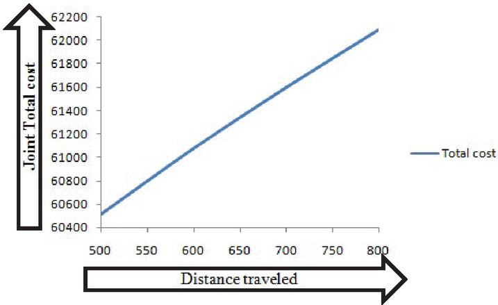
Figure 3 Impact of distance travelled (one side) on total cost.

6 Sensitivity Analysis

Analyzing model parameters is a crucial aspect of research, and sensitivity analysis can help evaluate decisions that are ambiguous. Tables 4, 5, and 6 as well as Figures 3, 4, 5, and 6 provide graphical representations to support this analysis.

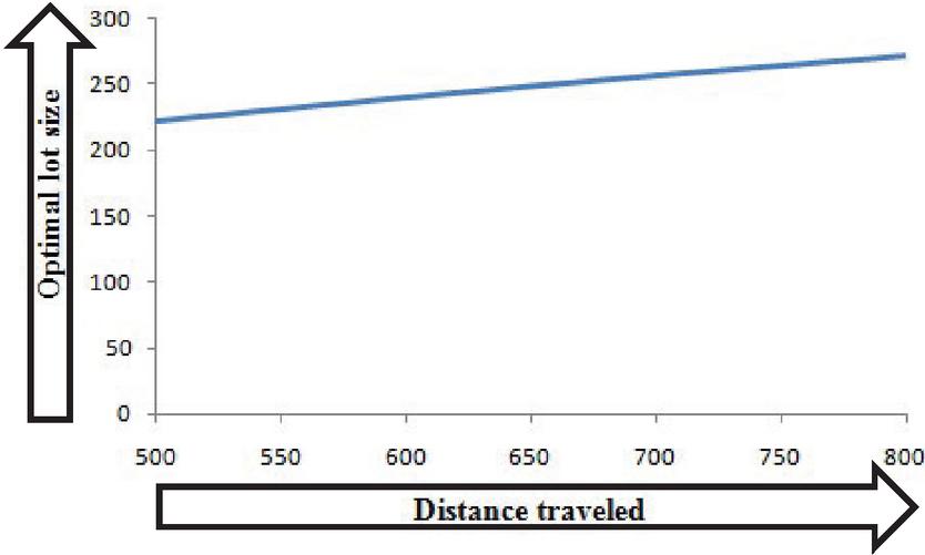
Figure 4 Impact of distance travelled (one side) on order size.

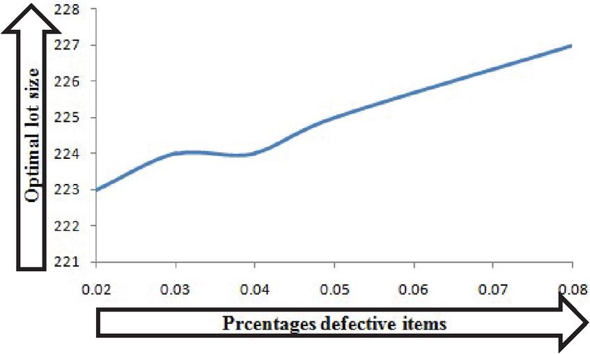
Figure 5 Impact of percentage of defective items on order size.

Figure 6 Impact of percentage of defective items on joint total cost.

6.1 Managerial Insights

a. Table 4 shows that as the percentage of defective items increases, the optimal shipment lot size also increases. However, in such cases, the joint total cost decreases. This observation can assist a manager in making decisions because, despite the increase in the shipment lot size, the total cost is still decreasing.

b. From Table 4, a manager prioritizes managing imperfect items, they can take advantage of this situation. By focusing on reducing the percentage of defective items, the optimal shipment lot size can be increased while also reducing the total cost, resulting in a more efficient and cost-effective supply chain.

c. Analysis of Table 5, Figure 5, and Figure 6 indicates that when there is an increase in demand rate and production rate, the order quantity and joint total cost also increase initially. This observation can assist a manager in understanding the impact of changes in demand and production rates on total cost.

d. By closely monitoring the relationship between demand rate, production rate, order quantity, and joint total cost, a manager can take action to manage the total cost effectively. This may involve adjusting the production rate to meet demand or modifying the order quantity to optimize the joint total cost, resulting in a more efficient and cost-effective supply chain.

e. By analyzing Table 6, it becomes evident that an increase in the number of trucks while keeping other parameters of the model constant results in an increase in the order quantity and joint total cost.

f. From Figures 3 and 4, it can be observed that when distance travelled increases then the total expected total cost increases significantly and it is easier for a one to take decision about delivery of lots keeping distance in mind and hence manager can also imply this to reduce the total cost if distance is reduced so that carbon emission can also be manged with this.

7 Conclusion and Future Scope

The paper aims to investigate the impact of including items with imperfect quality in a lot on various costs and retailer ordering policies. It appears that the paper focuses on the potential advantages of including such items and how it could influence the supply chain. The study suggests that the inclusion of imperfect items can lead to a larger lot size and reduced costs associated with holding, setup, item, transportation, and emission tax. Moreover, the paper highlights the positive impact of carbon emissions and imperfect items on retailer ordering policies.

The paper employs mathematical analysis to support its findings and proposes a model that could be developed with the assistance of a learning and supply chain model under a credit policy. The proposed model is expected to help companies incorporate imperfect items into their supply chain processes in a cost-effective manner.

Overall, the paper highlights the potential benefits of including imperfect items in lot sizes and how this could influence the supply chain. It emphasizes the importance of considering the impact of carbon emissions and imperfect items on retailer ordering policies and how companies can incorporate these factors into their decision-making process. The paper’s findings provide valuable insights for companies looking to optimize their supply chain processes and reduce costs while maintaining quality.

This study provides several opportunities for future research. Firstly, future studies could explore alternative approaches to handling items of defective quality, such as repairing damaged products on-site, hiring staff or purchasing equipment, or sending them to a repair shop instead of selling them at a reduced price. While such alternatives may increase labor, transportation, and repair costs, they may also increase the expected total profit. Additionally, an appropriate extension to the current article would be to consider lead time as a function of production time, setup time, and transportation time. This could provide valuable insights into how lead time affects the total cost and profit of the supply chain. By taking into account these additional factors, future studies can provide more comprehensive recommendations for managers looking to optimize their supply chain operations. Another possible extension could be to allow shortages or partial backlogging, consider learning, and include the concept of trade credit financing.

Appendix

Solution Method

Step 1. Calculate the derivative of cost function $\frac{d\mathrm{\Psi }(Q)}{dQ}=0$.

Step 2. Calculate the second derivative of cost function $\frac{d^2\mathrm{\Psi }(Q)}{d{Q}^2}$.

Step 3. After calculating the second derivative of function it has been observed that it is less than zero $\frac{d^2\mathrm{\Psi }(Q^{*})}{d{Q}^2}<0$, which clearly shows that it is a point of minima.

Step 4. Now solve the equation by using first derivative and put it equal to zero $\frac{d\mathrm{\Psi }(Q)}{dQ}=0$, then we got the minimum value of $(Q)$.

Step 5. With the use of mathematics software the worth of $Q=Q^{*}$ (consider) and calculates $\frac{d^2\mathrm{\Psi }(Q)}{d{Q}^2}$ and if we get $\frac{d^2\mathrm{\Psi }(Q^{*})}{d{Q}^2}<0$, then $Q=Q^{*}$ is called optimal value of $Q$ and denoted by $Q^{*}$.

On differentiating Equation (4.3) with respect to Q and soling it we get

${\mathrm{\Psi }}^{\prime }(Q)$	$={\displaystyle \frac{-(A_m+\lambda A_r)D}{\lambda Q^2}}+(h_r+S_r)\left[{\displaystyle \frac{(\mathbf{1}-\mathit{\delta })}{\mathbf{2}}}+{\displaystyle \frac{\mathit{\delta }\mathit{Q}}{\mathbf{8760}}}\right]$
	$\mathrm{\hspace{1em}}+{\displaystyle \frac{(h_m+s_m)}{2}}\left\{{\displaystyle \frac{2D}{P}}+{\displaystyle \frac{\lambda (P-D)}{P}}-1\right\}-{\displaystyle \frac{\eta D{A}_0}{Q^2}}-{\displaystyle \frac{\eta D{T}_e}{Q^2}}$	(17)
$Q^{*}$	$=\sqrt{{\displaystyle \frac{D*(A_r+\left(\frac{A_m}{\lambda }\right)+\eta *A_0+\eta *T_e}{\begin{array}{c}\left[(h_r+s_r)*\left(\frac{(1-\delta )}{2}+\frac{2*\delta *Q}{175200}\right)\right]\hfill \\ +(h_m+s_m)*\frac{1}{2}*\left(\frac{2*D}{P}+\frac{\lambda *(P-D)}{P}-1\right)\hfill \end{array}}}}$	(18)

References

Ahmad, N., Jaysawal, M. K., Sangal, I., Kumar, S., and Alam, K. (2023, February). Carbon Tax and Inflationary Conditions under Learning Effects: A Green EOQ Inventory Model. In Macromolecular Symposia (Vol. 407, No. 1, p. 2200117).

Aljazzar, S. M., Jaber, M. Y., and Moussawi-Haidar, L. (2016). Coordination of a three-level supply chain (supplier–manufacturer–retailer) with permissible delay in payments. Applied Mathematical Modelling, 40(21–22), 9594–9614.

Bazan, E., Jaber, M. Y., and Zanoni, S. (2015). Supply chain models with greenhouse gases emissions, energy usage and different coordination decisions. Applied Mathematical Modelling, 39(17), 5131–5151.

Chaudhary, R., Mittal, M., and Jayaswal, M. K. (2023). A sustainable inventory model for defective items under fuzzy environment. Decision Analytics Journal, 100207.

Gurtu, A., Jaber, M. Y., and Searcy, C. (2015). Impact of fuel price and emissions on inventory policies. Applied Mathematical Modelling, 39(3–4), 1202–1216

Jaber, M. Y., Glock, C. H., and El Saadany, A. M. (2013). Supply chain coordination with emissions reduction incentives. International Journal of Production Research, 51(1), 69–82.

Jaggi, C. K., and Mittal, M. (2011). Economic order quantity model for deteriorating items with imperfect quality. Investigación Operacional, 32(2), 107–113.

Jayaswal, M., Sangal, I., Mittal, M. and Malik, S. (2019). Effects of learning on retailer ordering policy for imperfect quality items with trade credit financing. Uncertain Supply Chain Management, Vol. 7, No. 1, pp. 49–62.

Jayaswal, M., Sangal, I., Mittal, M. and Malik, S. (2019). Learning effects on stock policies with imperfect quality and deteriorating items under trade credit. Amity International Conference on Artificial Intelligence (AICAI), pp. 499–506. IEEE.

Ibrahim, M. F., Putri, M. M., and Utama, D. M. (2020). A literature review on reducing carbon emission from supply chain system: drivers, barriers, performance indicators, and practices. In IOP Conference Series: Materials Science and Engineering (Vol. 722, No. 1, p. 012034). IOP Publishing.

Parvathi, S., and Raghavan, S. S. (2014). General analysis of single product inventory model–with production by two units system and sales. Journal of Reliability and Statistical Studies, 119–128.

Pimsap, P., and Srisodaphol, W. (2022). Economic order quantity model of imperfect items using single sampling plan for attributes. Journal of Applied Science and Engineering, 25(6), 1217–1225.

Roger, M. (1997). Hill. The single-vendor single-buyer integrated production-inventory model with a generalized policy. European Journal of Operational Research, 97(3), 493–499.

Rout, C., Paul, A., Kumar, R. S., Chakraborty, D., and Goswami, A. (2020). Cooperative sustainable supply chain for deteriorating item and imperfect production under different carbon emission regulations. Journal of Cleaner Production, 272, 122170.

Sarkar, S., Tiwari, S., and Giri, B. C. (2022). Impact of uncertain demand and lead-time reduction on two-echelon supply chain. Annals of Operations Research, 315(2), 2027–2055.

Singh, S., and Chaudhary, R. (2023). Effect of inflation on EOQ model with multivariate demand and partial backlogging and carbon tax policy. Journal of Future Sustainability, 3(1), 35–58.

Srivastava, M., and Gupta, R. (2009). EOQ model for time-deteriorating items using penalty cost. Journal of Reliability and Statistical Studies, 67–76.

Thomas, J. T., and Kumar, M. (2022). Design of fuzzy economic order quantity (EOQ) model in the presence of inspection errors in single sampling plans. Journal of Reliability and Statistical Studies, 211–228.

Tiwari, S., Daryanto, Y., and Wee, H. M. (2018). Sustainable inventory management with deteriorating and imperfect quality items considering carbon emission. Journal of Cleaner Production, 192, 281–292.

Yadav, R., Pareek, S., and Mittal, M. (2018). Supply chain models with imperfect quality items when end demand is sensitive to price and marketing expenditure. RAIRO-Operations Research, 52(3), 725–742.

Yadav, R., Pareek, S., Mittal, M., and Jayaswal, M. K. (2022). Two-level supply chain models with imperfect quality items when demand influences price and marketing promotion. Journal of Management Analytics, 9(4), 480–495.

Biographies

Sahil Bhardwaj is a promising young researcher serving as a Research Scholar at the Department of Mathematics within the Amity Institute of Applied Sciences at Amity University Uttar Pradesh, Noida, India. His research focuses on several areas, notably Inventory Management, Supply Chain Optimization, and Data Envelopment Analysis. Sahil possesses a strong command over various software tools and programming languages, including Mathematica, and Lingo. His expertise and dedication make him a valuable asset in his field of study.

Mandeep Mittal is a seasoned Professor having 23 years’ experience in higher education institutions. Currently, he is working as a Professor in the School of Computer Science Engineering and Technology (SCSET), Bennett University, The Times Group. He earned his post-doctorate from Hanyang University, South Korea, Ph.D. from the University of Delhi, India, and postgraduation from IIT Roorkee, India. He has published more than 100 research articles in the International Journals/book chapters/conferences. He authored one book with Narosa Publication on C language and edited eight research books with IGI Global, USA and Springer, Singapore. He is a series editor of Inventory Optimization, Springer Singapore Pvt. Ltd. He guided 6 Ph.D. scholars, and 6 students are working with him in the area of Inventory Control and Management. He served as Head of the Department of Mathematics and Dean of Students Activities at Amity School of Engineering and Technology. He is a member of the editorial board of international journals. He actively participated as a core member of organizing committees in the international conferences in India and outside India.

Riju Chaudhary is an accomplished academic professional serving as an Assistant Professor and Research Scholar at the Department of Mathematics, Amity Institute of Applied Sciences, located in Amity University Uttar Pradesh, Noida, India. With an impressive teaching and research career spanning over 13 years, Riju’s expertise lies in various research domains, including Inventory Management, Supply Chain Optimization, Fuzzy Theory, and Data Envelopment Analysis, among others.

Riju possesses extensive knowledge of software tools and programming languages, which significantly enhances her research capabilities. She is proficient in utilizing Mathematica, Matlab, C++, and Lingo to facilitate her analytical and computational work. Riju’s proficiency in these tools allows her to explore complex mathematical models, conduct data analysis, and optimize supply chain processes effectively.

Her extensive teaching experience and research background make Riju an invaluable asset to the Department of Mathematics. Her passion for mathematics and dedication to advancing knowledge in her research areas contribute significantly to the academic and research community.

Journal of Reliability and Statistical Studies, Vol. 16, Issue 1 (2023), 117–136.
doi: 10.13052/jrss0974-8024.1616
© 2023 River Publishers

Abstract

1 Introduction

2 Research Gap

3 Notations & Assumptions

3.1 Notations

3.2 Assumptions

4 Proposed Model

4.1 Retailer’s Total Annual Cost

4.2 Manufacturer’s Total Annual Cost

4.3 Integrated Total Annual Cost for Supply Chain System

5 Numerical Problem

6 Sensitivity Analysis

6.1 Managerial Insights

7 Conclusion and Future Scope

Appendix

Solution Method

References

Biographies