Statistical Inference for Multi State Systems under the Generalized Modified Weibull Class

Andreas Makrides

Laboratory of Statistics and Data Analysis, Department of Statistics and Actuarial-Financial Mathematics, University of the Aegean, Greece
E-mail: amakridis@aegean.gr

Received 11 October 2021; Accepted 01 May 2022; Publication 22 July 2022

Abstract

Multi state systems can be seen as semi-Markov processes by considering an arbitrary distribution function for sojourn times. Especially, in this work, the Modified Weibull distribution is employed to be the distribution of sojourn times with a shape parameter $λ$ such that is member of a distributions family that is closed under minima. Parameters estimators are provided and the proposed methodology is evaluated using a detailed simulation procedure.

Keywords: Multi-state system, semi-Markov processes, H-class of distributions, Modified Weibull distribution, parameter estimation.

1 Introduction

There is a great interest in developing generalized families of distributions using a function $G$ corresponding to a classical distribution, as the baseline (parent) distribution for the generalization. Such generalizations are quite popular primarily because some phenomena cannot be satisfactorily described by classical distributions, a defect that can be resolved if additional complexity is introduced into the parent distribution. Indeed, it is not uncommon that the tail and skewed behavior cannot be easily captured which affects the accuracy in terms of both description and prediction. It is the class of such $G$ families of distributions that improves the goodness-of-fit and consequently the overall modelling process.

One of the first such families introduced by [2] is the Gompertz-Verhulst family which itself belongs to the so called exponentiated family and is used among others, for the analysis of the growth curve mortality. Following this first family, several other families were proposed like the skewed family [1], the Marshall-Olkin extended (MOE) family [13], the Beta G family [9], the Gamma generated (GG) family [16] and the exponentiated exponential – Poisson family [15] just to mention a few. In this work we focus on the 4-parameter Modified Weibull Poisson (MWP) distribution [8] for developing a new general H-class of distributions with MWP as the baseline parent distribution.

Consider the Modified Weibull distribution introduced in [10] defined by

g (z) = a z^{γ - 1} (γ + β z) \exp (β z - a z^{γ} e^{β z}), a, γ > 0, β \geq 0

(1)

and

G (z) = 1 - e^{- a z^{γ} e^{β z}}, a, γ > 0, β \geq 0 .

(2)

If $N$ is a random variable with zero-truncated Poisson mass distribution with parameter $λ$ then the conditional distribution of the minimum ordered statistic $X = Z_{(1)}$ of a random sample from (1) given $N$ , is given by

f_{X | N} (x | n) = a n e^{- a n x^{γ} e^{β x}} x^{γ - 1} (γ + β x) e^{β x} .

(3)

Summing over all values of $N$ we obtain the marginal distribution given below

f_{X} (x) = a λ x^{γ - 1} {(1 - e^{- λ})}^{- 1} (γ + β x) e^{β x - a x^{γ} e^{β x} - λ (1 - e^{- a x^{γ} e^{β x}})} .

(4)

The above distribution is known as the Modified Weibull Poisson (MWP) distribution with cumulative distribution function

F (x) = \frac{e^{λ}}{e^{λ} - 1} (1 - e^{- λ (1 - e^{- a x^{γ} e^{β x}})}), x > 0 .

(5)

Under the assumption that the parameter $λ$ is such that the term $\frac{e^{λ}}{e^{λ} - 1} \approx 1$ a general class of distributions with MWP as a baseline distribution can be considered by using a parent continuous distribution function, say $H (\cdot)$ . Hence, based on an arbitrary parent distribution we introduce a family of distributions with Modified Weibull Poisson as the baseline distribution, defined by

F (x; λ) = 1 - e^{- λ (H (x))}, x > 0 .

(6)

where $λ > 0$ is the shape parameter of the proposed class. Note that additional distributional parameters associated with the parent distribution $H (\cdot)$ may also be involved in (6).

The present work concentrates on the family in (6) using a parent continuous distribution function and discuss some of its properties. Parameter estimators for (6) are provided, under a multi state system (see [12]), that are assumed to not be constant over time evolution. Asymptotic results regarding the proposed parameter estimates are also provided. The performance of the proposed methodology is investigated by simulated results.

The manuscript is structured in 6 sections. The second section establishes a family of distributions with the Modified Weibull distribution as the baseline distribution. In the third section we discuss the semi-Markov setting that is used in order to estimate, in Section 4, the parameters involved. The semi-Markov transition matrix, in addition with some reliability indices are established in Section 5. Finally, the accuracy of the proposed methodology is evaluating in Section 6.

2 The H-Class of Distributions

Let us define the general family of distribution functions with shape parameter $λ$ given by

F (t; λ) := 1 - {(1 - F (t; 1))}^{λ}

(7)

which meets the conditions according to the Lebesgue measure, with pdf $f (\cdot; λ)$ . Typical members of the family are classical distributions like the exponential and Weibull. The main feature of the family (7) is that the cdf of the minimum ordered statistic of a random sample $X_{1}, X_{2}, \dots, X_{n}$ from (7) falls into the same family (see [3]; [4]).

Observe that clearly the MWP distribution given in (5) is a member of the class (7). In what follows we introduce a generalized cfamily using an arbitrary function $H (\cdot)$ , with the MWP distribution as the parent (baseline) distribution function, defined in (6).

Observe that the proposed generalized H-class of distributions consists of distributions (each having a different H function) falling within the class (7) and each of which is based on the parent MWP distribution which is also a member of (7).Thus, focusing on a single member of (7) we create a generalized family of distributions by adding extra complexity into the baseline MWP distirbution and at the same time staying within the class (7).

Remark 1 It is remarkable that the exponential distribution is obtained when the function $H (\cdot)$ is the identity.

Observe that the H-class in (6) generates a family of distributions which extends greatly the applicability of the Modified Weibull Poisson distribution covering among others, classical problems in engineering, reliability and safety as well as in any other field where the time-to-event is of primary interest.

2.1 Basic Statistical and Reliability Functions

Assume that $H (\cdot)$ has pdf denoted by $h (\cdot)$ . It is easy to see that the density function of a typical member of the H-class (6) is

f (t) = λ h (t) e^{- λ H (t)},

(8)

where $h (t) = \frac{d H (t)}{d t}$ the pdf associated with $H (\cdot)$ .

Recall that the baseline distribution of the (6) is the MWP distribution given in (5) with parameters $a, λ$ and $β, γ \geq 0$ which is denoted by MWP( $a, β, γ, λ$ ) and it is obtained if in (6) we take $H (t) = 1 - e^{- a t^{γ} e^{β t}}$ .

Taking the Weibull distribution $H (t) = 1 - e^{- a t^{γ}}$ as a parent distribution (i.e. setting $β = 0$ in the baseline distribution), we have the Weibull Poisson distribution

F (t) = 1 - e^{- λ (1 - e^{- a t^{γ}})},

(9)

and

f (t) = a λ e^{- λ (1 - e^{- a t^{γ}})} e^{- a t^{γ}} (γ t^{γ - 1}) .

(10)

Observe that the Exponential Poisson distribution is obtained if $H (t) = 1 - e^{a t}$ i.e. if we take $β = 0$ and $γ = 1$ in the baseline distribution.

As expected, irrespectively of the parent distribution, the resulting distribution is a member of the H-class of distributions given in (6). The result is summarized below:

Proposition 1 For any specific parent continuous distribution $H (\cdot)$ the resulting $F (\cdot)$ creates a new class of distributions like (6).

Proposition 2 Assume that the cdf of the r.v. $T$ falls into the class (6). Then, the reliability function $R (\cdot; λ)$ is equal to

R (t; λ) := {[e^{- H (t)}]}^{λ}

(11)

and the instantaneous failure rate $h_{T}$ defined as

h_{T} (t; λ) = λ h (t) .

(12)

The result is immediate from the definitions of the reliability and hazard functions and the expressions (6) and (8).

2.2 H-class: A Class Closed Under Minima

In this section we establish that the H-class in (6) is closed under minima which is a significant property which plays a key role in the statistical inference of the multi-state setting of the next section. More precisely, the above property is important for establishing the expressions for the quantities of interest of the SMM (see Proposition 3). Although it is not a necessary condition, it provides the ability to obtain a closed form for the expressions of the main characteristics of the proposed model.

Theorem 1 If $X_{1}, \dots, X_{n}$ are i.i.d. r.v’s from (6), then the cdf $F_{m i n}$ of $X_{(1)}$ satisfies the property (7).

For the required cdf we can easily see that

$F_{m i n} (t)$	$=$	$1 - {[1 - P (X_{i} \leq t)]}^{n} = 1 - {[e^{- λ H (t)}]}^{n}$
	$=$	$1 - e^{- n λ H (t)}$

which belongs to H-class in (6) with shape parameter $n λ$ .

For the Weibull distribution which ibelongs to the above family, the cdf of the minimum becomes

F (t) = 1 - e^{- n λ (1 - e^{- a t^{γ}})} .

(13)

Remark 2 The results of this section can be generalized by dropping the assumption of identically distributed random variables. Indeed, if one considers the case of independent random variables which though are not necessarily identically distributed (inid) and assumes a random sample $X_{1}, \dots, X_{n}$ with the cdf of $X_{i}$ , $i = 1, \dots, n$ being given by

F (t; λ_{i}) := 1 - e^{- λ_{i} H (t)}

(14)

then, Theorem 1 still holds with $F_{m i n}$ belonging to the H-class (6) with parameter $\sum_{i = 1}^{n} λ_{i}$ , that is

F (t) = 1 - e^{- \sum_{i = 1}^{n} λ_{i} H (t)} .

(15)

In the following section we focus on the inid case for multi-state systems with $N$ (finite) number of states and sojourn times $T_{i j}$ (the time spend on state $i$ before moving to state $j$ ) having a cdf $F_{i j} (\cdot; λ_{i j})$ belonging to the family (6) with shape parameter $λ_{i j}$ , $i, j \in {1, 2, \dots, N}$ .

3 The Semi-Markov Model – The General Setting

Let the semi-Markov process (SMP) $Z = {(Z_{t})}_{t \in ℝ_{+}}$ where

• $E = {1, \dots, N},$ $N < \infty,$ (cf. [11]) is the state space,

• $S = {(S_{n})}_{n \in ℕ}$ represent the jump times,

• $J = {(J_{n})}_{n \in ℕ}$ are the visited states

• $X = {(X_{n})}_{n \in ℕ}$ are the successive sojourn times with $X_{0} = S_{0} := 0$ and

• $N (t) := \max {n \in ℕ ∣ S_{n} \leq t}, t \in ℝ_{+},$ (16)

is the process that counts the jumps in $(0, t]$ .

Observe that $Z_{t} := J_{N (t)}$ is equivalent to $J_{n} = Z_{S_{n}} .$

It is easily showed that ${(J_{n})}_{n \in ℕ}$ is a Markov chain (MC).

Under the assumption that SMP is ergodic (interested readers are referred to [11]), the main features of the model are the initial law

μ = (μ_{1}, \dots, μ_{N}) where μ_{j} := ℙ (J_{0} = j), j \in E,

and the semi-Markov kernel

Q_{i j} (t) := ℙ (J_{n} = j, X_{n} \leq t | J_{n - 1} = i) .

Define also by

p_{i j} := ℙ (J_{n} = j | J_{n - 1} = i) = lim_{t \to \infty} Q_{i j} (t)

the associated the transition probabilities while the conditional sojourn time distribution functions are given below:

W_{i j} (t)

:=

ℙ (S_{n} - S_{n - 1} \leq t | J_{n - 1} = i, J_{n} = j) .

Let us consider some random variables $T_{i j}$ with c.d.f. $F_{i j} (t; λ_{i j}) .$ A specific system is considered in this work which has the property that the state of the system visited directly after state $i$ is the state for which $T_{i j}$ is minimized. Several remarks need to be done here.

Remark 3

(a) The motivation of the framework that we have just described comes from the fact that one could see these $T_{i j}$ s as potential sojourn times in $i$ before jumping to $j;$ for various reasons (minimum cost, minimum waiting time, first come first served, etc.), there is an interest in choosing the minimum of them.

(b) Note that this framework has been considered also in [4], but for different family of distributions.

(c) This could be an interesting and rich framework for modelling time varying parameters with a similar approach like in [6].

Under this setting, we can write

p_{i j}

=

ℙ (T_{i j} \leq T_{i l}, \forall l | J_{n - 1} = i)

and

W_{i j} (t) = ℙ (\min_{l} T_{i l} \leq t | J_{n - 1} = i) = : W_{i} (t),

which is independent of the state $j$ and represents the unconditional cdf of the sojourn time in state $i$ irrespectively of the state to be visited next. We finally assume that the associated pdf is denoted by $f_{i} (t)$ .

The following Proposition from [5] holds true for the class of distributions (6).

Proposition 3

$Q_{i j} (t) = \frac{λ_{i j}}{\sum_{k \in E} λ_{i k}} [1 - e^{- \sum_{k \in E} λ_{i k} H (t)}],$	(17)
$p_{i j} = \frac{λ_{i j}}{\sum_{k \in E} λ_{i k}},$	(18)
$W_{i} (t) = 1 - e^{- \sum_{j = 1}^{N} λ_{i j} H (t)}$	(19)

and

f_{i} (t) = \sum_{j = 1}^{N} λ_{i j} h (t) [1 - e^{- \sum_{j = 1}^{N} λ_{i j} H (t)}]

(20)

4 The Semi-Markov Model – Estimation with and Without Censoring

We proceed now to statistical inference by focusing on $L$ sample paths, $L = 1, 2, \dots$ , under two different settings: the uncensored case where all sojourn times are observed and the censored case with the sojourn time in the last visited state being right censored with censoring time denoted by $M$ .

Having available a semi-Markov process with $L$ censored sample paths, ${j_{0}^{(l)}, x_{1}^{(l)}, j_{1}^{(l)}, x_{2}^{(l)}, \dots, j_{N^{l} (M)}^{(l)}, u_{M}^{(l)}},$ $l = 1, \dots, L$ and for the family of distribution in (6), the general expression of the likelihood function is given by

$ℒ$	$=$	$(\prod_{i \in E} λ_{i}^{N_{i, 0}^{(L)}}) (\prod_{l = 1}^{L} \prod_{i, j \in E} λ_{i j}^{N_{i j}^{(l)} (M)}) \times$	(21)
		$\times \prod_{l, i, k} [{(1 - F (x_{i}^{(l, k)}))}^{\sum_{j \in E} λ_{i j}} (\frac{f (x_{i}^{(l, k)})}{1 - F (x_{i}^{(l, k)})})] \times$
		$\times (\prod_{i \in E} \prod_{k = 1}^{N_{i, M} (L)} {(1 - F (u_{i}^{(k)}))}^{\sum_{j \in E} λ_{i j}}) .$

where

• $N_{i, 0}^{(L)}$ : number of trajectories beginning from state $i$ ,

• $N_{i}^{(l)} (M)$ : number of visits to state $i$ of the $l^{t h}$ trajectory up to observation time $M$ ,

• $N_{i j}^{(l)} (M)$ : number of transitions from state $i$ to $j$ of the $l^{t h}$ trajectory up to observation time $M$ ,

• $N_{i j} (L, M) := \sum_{l = 1}^{L} N_{i j}^{(l)} (M)$ ,

• $x_{i}^{(l, k)}$ : sojourn time in state $i$ during the $k^{t h}$ visit, $k = 1, \dots, N_{i}^{(l)} (M)$ of the $l^{t h}$ trajectory,

• $u_{M}^{(l)} := M - S_{N^{l} (M)}$ is the $l^{t h}$ trajectory’s observed censored time,

• $N_{i, M} (L) = \sum_{l = 1}^{L} 𝟙_{{J_{N^{l} (M)}^{(l)} = i}}$ is the number of visits in state $i$ , as the last visit, during the $L$ trajectories; it holds that $\sum_{i \in E} N_{i, M} (L) = L;$

• $u_{i}^{(k)}$ : observed censored sojourn time in state $i$ during the $k^{t h}$ visit, $k = 1, \dots, N_{i, M} (L)$ .

The maximization of the likelihood provides the estimator of $λ_{i j}$ which is equal to

{\hat{λ}}_{i j} (L, M) = - \frac{N_{i j} (L, M)}{\sum_{l = 1}^{L} B_{i}^{(l)} (M) + \sum_{k = 1}^{N_{i, M} (L)} \log (1 - F (U_{i}^{(k)}))}

(22)

while the estimator of the initial law by

{\hat{μ}}_{i} (L, M) = \frac{N_{i, 0}^{(L)}}{L} .

(23)

In case of no censoring the sample paths are ${j_{0}^{(l)}, x_{1}^{(l)}$ , $j_{1}^{(l)}$ , $x_{2}^{(l)}$ , $\dots$ , $j_{N^{l} (M)}^{(l)}},$ $l = 1, \dots, L,$ and the associated uncensored likelihood function can be considered as a particular case of the censored likelihoood defined earlier in (21). As a result the expression of the estimator of $λ_{i j}$ in this case, is a simplified version of the one given above for the censored case. Indeed, the resulting estimator is

{\hat{λ}}_{i j} (L, M) = - \frac{N_{i j} (L, M)}{\sum_{l = 1}^{L} B_{i}^{(l)} (M)},

(24)

where

B_{i}^{(l)} (M) = \sum_{k = 1}^{N_{i}^{(l)} (M)} \log (1 - F (X_{i}^{(l, k)})) .

The initial probabilities can be estimated using the following expression

{\hat{μ}}_{i} (L, M) = \frac{N_{i, 0}^{(L)}}{L} .

(25)

Using the proper expression among the previous ones, for the parameter estimates, the following estimators can be easily obtained:

${\hat{p}}_{i j} (M) = \frac{{\hat{λ}}_{i j} (L, M)}{\sum_{l \in E} {\hat{λ}}_{i l} (L, M)} = \frac{N_{i j} (M)}{N_{i} (M)},$	(26)
${\hat{W}}_{i} (t, M) = [1 - e^{- H (t) \sum_{j \in E} {\hat{λ}}_{i j} (L, M)}]$	(27)

and

{\hat{Q}}_{i j} (t, M) = \frac{{\hat{λ}}_{i j} (L, M)}{\sum_{k \in E} {\hat{λ}}_{i k} (L, M)} [1 - e^{- H (t) \sum_{k \in E} {\hat{λ}}_{i k} (L, M)}] .

(28)

4.1 The Case of Modified Weibull Poisson Distribution

It is straithforward that for the uncesored setting, the estimator of the parameter $λ_{i j}$ for MWP, is simplified to

{\hat{λ}}_{i j} (L, M) = \frac{N_{i j} (L, M)}{\sum_{l = 1}^{L} \sum_{k = 1}^{N_{i}^{(l)} (M)} (1 - e^{- a {(x_{i}^{(l, k)})}^{γ} e^{β (x_{i}^{(l, k)})}})} .

(29)

In the censored case the estimator of $λ_{i j}$ becomes

{\hat{λ}}_{i j} (L, M) = \frac{N_{i j} (L, M)}{\begin{matrix} \sum_{l = 1}^{L} \sum_{k = 1}^{N_{i}^{(l)} (M)} (1 - e^{- a {(x_{i}^{(l, k)})}^{γ} e^{β (x_{i}^{(l, k)})}}) \\ + \sum_{k = 1}^{N_{i, M} (L)} (1 - e^{- a {(u_{i}^{(k)})}^{γ} e^{β (u_{i}^{(k)})}}) \end{matrix}} .

(30)

4.2 The Case of the General H-class

Under the censoring setting and for the general case of H-class of distributions, the estimator of the parameter $λ_{i j}$ is

{\hat{λ}}_{i j} (L, M) = \frac{N_{i j} (L, M)}{\sum_{l = 1}^{L} \sum_{k = 1}^{N_{i}^{(l)} (M)} H (X_{i}^{(l, k)}) + \sum_{k = 1}^{N_{i, M} (L)} H (U_{i}^{(k)})} .

(31)

where for $H (\cdot)$ , one can consider any distribution function.

5 Reliability Measures of SMP

The purpose of this section is to remind definitions and results on Markov renewal function, semi-Markov transition probabilities and some reliability measures and to point out how we can estimate these measures. As it will be clear in the sequel, the estimators obtained in the previous section for various cases will furnish corresponding estimators of the reliability measures, Markov renewal function and semi-Markov transition probabilities,.

The Markov renewal function, $Ψ_{i j} (t)$ , $t \geq 0$ , with $i$ and $j$ belonging to the state space $E$ , is given by ([7]; [11])

Ψ_{i j} (t)

=

\sum_{n = 1}^{\infty} Q_{i j}^{(n)} (t),

(32)

where $Q_{i j}^{(n)} (t)$ is the $n^{th}$ convolution of $Q$ .

Since the aforementioned is defined as a function of infinite terms, in practice we use the sum $\sum_{n = 1}^{K} Q_{i j}^{(n)} (t)$ where $K$ is a large enough integer such that $| Q_{i j}^{(K)} (t) - Q_{i j}^{(K - 1)} (t) | < ϵ$ , for a sufficient small $ϵ$ .

For two states $i$ and $j$ , the semi-Markov transition matrix is ([11])

P_{i j} (t) := ℙ (Z_{t} = j | Z_{0} = i) = \int_{0}^{t} Ψ_{i j} (d s) (1 - \sum_{k \in E} Q_{j k}) (t - s) .

Consider now two disjoint subsets of the state space, say $U$ and $D$ corresponding to the up- and down-states the union of which is the entire state space. To simplify matters, let $U = {1, 2, \dots, n - 1, n}$ and $D = {n + 1, n + 2, \dots, N} .$

The reliability function $R (\cdot)$ of the system, evaluated at $t$ is equal to ([14])

R (t) = μ_{U} P_{U U} (t) 1_{n},

where: $P_{U U} (t)$ is the value of $P (t)$ obtained using $Q_{U U} (t),$ the restriction of the kernel $Q (t)$ to the up-states $U;$ $μ_{U}$ is the restriction of the initial distribution $μ$ to the up-states $U;$ $1_{n}$ is a vector of $1$ s.

After obtaining the reliability function, the failure rate can be easily obtained:

r (t) = - \frac{R^{'} (t)}{R (t)}, f o r t > 0 .

Similarly, under the present setting, the availability and maintainability are given by ([14], [11])

$A (t)$	$=$	$μ P (t) 1_{N; n},$	(34)
$M (t)$	$=$	$1 - μ_{D} P_{D D} (t) 1_{N - n},$

where: $1_{N; n} = {(\underset{n}{\underset{⏟}{1, \dots, 1}}, \underset{N - n}{\underset{⏟}{0, \dots, 0}})}^{⊤},$ $1_{N - n}$ is a vector of $1$ s; $P_{D D}$ is the value of $P (t)$ obtained using $Q_{D D} (t),$ the restriction of the kernel $Q (t)$ to the down-states $D;$ $μ_{D}$ is the restriction of the initial distribution $μ$ to the down-states $D .$

The mean time to failure (MTTF) is given by:

M T T F = μ_{U} {(I_{n} - p_{U U})}^{- 1} m_{U},

(35)

where: $m_{U}$ is the restriction to $U$ of the mean sojourn time in state $i$ , $m_{i};$ $p_{U U} (t)$ is the restriction to $U$ of the Markov transition matrix $p .$ A similar expression holds also true for the mean time to repair (MTTR).

Note that, for all $i, j \in E$ , $t \geq 0,$ taken into account the parameter estimates obtained in the previous section for various cases, we can obtain the corresponding plug-in estimators of $Ψ_{i j} (\cdot),$ $P_{i j} (\cdot),$ $R (\cdot),$ $r (\cdot),$ $A (\cdot)$ and $M (\cdot) .$ Finally, $m_{i}$ for any state $i$ , is estimated by

{\hat{m}}_{i}^{(1)} (M) := \int_{0}^{\infty} (1 - {\hat{W}}_{i} (t, M)) d t = \int_{0}^{\infty} (1 - e^{- H (t) \sum_{j = 1}^{N} {\hat{λ}}_{i j} (M)}) d t

{\hat{m}}_{i}^{(2)} (M) := \frac{\sum_{k = 1}^{N_{i} (M)} X_{i}^{(k)}}{N_{i} (M)}

and we can also obtain the plug-in estimator of the MTTF.

6 Simulation Studies

The accuracy of the estimating procedure is examined using simulations in R. A semi-Markov process, with 3 states, for several values of the number of trajectories, $L$ , in both cases of censoring or not, is considered. The sojourn times are taken randomly from a Modified Weibull Poisson distribution with fixed parameters $a = 2, β = 1$ and $γ = 2$ which are chosen arbitrarily:

F_{i j} (t) = 1 - e^{- λ_{i j} (1 - e^{- a t^{γ} e^{β t}})} .

(36)

The total observation time is assumed to be $M = 1000$ and we record the results of the estimated parameters of interest. As for the initial law, is simulated from the discrete Uniform distribution with parameters 1 and $N$ . For the cases where there exist censored paths, using the Uniform distribution, the trajectories with censored sojourn time in the first visited state, are chosen. Randomly we cut the interval that is computed as the first/last sojourn time in two parts, where the second part is considered to be the censored sojourn time in the first/last visited state. Note that modifications of the method described above could be considered.

The two tables below provides the target values of the parameters $λ_{i j}$ and the markov chain transition probabilities $p_{i j}$

{blockarray} c c c c {block} | c | c c c | λ_{i j} & 1 & 2 & 31 & 0 & 5.9 & 4.1 2 & 6.5 & 0 & 4.3 3 & 5.2 & 5.8 & 0 {blockarray} c c c c {block} | c | c c c | p_{i j} & 1 & 2 & 31 & 0 & 0.590 & 0.410 2 & 0.602 & 0 & 0.398 3 & 0.473 & 0.527 & 0

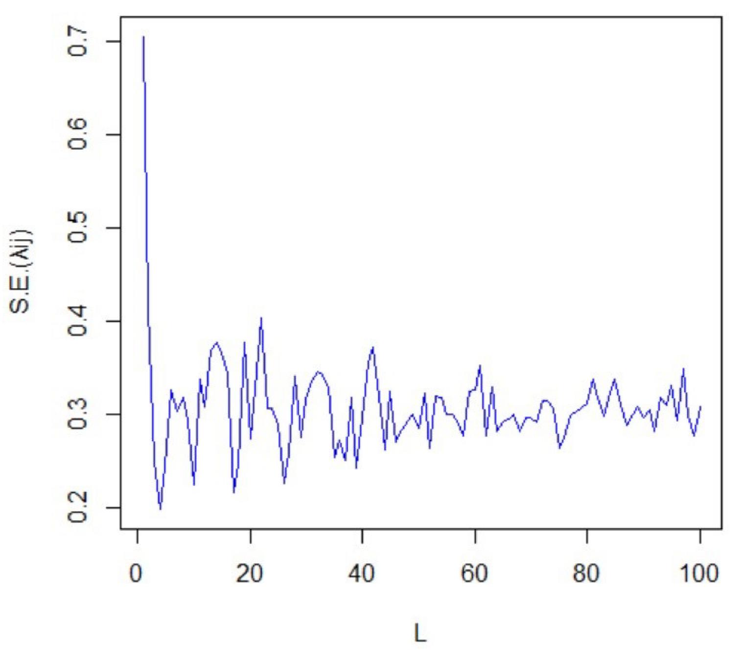
Figure 1 Squared errors of ${\hat{λ}}_{i j}$ for censored trajectories at the beginning and/or at the end, for $L \in [1, 2, \dots, 100]$ .

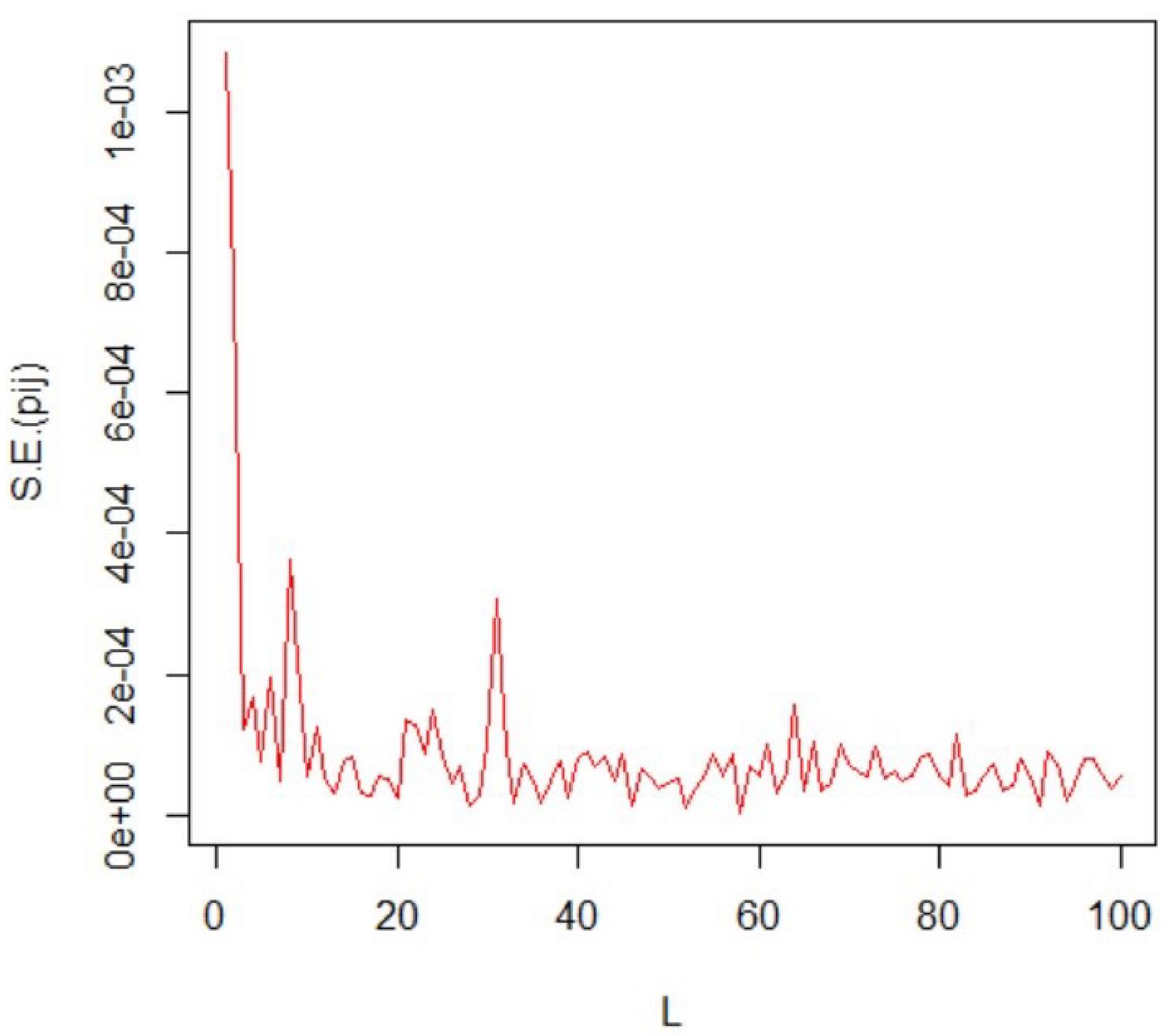
Figure 2 Squared errors of ${\hat{p}}_{i j}$ for censored trajectories at the beginning and/or at the end, for $L \in [1, 2, \dots, 100]$ .

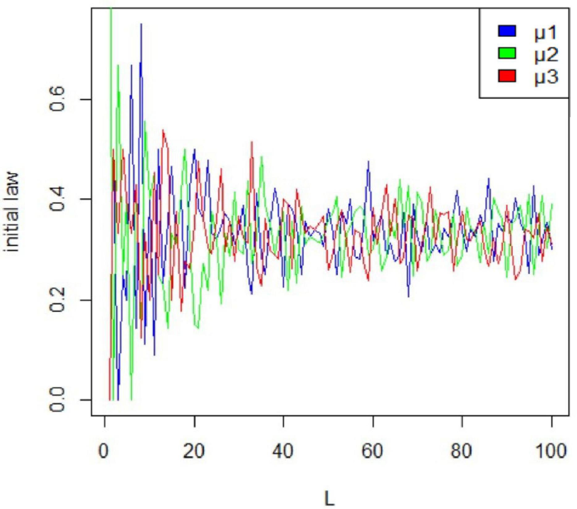
Figure 3 Estimators for the initial law, ${\hat{μ}}_{i}$ for censored trajectories at the beginning and/or at the end, for $L \in [1, 2, \dots, 100]$ .

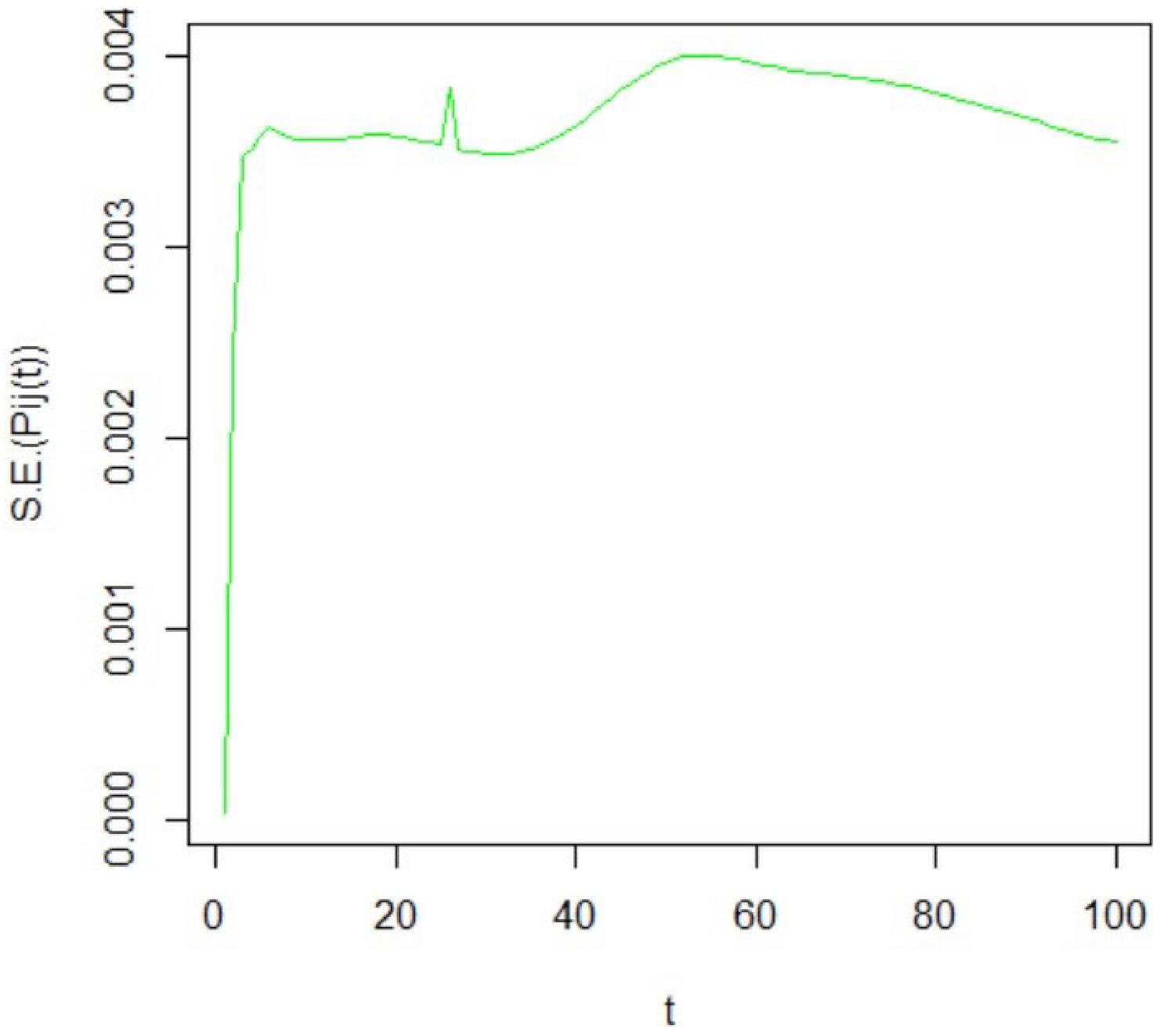
Figure 4 Squared errors of ${\hat{P}}_{i j} (t)$ for censored trajectories at the beginning and/or at the end, for $t \in [1, 2, \dots, 100]$ .

6.1 Censoring at the Beginning and/or at the End

Figures 1 and 2 present the squared errors (S.E.) of the estimators ${\hat{λ}}_{i j}$ and ${\hat{p}}_{i j}$ respectively, as the number of trajectories $L$ increases from 1 to 100. Observe that in almost all cases the estimators of both parameters are very good with respect to the squared errors. However, the squared errors of the markov chain transition probabilities, ${\hat{p}}_{i j}$ , are smaller as compared to the ones of the parameters ${\hat{λ}}_{i j}$ . Figure 3 presents the estimate of the initial law function which is closed to the true value of $(μ_{1}, μ_{2}, μ_{3}) = (\frac{1}{3}, \frac{1}{3}, \frac{1}{3})$

According to Figure 4, the estimated values for the semi-Markov process transition probabilities are very close to the real values with the squared errors to be less than $0.4 %$

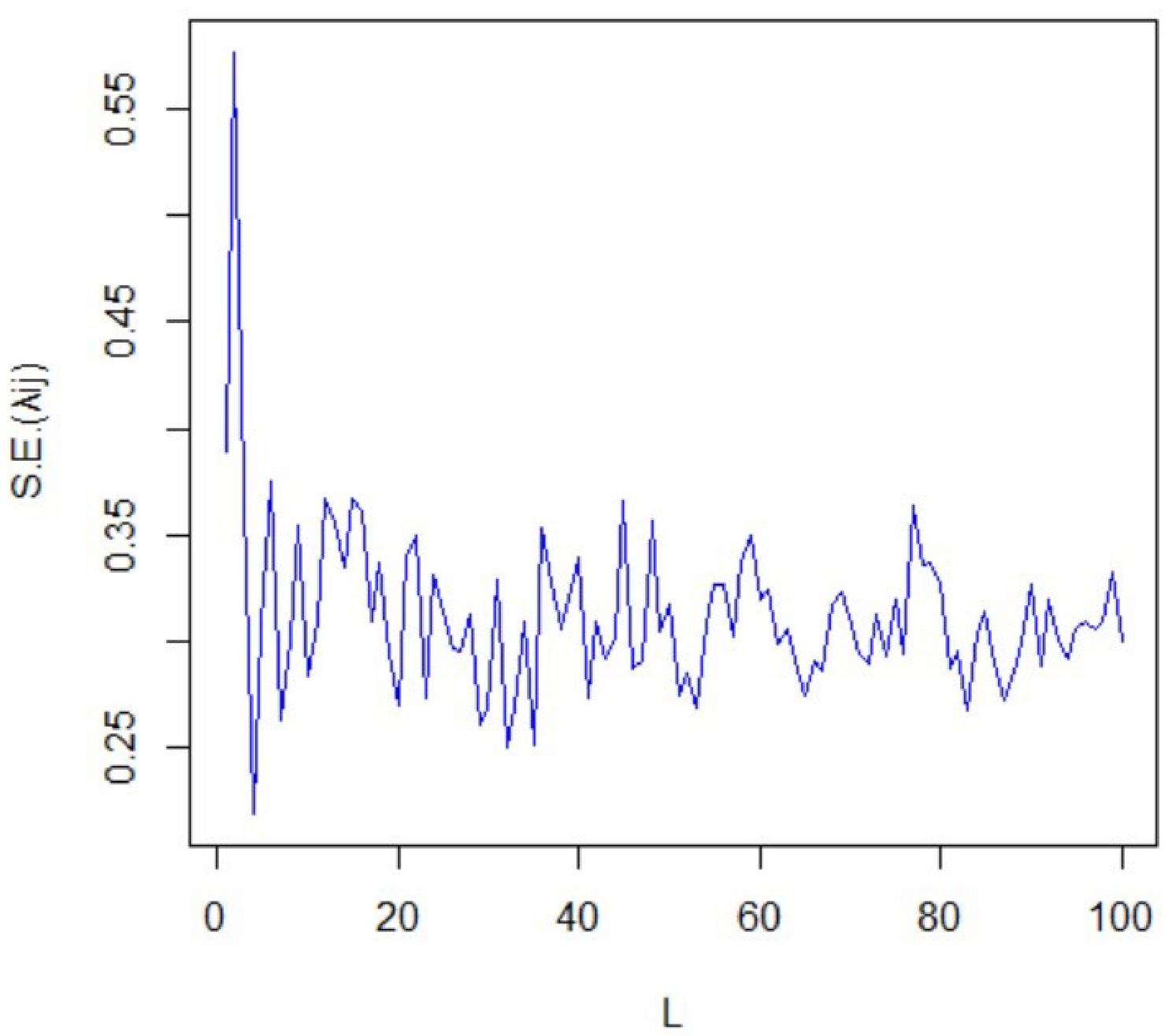
Figure 5 Squared errors of ${\hat{λ}}_{i j}$ for uncensored trajectories, for $L \in [1, 2, \dots, 100]$ .

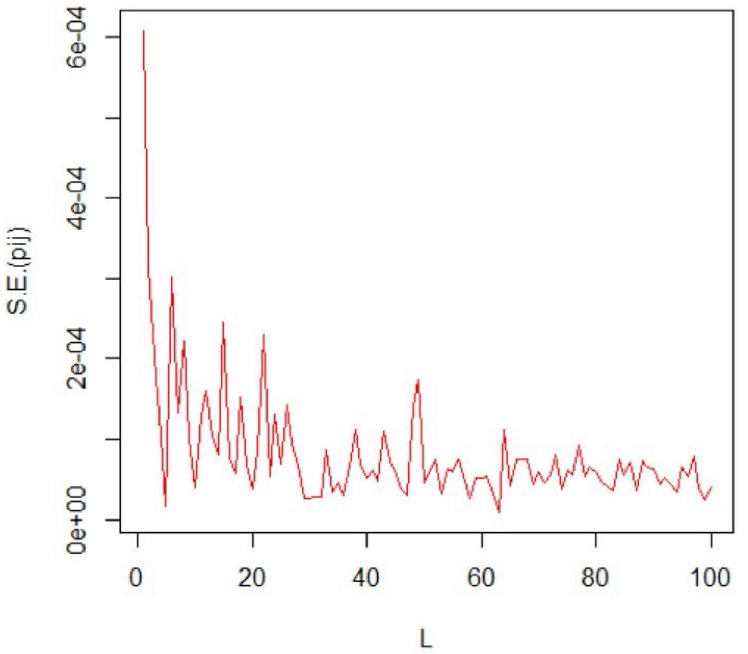
Figure 6 Squared errors of ${\hat{p}}_{i j}$ for uncensored trajectories, $L \in [1, 2, \dots, 100]$ .

6.2 All Samples are Observable Without Censoring

The estimators ${\hat{λ}}_{i j}$ of the parameters for the baseline distribution, MWP, and the markov chain transition probabilities, ${\hat{p}}_{i j}$ , behave very well even in the case of no censoring (see Figures 5 and 6).

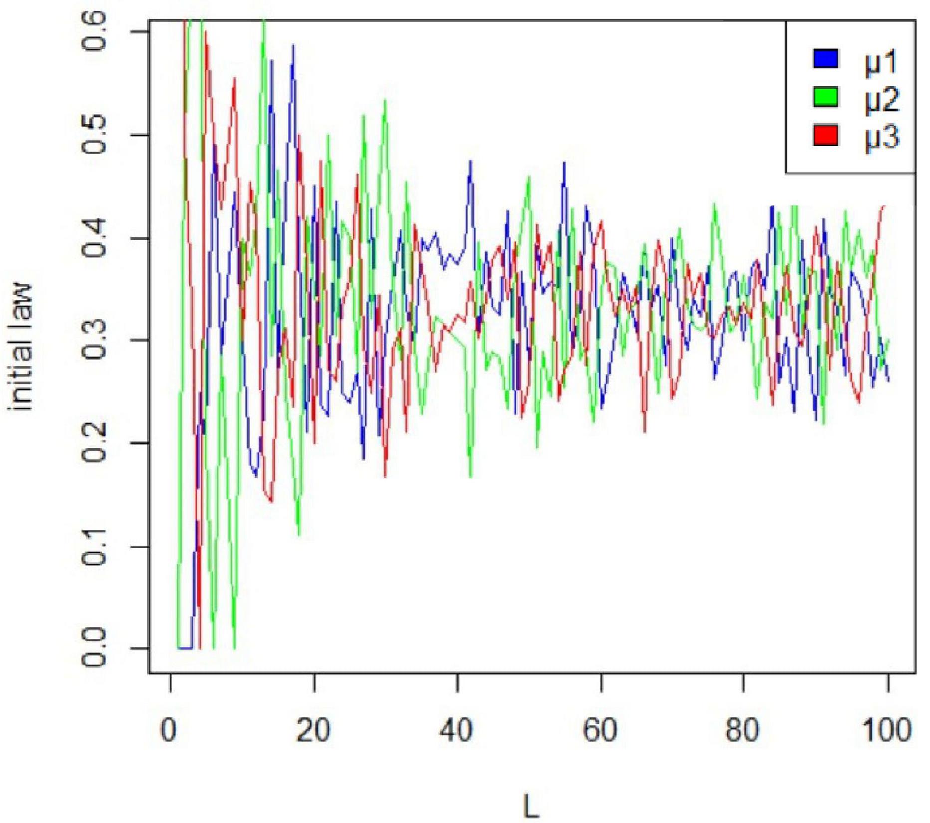
Figure 7 Estimators for the initial law, ${\hat{μ}}_{i}$ for uncensored trajectories, $L \in [1, 2, \dots, 100]$ .

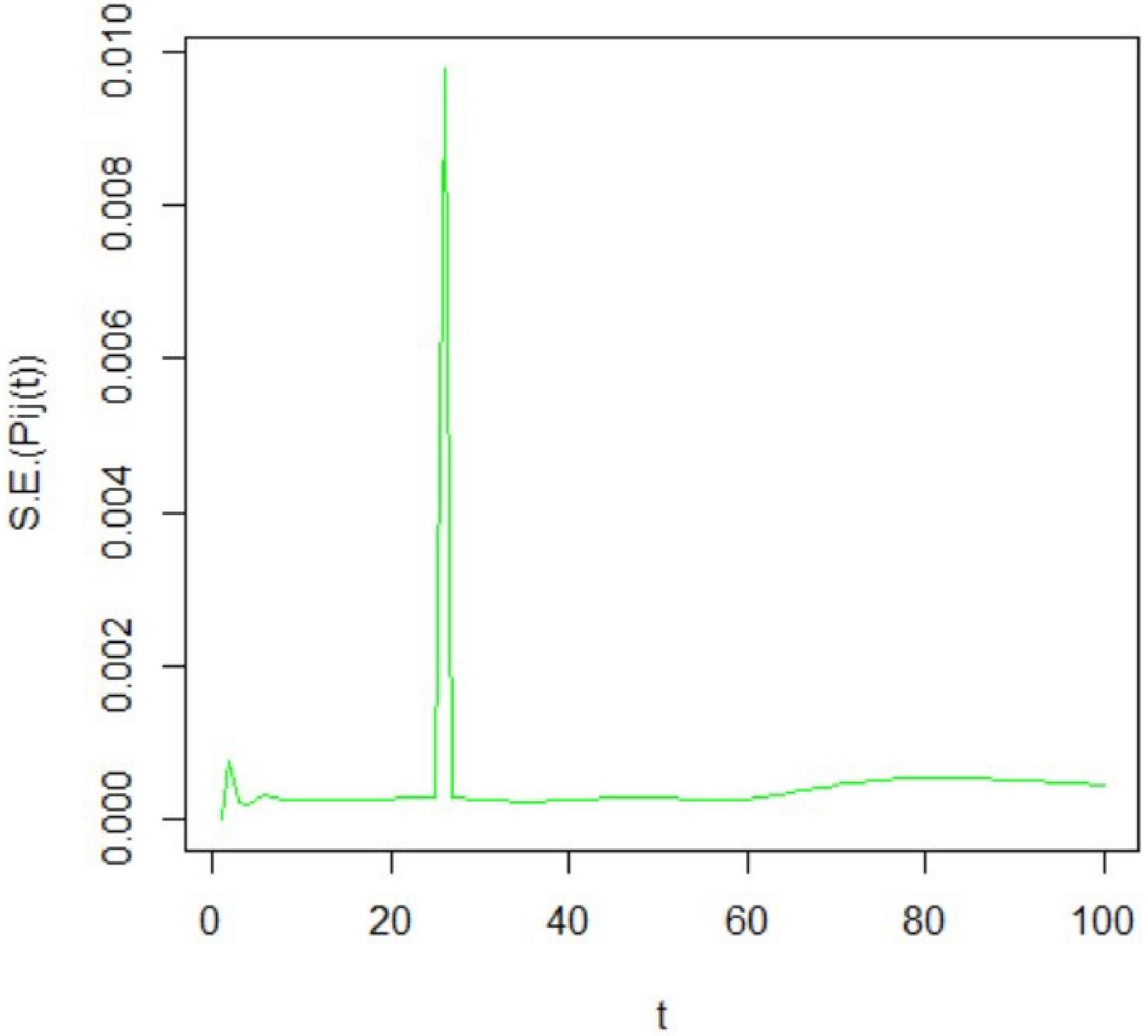
Figure 8 Squared errors of ${\hat{P}}_{i j} (t)$ for uncensored trajectories, for $t \in [1, 2, \dots, 100]$ .

As for the estimator of the initial law (see Figures 3 and 7), in both cases of censoring or not censoring, is close to the vector $(\frac{1}{3}, \frac{1}{3}, \frac{1}{3})$ which is the true value, especially when the number of trajectories is large enough (greater than 30). Figure 8 proves that estimators of the semi-Markov transition probabilities are very accurate with a squared error to be almost zero.

7 Conclusion

A new generalized class of distributions based on the Modified Weibull distribution is proposed in this work where for any specific parent distribution, a new class of distributions is obtained. The aforementioned opens up the way to make inference on a semi-Markov model by allowing a variety of distributions for sojourn times. The main contribution of this work is the fact that using the proposed generalized class we do not limit the problem to a restricted family of distributions. The proposed methodology is examined using simulations providing a comparison between real and estimated parameters with respect to the squared errors. The results are both encouraging and reliable in all cases.

References

[1] Azzalini, A. (1985). A Class of Distributions Which Includes the Normal Ones. Scandinavian Journal of Statistics, 12, 171–178.

[2] Ahuja, J., C. and Nash, Stanley W. (1967). The generalized Gompertz-Verhulst family of distributions. Sankhya, Series A, 29, 141–156.

[3] Balasubramanian, K., Beg, M. I. and Bapat, R. B. (1991). On families of distributions closed under extrema, Sankhya: The Indian Journal of Statistics A, 53, 375–388.

[4] Barbu, V., S., Karagrigoriou, A., Makrides, A. (2017). Semi-Markov Modelling for Multi-State Systems, Meth. & Comput. Appl. Prob., 19, 1011–1028.

[5] Barbu, V., S., Karagrigoriou, A., Makrides, A. (2019). Estimation and reliability for a special type of semi-Markov process, J. Math. Stat., 15(1), 259–272.

[6] Barbu, V., S., Karagrigoriou, A., Makrides, A. (2020). Statistical inference for a general class of distributions with time-varying parameters, J. Appl. Stat., 1–20.

[7] Barbu, V., S., Limnios N. (2004). Discrete time semi-Markov processes for reliability and survival analysis – a nonparametric estimation approach, Parametric and Semiparametric Models with Applications to Reliability, Survival Analysis and Quality of Life, eds. Narayanaswamy Balakrishnan, Mikhail Nikulin, Mounir Mesbah, Nikolaos Limnios, Birkhäuser, Collection Statistics for Industry and Technology, Boston, 487–502.

[8] Delgarm, L. and Zadkarami, M., R. (2015). A new generalization of lifetime distributions, Comput. Stat. 30, 1185–1198.

[9] Eugene N., Lee C., and Famoye F. (2002). Beta-normal distribution and its applications, Commun. Stat. Theory Methods 31, 497–512.

[10] Lai, C., D., Xie, M. and Murthy, D. (2003). A modified Weibull distribution. IEEE Trans. Reliab., 52, 33–37.

[11] Limnios, N. and Oprişan, G. (2001). Semi-Markov Processes and Reliability, Birkhäuser, Boston.

[12] Lisnianski, A., Frenkel, Karagrigoriou A. (2017). Recent advances in multi-state systems reliability: Theory and applications, Springer.

[13] Marshall A., W., Olkin I. (1967). A multivariate exponential distribution. J. Am. Stat. Assoc., 62, 30–44.

[14] Ouhbi, B. and Limnios, N. (1996). Non-parametric estimation for semi-Markov kernels with application to reliability analysis, Appl. Stoch. Models Data Anal., 12, 209–220.

[15] Ristic M., M. and Nadarajah S. (2014). A new lifetime distribution. J. Stat. Comput. Simul. 84, 135–150.

[16] Zografos, K. and Balakrishnan, N. (2009). On families of beta- and generalized gamma-generated distributions and associated inference, Stat. Methodol., 6, 344–362.

Biography

Andreas Makrides is a Post Doc researcher at the Department of Statistics and Actuarial – Financial Mathematics, University of the Aegean, Samos, Greece (advisor: Prof. Alex Karagrigoriou).

His research interests lie among others in Stochastic Modeling, Stochastic Processes, Applied Probability, Mathematical Statistics, Semi-Markov Processes, Reliability Theory, Multi-State Systems, Entropy and Divergence, Goodness of Fit Tests and Control Charts – Statistical Quality Control.

He has worked as a Post Doc researcher (2018–2019) at the Laboratoire de Mathématiques Raphaël Salem, University of Rouen, France.

He received his Ph.D in Statistics (2016) from the Department of Mathematics and Statistics, University of Cyprus, his M.Sc. in Statistics and Modeling (with excellence, 2010) from the Department of Mathematics of Aristotle University of Thessaloniki, Greece and his B.Sc. (Hons, with excellence, 2008) from the Department of Mathematics of Aristotle University of Thessaloniki, Greece.

Andreas has been the representative of both Cyprus and France to the 21st EYSM, July 29–Aug 2, 2019, Belgrade, Serbia (selected by the Regional Committee of the Bernoulli Society). He is the recipient of two excellence awards: (1) IKY (State Scholarships Foundation in Greece) awards, for academic excellence in undergraduate studies during the academic years 2005–2006, 2006–2007, 2007–2008. (2) 1st ranked postgraduate candidate, M.Sc “Statistics and Modeling, Department of Mathematics, Aristotle University of Thessaloniki, Greece, 2008. IKYK (State Scholarships Foundation in Cyprus) Fellowship, for the graduate studies.

He is also a reviewer for several scientific journals.

Furthermore, he has teaching experience since he has been working from 2017 as an Associated Lecturer at the University of Cyprus, the Cyprus University of Technology and the Uclan University, Cyprus on various courses both undergraduate and postgraduate.

Journal of Reliability and Statistical Studies, Vol. 15, Issue 2 (2022), 411–430.
doi: 10.13052/jrss0974-8024.1521
© 2022 River Publishers