A Model for the State of Charge of a Battery Connected to a Wind Power Plant Under a Ramp Rate Limitation Regime

Guglielmo D’Amico¹, Fulvio Gismondi² and Salvatore Vergine^3,*

¹Department of Economics, University G. D’Annunzio, Pescara 65122, Italy
²Department of Economic and Business Science, University G. Marconi, Roma 00193, Italy
³Department of Neurosciences, Imaging and Clinical Sciences, University G. D’Annunzio, Chieti 66100, Italy
E-mail: salvatore.vergine@unich.it
*Corresponding Author

Received 28 December 2021; Accepted 01 May 2022; Publication 22 July 2022

Abstract

In this paper, the expected value of the first hitting time of a threshold of the state of charge of a battery is investigated. The model considers a battery storage system connected to a wind power plant under a ramp rate limitation scheme. The level of charge in the battery is the result of operations that are modelled by a Markov chain model with random rewards. The Markov chain and reward characteristics do depend on the considered ramp rate limitation scheme that the wind power producer has to respect in order to guarantee a quasi-stable output power to the grid. In this paper, we derive a system of integral equations for the hitting time of the state of charge of the battery and the application to real data validates the analytical results.

Keywords: Integral equation, Markov model, battery, wind power.

1 Introduction

One of the main problem of the increasing production of wind power is the injection of electricity into the grid. Sharp variations may induce grid instability. Renewable energy sources are uncontrollable and this fact force the wind farm (WF) to forecast its production. The forecast is always affected by an error and for this motivation the WF needs to find solutions which are generally expensive [1].

One of the possible strategies is to limit the ramp-rate of the wind power [2, 3, 4, 5].

This strategy consists of imposing a limitation to ramp-up and ramp-down events. Precisely, when the wind turbine increases its power production from a time unit to the successive one more than the fixed limitation, the wind power producer (WPP) has to store the excess of production in a storage system or in case of insufficient battery capacity to inject electricity in the grid and suffer a penalty from the controllers of the grid. In the contrary case, when the wind turbine decreases its power more than the limitation, the WPP needs using the battery to supply additional energy to respect the limitation. Also in this case, if the battery does not allow for this operation for insufficient stored energy the WPP will suffer a penalty from the controllers of the grid. The limitation is indicated by a percentage of the maximum ramp rate which can be offered by the wind turbine. Usually, the unit of measure of the ramp rate is MW per minute (MW/min). This method of controlling the wind power output in strongly linked with the necessity to adopt a power storage to produce energy as constant as possible. The main goal is to compensate the variability of the wind power at a reasonable cost, and a lot of control strategies have been studied to find the optimal use of the battery taking into consideration different boundary conditions such as the life of the battery and the state-of-charge (SOC) limits. In particular, it has been shown that the SOC is fundamental not only to immediately respond to energy requests but also because it directly influences the battery functionality [6, 7, 8, 9]. In [10] the authors propose a battery storage scheme composed by two batteries which have the SOC monitored with the aim to obtain the minimum number of the battery switch-overs. In [11] the battery charge is modeled as a fluid into a reservoir where the charge is accumulated or depleted progressively. In [12] a probabilistic approach is used to find the transient solution of the amount of charge into the battery which depends on several input and output processes which in turn depend on the level of charge of the battery.

The Markov reward processes are largely used to study and model the time evolution of a phenomenon [13, 14] and their validity is demonstrated by applying the models to real cases. A general model based on Markov reward chains has been recently proposed by [15]. In that research article the authors were able to compute moments of aggregate discounted penalties over any considered time interval. Based on that recent contribution, here we focus on the expected value of some hitting times of the SOC of the battery. This aspect is crucial in understanding different aspects related to the efficiency of the storage system. Among them we recall the assessment of the battery life and management costs as well as the performance which depends on the level of the SOC of the battery. Moreover, the information provided by our investigation could also be used for the optimal sizing of the storage system, the latter being a relevant recent research subject, see [16]. Our proposal is based on a three state Markov chain model for the battery operations. The states represent the possible operations involving the battery consisting in the charge, discharge of energy or the maintaining of the SOC level. Any operation is represented by a random amount of energy that the battery charge gets accumulated or depleted according to the availability of the battery expressed by the difference between the instantaneous available capacity and the SOC. It should also be remarked that the SOC process is a non-linear function of the random charge/discharge. Our main result is the determination of a system of integral equations expressing the expected value of the hitting time of the fully-charged state and of the empty state of the battery for any initial condition expressed by the battery operation state and the initial value of the SOC process. The solution of the system of integral equations is get numerically by means of a discretization of the SOC process and the approximating linear system of equation is expressed in matrix form. The theoretical results are supported by an empirical investigation on real data. First, we consider 10 years of wind speed data on an hourly base. We implement the model on different scenarios that consider ramp-rate limitations of different percentages ranging from 1% to 5%. We compare the results obtained on real data with those we get from the mathematical model and we conclude that the model can be effectively applied to real cases. The rest of the paper is organized as follows: Section 2 presents the physical problem, the proposed mathematical model and the theoretical and numerical results. Section 3 discusses the real data and the results of the model are compared with the empirical one based on the real data. Section 4 presents some concluding remarks.

2 SOC Modeling

In this section we describe the model on which this study is based on, and subsequently we calculate mathematically the expected value of the fist hitting time of a threshold of the SOC. In the last subsection we show the numerical procedure.

2.1 Probabilistic Model

In this subsection we report the modeling we use to study the phenomenon from the paper [15].

Limiting the ramp rate means making the power produced from a WF more stable and decreasing the variability which intrinsically characterizes it. We indicate with $e(t)$ the power produced from the wind turbine in each time $t$, with $ce(t)$ the power subject to the imposed limitation in each time $t$, and with $lim$ the limitation. $ce(t)$ presents softer fluctuations and less steep slopes compared to $e(t)$. The larger the difference between the two profiles, the stricter is the limitation. To obtain the power $ce(t)$ we use the following formula:

$$ce(t)=\{\begin{array}{cc}\hfill ce(t-1)+lim& \text{if}e(t)>e(t-1)+lim\hfill \\ \hfill ce(t-1)-lim& \text{if}e(t)<e(t-1)-lim\hfill \\ \hfill e(t)& \text{otherwise}\hfill \end{array}$$

(1)

The maximum ramp rate that we can have in this system depends on the considered wind turbines and their rated power. In the applied section it is set to $2$ MW and limiting it means imposing an allowed percentage of $2$ MW/h. The percentage indicates the maximum variation that we can have from an hour to the next one in both cases the power increases and decreases. In particular, the former is called up-ramping limitation and we have a ramp-up event if $e(t)>e(t-1)+lim$, the latter is called down-ramping limitation and we have a ramp-down event if $e(t)<e(t-1)-lim$. By computing the difference between $e(t)$ and $ce(t)$ we know when the battery will charge, discharge and its level of charge will not change (unchanged status), and the corresponding amounts of energy which characterize these situations. At this point we consider the stochastic process ${\{B(t)\}}_{t\in N}$ with values $B(t)\in E=\{+1,0,-1\}$. The quantity $+1$ indicates the situation in which the power is increasing from two consecutive time-steps and the variation is greater that the imposed ramp-rate limitation. This cause a difference between the power profiles $e(t)$ and $ce(t)$ and the excess energy has to be charged into the battery. Vice versa, the quantity $-1$ indicates the situation in which the power is decreasing from two consecutive time-steps and it is not respecting the limitation. In this case the battery has to provide the defect energy to make the system respects the limitation. The quantity $0$ indicates that the variation of the power production is within the allowed range and no operation of charging/discharging the battery is required.

The next step of the model consists of hypothesizing that the vector of states ${\{B(t)\}}_{t\in N}$ is a realization of a discrete time homogeneous Markov chain which has the following transition probability:

	$\mathbb{P}\{B(t+1)=j|B(t)=i_t,B(t-1)=i_{t-1},\mathrm{\dots },B(0)=i_0\}$	(2)
	$=\mathbb{P}\{B(t+1)=j|B(t)=i_t\}=p_{i_t,j}.$

As already described, each value of the process $B(t)$ involves a variation to the battery SOC. We indicate with $R(t)$ the process which describes the theoretical variation of the power into the battery. If $B(t)=+1$, we couple this state with an $R(t)=R_{+1}$ which is a random charge power. Vice versa, if $B(t)=-1$, we couple this state with an $R(t)=R_{-1}$ which is a random discharge power. At this point we hypothesize that the random variable $R(t)$ has a conditional distribution which depends only on the state $B(t)$ in each time step $t\in N$. The following equations indicate this characteristic:

	$F_{+1}(\cdot )=\mathbb{P}(R(t)\le \cdot |B(t)=+1)=\mathbb{P}(R_{+1}\le \cdot ),$	(3)
	$F_{-1}(\cdot )=\mathbb{P}(R(t)\le \cdot |B(t)=-1)=\mathbb{P}(R_{-1}\le \cdot ),$

where $F_{+1}$ and $F_{-1}$ are assumed to be absolutely continuous. For this reason $R_{+1}$ and $R_{-1}$ are random variables having the same cumulative distribution function of $R(t)$ conditional on $B(t)=+1$ and $B(t)=-1$, respectively. We can indicate this in the following way:

	$D(R_{+1}):=D(R(t)|B(t)=+1),$	(4)
	$D(R_{-1}):=D(R(t)|B(t)=-1).$

We get the charge/discharge powers by means of the two distributions $D(R_{+1})$ and $D(R_{-1})$, respectively. These two distributions depend on the state of the underlying Markov chain $B(t)$. They collect possible charge or discharge values depending on the probability distributions of equations (4). We introduce the SOC process $(S(t),t\in N)$ which indicates the level of charge into the battery at each time $t$. Obviously, the SOC of the battery has an upper limit $\overline{c}$ and a lower limit $\underset{¯}{c}$ which are technical constrains. These limits are considered as a percentage of the capacity of the battery.

Considered $S(t-1)=l$ we have the following relation

$$S(t)=\{\begin{array}{cc}\hfill (R_{+1}+l)\wedge \overline{c}\hfill & \text{if}B(t)=+1\hfill \\ \hfill (l-R_{-1})\vee \underset{¯}{c}\hfill & \text{if}B(t)=-1\hfill \\ \hfill l\hfill & \text{if}B(t)=0\text{.}\hfill \end{array}$$

(5)

Thus, when the battery is in the state $+1$, the random power $R_{+1}$ should be stored in the battery. Nevertheless, only the quantity $(R_{+1}+l)\wedge \overline{c}$ can be effectively stored depending on the previous level of the SOC $l$ and on the maximum capacity $\overline{c}$. Contrarily, when the battery is in the state $-1$, the random power $R_{-1}$ should be supplied by the battery. Nevertheless, only the quantity $(l-R_{-1})\vee \underset{¯}{c}$ can be effectively supplied depending on the previous level of the SOC $l$ and on the minimum capacity $\underset{¯}{c}$. Finally, when $B(t)=0$, no charging/discharging operation is required and the SOC remain unchanged to the level $l$.

2.2 The Hitting Times of the SOC of the Battery

In this work we study the expected value of the hitting time of the fully-charged condition and of the empty condition of the battery starting from a given initial SOC.

After defining the state-of-charge process we define the quantity $\tau (\overline{c})$ as follows:

$$\tau (\overline{c})=inf\{t\in \mathbb{N}:S(t)=\overline{c}\},$$

(6)

which is the fist time of the total charge of the battery. Denote by

$$R_{i,l}(\overline{c},m)=\mathbb{P}(\tau (\overline{c})>m\mid B(0)=i,$$
$$S(0)=l)=\mathbb{P}{}_{(i,l)}(\tau (\overline{c})>m),$$	(7)

the corresponding survival function.

We are interested in characterizing the following quantity:

$$a_{i,l}(\overline{c})=𝔼[\tau (\overline{c})\mid B(0)=1,S(0)=l]={𝔼}_{(i,l)}[\tau (\overline{c})].$$

(8)

Being $\tau (\overline{c})$ a discrete random variable, we have that

$$a_{i,l}(\overline{c})={𝔼}_{(i,l)}[\tau (\overline{c})]=\sum _{g\ge 0}{\mathbb{P}}_{(i,l)}[\tau (\overline{c})>g].$$

(9)

It is possible to notice that

${\mathbb{P}}_{(i,l)}(\tau (\overline{c})>m)$	$={\displaystyle \sum _{j\in E}}{\mathbb{P}}_{(i,l)}(\tau (\overline{c})>m,B(1)=j)$	(10)
	$={\displaystyle \sum _{j\in E}}{𝔼}_{(i,l)}[{\mathbb{P}}_{(i,l)}(\tau (\overline{c})>m,$
	$B(1)=j,S(1)<\overline{c}\mid S(1))]$
	$={\displaystyle \sum _{j\in E}}{𝔼}_{(i,l)}[1_{\{S(1)<\overline{c},B(1)=j\}}$
	${\mathbb{P}}_{(j,S(1))}(\tau (\overline{c})>m-1)]$

At this point we use the definition of the SOC in equation (10) and we obtain the following equations:

$\begin{array}{cc}& {𝔼}_{(i,l)}[1_{\{B(1)=1,(R_{+1}+l)\wedge \overline{c}<\overline{c}\}}{\mathbb{P}}_{(+1,R_{+1}+l)\wedge \overline{c})}(\tau (\overline{c})>m-1)]\hfill \\ & +{𝔼}_{(i,l)}[1_{\{B(1)=0,l<\overline{c}\}}{\mathbb{P}}_{(0,l)}(\tau (\overline{c})>m-1)]\hfill \\ & +{𝔼}_{(i,l)}[1_{\{B(1)=-1,(l-R_{-1})\vee \underset{¯}{c}<\overline{c}\}}{\mathbb{P}}_{(-1,l-R_{-1})\vee \underset{¯}{c})}(\tau (\overline{c})>m-1)]\hfill \end{array}$	(11)
$={𝔼}_{(i,l)}[1_{\{B(1)=+1,R_{+1}+l<\overline{c}\}}{\mathbb{P}}_{(+1,R_{+1}+l)}(\tau (\overline{c})>m-1)]$	(12)
$\mathrm{\hspace{1em}\hspace{1em}}+{𝔼}_{(i,l)}[1_{\{B(1)=0,l<\overline{c}\}}{\mathbb{P}}_{(0,l)}(\tau (\overline{c})>m-1)]$	(13)
$\mathrm{\hspace{1em}\hspace{1em}}+{𝔼}_{(i,l)}[1_{\{B(1)=-1,l-R_{-1}<\overline{c}\}}{\mathbb{P}}_{(-1,l-R_{-1})}(\tau (\overline{c})>m-1)].$	(14)

We indicate with $A_{(1)}$, $A_{(2)}$ and $A_{(3)}$ the members (12), (13) and (14), respectively. We find that

$A_{(1)}$	$=p_{i,+1}{\displaystyle {\int }_0^{\overline{c}-l}}\mathit{d}b{f}_{+1}(b)R_{+1,l+b}(\overline{c};m-1),$	(15)
$A_{(2)}$	$=p_{i,0}{R}_{(0,l)}(\overline{c};m-1),$	(16)
$A_{(3)}$	$=p_{i,-1}[{\displaystyle {\int }_0^{l-\underset{¯}{c}}}db{f}_{-1}(b)R_{-1,l-b}(\overline{c};m-1)$
	$\mathrm{\hspace{1em}}+{\overline{F}}_{-1}(l-\underset{¯}{c})R_{-1,\underset{¯}{c}}(\overline{c};m-1)].$	(17)

Since that ${𝔼}_{(i,l)}[\tau (\overline{c})]={\sum }_{m\ge 0}{\mathbb{P}}_{(i,l)}[\tau (\overline{c})>m]$, we can compute the ${\sum }_{m\ge 0}(A_{(1)}+A_{(2)}+A_{(3)})$ and we obtain the following equation:

$\begin{array}{cc}\hfill a_{i,l}(\overline{c})& ={\displaystyle \sum _{m\ge 0}}{p}_{i,+1}{\displaystyle {\int }_0^{\overline{c}-l}}\mathit{d}b{f}_{+1}(b)R_{+1,l+b}(\overline{c};m-1)\hfill \\ & +{\displaystyle \sum _{m\ge 0}}{p}_{i,0}{R}_{(0,l)}(\overline{c};m-1)\hfill \\ & +{\displaystyle \sum _{m\ge 0}}{p}_{i,-1}[{\displaystyle {\int }_0^{l-\underset{¯}{c}}}db{f}_{-1}(b)R_{-1,l-b}(\overline{c};m-1)+{\overline{F}}_{-1}(l-\underset{¯}{c})\hfill \\ & R_{-1,\underset{¯}{c}}(\overline{c};m-1)].\hfill \end{array}$

(18)

We set $h=m-1$ and we observe that

${\displaystyle \sum _{m\ge 0}}{R}_{\cdot ,\cdot }(\overline{c};m-1)$	$={\displaystyle \sum _{h+1\ge 0}}{R}_{\cdot ,\cdot }(\overline{c};h)$	(19)
	$={\displaystyle \sum _{h\ge -1}}{R}_{\cdot ,\cdot }(\overline{c};h)=1+{\displaystyle \sum _{h\ge 0}}{R}_{\cdot ,\cdot }(\overline{c};h)=1+a_{\cdot ,\cdot }(\overline{c}).$

Therefore, we obtain that

$a_{i,l}(\overline{c})$	$=p_{i,+1}{\displaystyle {\int }_0^{\overline{c}-l}}db{f}_{+1}(b)(1+a_{+1,l+b}(\overline{c})+p_{i,0}[1+a_{0,l}(\overline{c})]$
	$\mathrm{\hspace{1em}}+p_{i,-1}[{\displaystyle {\int }_0^{l-\underset{¯}{c}}}db{f}_{-1}(b)[1+a_{-1,l-b}(\overline{c})]$
	$\mathrm{\hspace{1em}}+{\overline{F}}_{-1}(l-\underset{¯}{c})[1+a_{-1,\underset{¯}{c}}(\overline{c})]].$	(20)

From the equation (2.2) we have the following equation

$a_{i,l}(\overline{c})$	$=p_{i,+1}{F}_{+1}(\overline{c}-l)$
	$\mathrm{\hspace{1em}}+p_{i,+1}{\displaystyle {\int }_0^{\overline{c}-l}}\mathit{d}b{f}_{+1}(b)\cdot a_{+1,l+b}(\overline{c})+p_{i,0}(1+a_{0,l}(\overline{c}))$
	$\mathrm{\hspace{1em}}+p_{i,-1}(F_{-1}(l-\underset{¯}{c})$
	$\mathrm{\hspace{1em}}+{\displaystyle {\int }_0^{l-\underset{¯}{c}}}\mathit{d}b{f}_{-1}(b)\cdot a_{-1,l-b}(\overline{c})+{\overline{F}}_{-1}(l-\underset{¯}{c})$
	$\mathrm{\hspace{1em}}+{\overline{F}}_{-1}(l-\underset{¯}{c})\cdot a_{-1,\underset{¯}{c}}(\overline{c})).$	(21)

By observing that $F_{-1}(l-\underset{¯}{c})+{\overline{F}}_{-1}(l-\underset{¯}{c})=1$ we get the equation (22)

$a_{i,l}(\overline{c})$	$=p_{i,+1}\cdot F_{+1}(\overline{c}-l)$	(22)
	$+p_{i,+1}\cdot {\displaystyle {\int }_0^{\overline{c}-l}}\mathit{d}b{f}_{+1}(b)\cdot a_{+1,l+b}(\overline{c})+p_{i,0}+p_{i,0}\cdot a_{0,l}(\overline{c})$
	$+p_{i,-1}\left(1+{\displaystyle {\int }_0^{l-\underset{¯}{c}}}\mathit{d}b{f}_{-1}(b)\cdot a_{-1,l-b}(\overline{c})+{\overline{F}}_{-1}(l-\underset{¯}{c})\cdot a_{-1,\underset{¯}{c}}(\overline{c})\right).$

As the value of $i\in \{+1,0,-1\}$, we obtain a system of three integral equations with unknown functions $a_{1,\cdot }(\overline{c})$, $a_{0,\cdot }(\overline{c})$, $a_{-1,\cdot }(\overline{c})$.

At this point we provide an explicit representation of the system of equations.

$a_{1,l}(\overline{c})$	$=p_{1,1}\cdot F_1(\overline{c}-l)+p_{1,1}{\displaystyle {\int }_0^{\overline{c}-l}}\mathit{d}b{f}_{+1}(b)a_{+1,l+b}(\overline{c})$
	$\mathrm{\hspace{1em}}+p_{1,0}+p_{1,0}\cdot a_{0,l}(\overline{c})$
	$\mathrm{\hspace{1em}}+p_{1,-1}(1+{\displaystyle {\int }_0^{l-\underset{¯}{c}}}db{f}_{-1}(b)\cdot a_{-1,l-b}(\overline{c})$
	$\mathrm{\hspace{1em}}+{\overline{F}}_{-1}(l-\underset{¯}{c})a_{-1,\underset{¯}{c}}(\overline{c})),$
$a_{0,l}(\overline{c})$	$=p_{0,1}\cdot F_1(\overline{c}-l)+p_{0,1}{\displaystyle {\int }_0^{\overline{c}-l}}\mathit{d}b{f}_{+1}(b)\cdot a_{+1,l+b}(\overline{c})$
	$\mathrm{\hspace{1em}}+p_{0,0}+p_{0,0}\cdot a_{0,l}(\overline{c})$
	$\mathrm{\hspace{1em}}+p_{0,-1}(1+{\displaystyle {\int }_0^{l-\underset{¯}{c}}}db{f}_{-1}(b)\cdot a_{-1,l-b}(\overline{c})$
	$\mathrm{\hspace{1em}}+{\overline{F}}_{-1}(l-\underset{¯}{c})a_{-1,\underset{¯}{c}}(\overline{c})),$
$a_{-1,l}(\overline{c})$	$=p_{-1,1}\cdot F_1(\overline{c}-l)+p_{-1,1}{\displaystyle {\int }_0^{\overline{c}-l}}\mathit{d}b{f}_{+1}(b)\cdot a_{+1,l+b}(\overline{c})$
	$\mathrm{\hspace{1em}}+p_{-1,0}+p_{-1,0}\cdot a_{0,l}(\overline{c})$
	$\mathrm{\hspace{1em}}+p_{-1,-1}(1+{\displaystyle {\int }_0^{l-\underset{¯}{c}}}db{f}_{-1}(b)\cdot a_{-1,l-b}(\overline{c})$
	$\mathrm{\hspace{1em}}+{\overline{F}}_{-1}(l-\underset{¯}{c})a_{-1,\underset{¯}{c}}(\overline{c})).$	(23)

Before finding the system solutions, we note that the term $a_{0,l}(\overline{c})$ appears in all the equations. Indeed, from the first equation we have

$a_{0,l}(\overline{c})$	$={\displaystyle \frac{1}{p_{1,0}}}\{a_{1,l}(\overline{c})-p_{1,1}\cdot F_1(\overline{c}-l)$	(24)
	$-p_{1,1}{\displaystyle {\int }_0^{\overline{c}-l}}\mathit{d}b{f}_{+1}(b)\cdot a_{+1,l+b}(\overline{c})-p_{1,0}$
	$-p_{1,-1}(1+{\displaystyle {\int }_0^{l-\underset{¯}{c}}}db{f}_{-1}(b)\cdot a_{-1,l-b}(\overline{c})$
	$+{\overline{F}}_{-1}(l-\underset{¯}{c})\cdot a_{-1,\underset{¯}{c}}(\overline{c}))\}.$

The second equation gives

$a_{0,l}(\overline{c})$	$={\displaystyle \frac{1}{1-p_{0,0}}}$	(25)
	$\times \{p_{0,1}{F}_1(\overline{c}-l)+p_{0,1}{\displaystyle {\int }_0^{\overline{c}-l}}db{f}_{+1}(b)\cdot a_{+1,l+b}(\overline{c})$
	$+p_{0,0}+p_{0,-1}$
	$\times (1+{\displaystyle {\int }_0^{l-\underset{¯}{c}}}db{f}_{-1}(b)\cdot a_{-1,l-b}(\overline{c})+{\overline{F}}_{-1}(l-\underset{¯}{c})\cdot a_{-1,\underset{¯}{c}}(\overline{c}))\}.$

The third equation gives

$a_{0,l}(\overline{c})$	$={\displaystyle \frac{1}{p_{-1,0}}}\{a_{-1,l}(\overline{c})-p_{-1,1}{F}_1(\overline{c}-l)$	(26)
	$-p_{-1,1}{\displaystyle {\int }_0^{\overline{c}-l}}\mathit{d}b{f}_{+1}(b)\cdot a_{+1,l+b}(\overline{c})-p_{-1,0}$
	$-p_{-1,-1}(1+{\displaystyle {\int }_0^{l-\underset{¯}{c}}}db{f}_{-1}(b)a_{-1,l-b}(\overline{c})$
	$+{\overline{F}}_{-1}(l-\underset{¯}{c})a_{-1,\underset{¯}{c}}(\overline{c}))\}.$

If we equate the equation (24) with the equation (25) we obtain that

	$a_{1,l}(\overline{c})-p_{1,1}\cdot F_1(\overline{c}-l)-p_{1,1}{\displaystyle {\int }_0^{\overline{c}-l}}\mathit{d}b{f}_{+1}(b)\cdot a_{+1,l+b}(\overline{c})-p_{1,0}$	(27)
	$-p_{1,-1}\left(1+{\displaystyle {\int }_0^{l-\underset{¯}{c}}}\mathit{d}b{f}_{-1}(b)\cdot a_{-1,l-b}(\overline{c})+{\overline{F}}_{-1}(l-\underset{¯}{c})\cdot a_{-1,\underset{¯}{c}}(\overline{c})\right)$
	$-{\displaystyle \frac{p_{1,0}\cdot p_{0,1}}{1-p_{0,0}}}{F}_1(\overline{c}-l)-{\displaystyle \frac{p_{0,1}\cdot p_{1,0}}{1-p_{0,0}}}{\displaystyle {\int }_0^{\overline{c}-l}}\mathit{d}b{f}_{+1}(b)\cdot a_{+1,l+b}(\overline{c})$
	$-{\displaystyle \frac{p_{1,0}\cdot p_{0,0}}{1-p_{0,0}}}-{\displaystyle \frac{p_{1,0}\cdot p_{0,-1}}{1-p_{0,0}}}(1+{\displaystyle {\int }_0^{l-\underset{¯}{c}}}db{f}_{-1}(b)a_{-1,l-b}(\overline{c})$
	$+{\overline{F}}_{-1}(l-\underset{¯}{c})a_{-1,\underset{¯}{c}}(\overline{c}))=0,$

that is

	$a_{1,l}(\overline{c})-\left[p_{1,1}+{\displaystyle \frac{p_{1,0}\cdot p_{0,1}}{1-p_{0,0}}}\right]F_1(\overline{c}-l)$	(28)
	$-\left[p_{1,1}+{\displaystyle \frac{p_{1,0}\cdot p_{0,1}}{1-p_{0,0}}}\right]{\displaystyle {\int }_0^{\overline{c}-l}}\mathit{d}b{f}_{+1}(b)a_{+1,l+b}(\overline{c})$
	$-\left[p_{1,0}+{\displaystyle \frac{p_{1,0}\cdot p_{0,0}}{1-p_{0,0}}}\right]-[p_{1,-1}+{\displaystyle \frac{p_{1,0}\cdot p_{0,-1}}{1-p_{0,0}}}]$
	$\cdot (1+{\displaystyle {\int }_0^{l-\underset{¯}{c}}}db{f}_{-1}(b)a_{-1,l-b}(\overline{c})+{\overline{F}}_{-1}(l-\underset{¯}{c})a_{-1,\underset{¯}{c}}(\overline{c}))=0.$

In this way we obtain the following equation:

$a_{1,l}(\overline{c})$	$=\left[p_{1,1}+{\displaystyle \frac{p_{1,0}\cdot p_{0,1}}{1-p_{0,0}}}\right](F_1(\overline{c}-l)+{\displaystyle {\int }_0^{\overline{c}-l}}\mathit{d}b{f}_{+1}(b)\cdot a_{+1,l+b}(\overline{c}))$	(29)
	$+\left[p_{1,0}+{\displaystyle \frac{p_{1,0}\cdot p_{0,0}}{1-p_{0,0}}}\right]+\left[p_{1,-1}+{\displaystyle \frac{p_{1,0}\cdot p_{0,-1}}{1-p_{0,0}}}\right]$
	$\cdot \left(1+{\displaystyle {\int }_0^{l-\underset{¯}{c}}}\mathit{d}b{f}_{-1}(b)\cdot a_{-1,l-b}(\overline{c})+{\overline{F}}_{-1}(l-\underset{¯}{c})\cdot a_{-1,\underset{¯}{c}}(\overline{c})\right).$

By equaling the Equation (25) with the Equation (26) we obtain the following equation:

	$a_{-1,l}(\overline{c})-p_{-1,1}\left(F_1(\overline{c}-l)+{\displaystyle {\int }_0^{\overline{c}-l}}\mathit{d}b{f}_{+1}(b)\cdot a_{+1,l+b}(\overline{c})\right)-p_{-1,0}$	(30)
	$-p_{-1,1}\left(1+{\displaystyle {\int }_0^{l-\underset{¯}{c}}}\mathit{d}b{f}_{-1}(b)\cdot a_{-1,l-b}(\overline{c})+{\overline{F}}_{-1}(l-\underset{¯}{c})a_{-1,\underset{¯}{c}}(\overline{c})\right)$
	$={\displaystyle \frac{p_{-1,0}}{1-p_{0,0}}}\{p_{0,1}\cdot [F_1(\overline{c}-l)+{\displaystyle {\int }_0^{\overline{c}-l}}db{f}_{+1}(b)a_{+1,l+b}(\overline{c})]+p_{0,0}$
	$+p_{0,-1}(1+{\displaystyle {\int }_0^{l-\underset{¯}{c}}}db{f}_{-1}(b)\cdot a_{-1,l-b}(\overline{c})+{\overline{F}}_{-1}(l-\underset{¯}{c})a_{-1,\underset{¯}{c}}(\overline{c}))\}.$

At this point we get $a_{-1,l}(\overline{c})$:

$a_{-1,l}(\overline{c})$	$=\left[p_{-1,1}+{\displaystyle \frac{p_{-1,0}\cdot p_{0,1}}{1-p_{0,0}}}\right]$	(31)
	$\cdot \left(F_1(\overline{c}-l)+{\displaystyle {\int }_0^{\overline{c}-l}}\mathit{d}b{f}_{+1}(b)\cdot a_{+1,l+b}(\overline{c})\right)$
	$+\left[p_{-1,0}+{\displaystyle \frac{p_{-1,0}\cdot p_{0,0}}{1-p_{0,0}}}\right]$
	$+\left[p_{-1,-1}+{\displaystyle \frac{p_{-1,0}\cdot p_{0,-1}}{1-p_{0,0}}}\right]$
	$\cdot \left(1+{\displaystyle {\int }_0^{l-\underset{¯}{c}}}\mathit{d}b{f}_{-1}(b)a_{-1,l-b}(\overline{c})+{\overline{F}}_{-1}(l-\underset{¯}{c})a_{-1,\underset{¯}{c}}(\overline{c})\right).$

The term $a_{0,\cdot }(\overline{c})$ does not appear in the equations (29) and (31), hence we have obtained a system composed by two equations with two unknown variables, $a_{-1,\cdot }(\overline{c})$ and $a_{1,\cdot }(\overline{c})$. In this way we can calculate $a_{0,\cdot }(\overline{c})$ from the equations (2.2). We may simplify the writing by considering $t_{i,j}:=p_{i,j}+\frac{p_{i,0}\cdot p_{0,j}}{1-p_{0,0}}$ $\forall i,j\in E$ and we obtain the following system of two integral equations which can be claimed as follows

Proposition 1 The expected value of the first hitting time of the total charge of the battery satisfies the next system of integral equations

$$\{\begin{array}{cc}\hfill a_{1,l}(\overline{c})& =[t_{1,1}\cdot F_1(\overline{c}-l)+t_{1,0}+t_{1,-1}]\hfill \\ & +t_{1,1}\cdot {\int }_0^{\overline{c}-l}\mathit{d}b{f}_{+1}(b)\cdot a_{+1,l+b}(\overline{c})\hfill \\ & +t_{1,-1}{\int }_0^{l-\underset{¯}{c}}\mathit{d}b{f}_{-1}(b)\cdot a_{-1,l-b}(\overline{c})\hfill \\ & +t_{1,-1}{\overline{F}}_{-1}(l-\underset{¯}{c})a_{-1,\underset{¯}{c}}(\overline{c})\hfill \\ & \\ \hfill a_{-1,l}(\overline{c})& =[t_{-1,1}\cdot F_1(\overline{c}-l)+t_{-1,0}+t_{-1,-1}]\hfill \\ & +t_{-1,1}\cdot {\int }_0^{\overline{c}-l}\mathit{d}b{f}_{+1}(b)\cdot a_{+1,l+b}(\overline{c})\hfill \\ & +t_{-1,-1}{\int }_0^{l-\underset{¯}{c}}\mathit{d}b{f}_{-1}(b)\cdot a_{-1,l-b}(\overline{c})\hfill \\ & +t_{-1,-1}{\overline{F}}_{-1}(l-\underset{¯}{c})a_{-1,\underset{¯}{c}}(\overline{c})\hfill \end{array}$$

(32)

while $a_{\mathrm{0}\mathrm{,}l}\mathit{}\mathrm{(}\overline{c}\mathrm{)}$ can be recovered from relation (24) once the system (32) has been solved.

In the same way we can define $\tau (\underset{¯}{c})=inf\{t\in \mathbb{N}:S(t)=\underset{¯}{c}\}$ the first time of total discharging of the battery. With

$$R_{i,l}(\underset{¯}{c};m)=\mathbb{P}(\tau (\underset{¯}{c})>m|B(0)=i,S(0)=l)={\mathbb{P}}_{(i,l)}(\tau (\underset{¯}{c})>m),$$

we denote its conditional survival function. Let

$$a_{i,l}(\underset{¯}{c})=𝔼[\tau (\underset{¯}{c})|B(0)=i,S(0)=l]={𝔼}_{(i,l)}[\tau (\underset{¯}{c})]$$

(33)

in a similar way we obtain

$$a_{i,l}(\underset{¯}{c})=\sum _{g\ge 0}{\mathbb{P}}_{(i,l)}[\tau (\underset{¯}{c})>g]$$

(34)

$$\begin{array}{cc}\hfill {\mathbb{P}}_{i,l}[\tau (\underset{¯}{c})>g]& =\sum _{j\in E}{\mathbb{P}}_{(i,l)}(\tau (\underset{¯}{c})>m,B(1)=j)\hfill \\ & =\sum _{j\in E}{𝔼}_{(i,l)}[{\mathbb{P}}_{(i,l)}(\tau (\underset{¯}{c})>m,B(1)=j,S(1)>\underset{¯}{c}|S(1))]\hfill \\ & =\sum _{j\in E}{𝔼}_{(i,l)}[1_{\{S(1)>\underset{¯}{c},B(1)=j\}}{\mathbb{P}}_{(j,S(1))}(\tau (\underset{¯}{c})>m-1)].\hfill \end{array}$$

(35)

We can use the definition of the SOC process to have the following result:

$$\begin{array}{cc}& {\mathbb{P}}_{(i,l)}[\tau (\underset{¯}{c})>g]\hfill \\ & ={𝔼}_{(i,l)}[1_{\{B(1)=1,(R_{+1}+l)\wedge \overline{c}>\underset{¯}{c}\}}{\mathbb{P}}_{(+1,(R_{+1}+l)\wedge \overline{c})}(\tau (\underset{¯}{c})>m-1)]\hfill \\ & +{𝔼}_{(i,l)}[1_{\{B(1)=0,l>\underset{¯}{c}\}}{\mathbb{P}}_{(0,l)}(\tau (\underset{¯}{c})>m-1)]\hfill \\ & +{𝔼}_{(i,l)}[1_{\{B(1)=-1,(l-R_{-1})\vee \underset{¯}{c}>\underset{¯}{c}\}}{\mathbb{P}}_{(-1,(l-R_{-1})\vee \underset{¯}{c})}(\tau (\underset{¯}{c})>m-1)]\hfill \end{array}$$	(36)
$$={𝔼}_{(i,l)}[1_{\{B(1)=1,(R_{+1}+l)>\underset{¯}{c}\}}{\mathbb{P}}_{(+1,(R_{+1}+l)}(\tau (\underset{¯}{c})>m-1)]$$	(37)
$$+{𝔼}_{(i,l)}[1_{\{B(1)=0,l>\underset{¯}{c}\}}{\mathbb{P}}_{(0,l)}(\tau (\underset{¯}{c})>m-1)]$$	(38)
$$+{𝔼}_{(i,l)}[1_{\{B(1)=-1,l-R_{-1}>\underset{¯}{c}\}}{\mathbb{P}}_{(-1,l-R_{-1})}(\tau (\underset{¯}{c})>m-1)]$$	(39)

We name the equations (37), (38) and (39), $B_1$, $B_2$, and $B_3$, respectively.

We can write the following equation:

$$B_1=p_{i,+1}\cdot {\int }_0^{\mathrm{\infty }}\mathit{d}b{f}_{+1}(b)\cdot R_{+1,b+l}(\underset{¯}{c};m-1).$$

(40)

We observe that $R_{+1,l}(\underset{¯}{c};m)$ is defined only into the interval $l\in [\underset{¯}{c},\overline{c}]$. Therefore, we obtain:

$B_1$	$=p_{i,+1}\cdot ({\displaystyle {\int }_0^{\overline{c}-l}}db{f}_{+1}(b)\cdot R_{+1,b+l}(\underset{¯}{c};m-1)$	(41)
	$+{\displaystyle {\int }_{\overline{c}-l}^{\mathrm{\infty }}}db{f}_{+1}(b)\cdot R_{+1,b+l}(\underset{¯}{c};m-1))$
	$=p_{i,+1}\cdot ({\displaystyle {\int }_0^{\overline{c}-l}}db{f}_{+1}(b)\cdot R_{+1,b+l}(\underset{¯}{c};m-1)$
	$+{\overline{F}}_{+1}(\overline{c}-l)\cdot R_{+1,\overline{c}}(\underset{¯}{c};m-1)).$

We can also obtain the quantities $B_2$ and $B_3$.

$$B_2=p_{i,0}\cdot R_{0,l}(\underset{¯}{c};m-1)).$$	(42)
$$B_3=p_{i,-1}\cdot {\int }_0^{l-\underset{¯}{c}}\mathit{d}b{f}_{-1}\cdot R_{-1,l-b}(\underset{¯}{c};m-1).$$	(43)

At this point apply with ${\sum }_{m\ge 0}(B_1+B_2+B_3)$ to get

$a_{i,l}(\underset{¯}{c})$	$={\displaystyle \sum _{m\ge 0}}\{p_{i,+1}\cdot ({\displaystyle {\int }_0^{\overline{c}-l}}db{f}_{+1}(b)\cdot R_{+1,l+b}(\underset{¯}{c};m-1)$	(44)
	$+{\overline{F}}_{+1}(\overline{c}-l)\cdot R_{+1,\overline{c}}(\underset{¯}{c};m-1))+p{}_{i,0}\cdot R{}_{0,l}(\underset{¯}{c};m-1)$
	$+p_{i,-1}{\displaystyle {\int }_0^{l-\underset{¯}{c}}}db{f}_{-1}(b)\cdot R_{-1,l-b}(\underset{¯}{c};m-1)\}.$

We put $h=m-1$ and we observe that

	${\displaystyle \sum _{m\ge 0}}{R}_{\cdot ,\cdot }(\underset{¯}{c};m-1)={\displaystyle \sum _{h+1\ge 0}}{R}_{\cdot ,\cdot }(\underset{¯}{c};h)$	(45)
	$={\displaystyle \sum _{h\ge -1}}{R}_{\cdot ,\cdot }(\underset{¯}{c};h)=1+{\displaystyle \sum _{h\ge 0}}{R}_{\cdot ,\cdot }(\underset{¯}{c};h)=1+a_{\cdot ,\cdot }(\underset{¯}{c}).$

Therefore, we obtain the following equation:

$a_{i,l}(\underset{¯}{c})$	$=p_{i,+1}\cdot ({\displaystyle {\int }_0^{\overline{c}-l}}db{f}_{+1}(b)\cdot (1+a_{1,l+b}(\underset{¯}{c}))$	(46)
	$+{\overline{F}}_{+1}(\overline{c}-l)\cdot (1+a_{+1,\overline{c}}(\underset{¯}{c})))$
	$+p_{i,0}\cdot (1+a_{0,l}(\underset{¯}{c}))+p_{i,-1}\cdot {\displaystyle {\int }_0^{l-\underset{¯}{c}}}\mathit{d}b{f}_{-1}(b)\cdot (1+a_{-1,l-b}(\underset{¯}{c}))$
	$=p_{i,+1}\cdot ({\displaystyle {\int }_0^{\overline{c}-l}}db{f}_{+1}(b)\cdot a_{1,l+b}(\underset{¯}{c})$
	$+F_{+1}(\overline{c}-l)+{\overline{F}}_{+1}(\overline{c}-l)+{\overline{F}}_{+1}(\overline{c}-l)\cdot a_{+1,\overline{c}}(\underset{¯}{c}))$
	$+p_{i,0}+p_{i,0}\cdot a_{0,l}(\underset{¯}{c})+p_{i,-1}{F}_{-1}(l-\underset{¯}{c})$
	$+p_{i,-1}{\displaystyle {\int }_0^{l-\underset{¯}{c}}}\mathit{d}b{f}_{-1}(b)a_{-1,l-b}(\underset{¯}{c}).$

The previous equation is equivalent to the following:

$a_{i,l}(\underset{¯}{c})$	$=p_{i,+1}\cdot {\displaystyle {\int }_0^{\overline{c}-l}}\mathit{d}b{f}_{+1}(b)\cdot a_{1,l+b}(\underset{¯}{c})+p_{i,+1}$	(47)
	$+p_{i,+1}\cdot {\overline{F}}_{+1}(\overline{c}-l)\cdot a_{+1,\overline{c}}(\underset{¯}{c})+p_{i,0}+p_{i,0}\cdot (a_{0,l}(\underset{¯}{c}))$
	$+p_{i,-1}\cdot F_{-1}(l-\underset{¯}{c})+p_{i,-1}\cdot {\displaystyle {\int }_0^{l-\underset{¯}{c}}}\mathit{d}b{f}_{-1}(b)\cdot a_{-1,l-b}(\underset{¯}{c}).$

As we vary $i\in \{+1,0,-1\}$ we obtain the system composed by the following three equations:

$a_{1,l}(\underset{¯}{c})$	$=p_{1,1}\cdot \left(1+{\displaystyle {\int }_0^{\overline{c}-l}}\mathit{d}b{f}_{+1}(b)\cdot a_{1,l+b}(\underset{¯}{c})+{\overline{F}}_{+1}(\overline{c}-l)\cdot a_{+1,\overline{c}}(\underset{¯}{c})\right)$	(48)
	$+p_{1,0}+p_{1,0}\cdot a_{0,l}(\underset{¯}{c})+p_{1,-1}\cdot F_{-1}(l-\underset{¯}{c})$
	$+p_{1,-1}\cdot {\displaystyle {\int }_0^{l-\underset{¯}{c}}}\mathit{d}b{f}_{-1}(b)\cdot a_{-1,l-b}(\underset{¯}{c})$

$a_{0,l}(\underset{¯}{c})$	$=p_{0,1}\cdot \left(1+{\displaystyle {\int }_0^{\overline{c}-l}}\mathit{d}b{f}_{+1}(b)\cdot a_{1,l+b}(\underset{¯}{c})+{\overline{F}}_{+1}(\overline{c}-l)\cdot a_{+1,\overline{c}}(\underset{¯}{c})\right)$	(49)
	$+p_{0,0}+p_{0,0}\cdot a_{0,l}(\underset{¯}{c})+p_{0,-1}\cdot F_{-1}(l-\underset{¯}{c})$
	$+p_{0,-1}\cdot {\displaystyle {\int }_0^{l-\underset{¯}{c}}}\mathit{d}b{f}_{-1}(b)\cdot a_{-1,l-b}(\underset{¯}{c})$

$a_{-1,l}(\underset{¯}{c})$	$=p_{-1,1}\cdot {\displaystyle {\int }_0^{\overline{c}-l}}\mathit{d}b{f}_{+1}(b)\cdot a_{1,l+b}(\underset{¯}{c})+p_{-1,1}$	(50)
	$+p_{-1,1}\cdot {\overline{F}}_{+1}(\overline{c}-l)\cdot a_{+1,\overline{c}}(\underset{¯}{c})+p_{-1,0}+p_{-1,0}\cdot a_{0,l}(\underset{¯}{c})$
	$+p_{-1,-1}\cdot F_{-1}(l-\underset{¯}{c})+p_{-1,-1}\cdot {\displaystyle {\int }_0^{l-\underset{¯}{c}}}\mathit{d}b{f}_{-1}(b)\cdot a_{-1,l-b}(\underset{¯}{c})$

Similar calculations as we did before for the system of expected values of the first hitting time of complete charge of the battery, can reduce the system to only two equations with unknown functions $a_{+1,\cdot }(\underset{¯}{c})$, $a_{-1,\cdot }(\underset{¯}{c})$ and a formula expressing $a_{0,\cdot }(\underset{¯}{c})$ depending on the two previous unknowns.

Remark 1 It is worth noting that the problem can be extended to build more complex models with more than $\mathrm{3}$ states. An example is represented when the hybrid plant has several batteries and each of them has a specific charge/discharge policy. This more complex framework can be managed with the introduction of more states but the mathematical apparatus remains almost unchanged.

2.3 Numerical Solution Method

To solve the system (32) we proceed numerically by means of a discretization. We consider the interval $[0,\overline{c}]$ which indicated the possible values of energy to be charged or discharged into the battery and we discretize it by introducing a grid of $n$ intervals of amplitude $\delta =\frac{\overline{c}}{n}$.

Let ${\{s_i\}}_{i=0}^n$ be the $n+1$ points of the partition. We observe that $s_0=0$, $s_i=s_{i-1}+\delta$ $\forall i=1,..,n$, and $s_n=\overline{c}$.

In general, let $\varphi :[0,\overline{c}]$ $\to ℝ$ be any real valued function and let consider its approximation over the grid ${\{s_i\}}_{i=0}^n$ as follows:

$$\varphi (l)=\{\begin{array}{cc}\hfill \varphi (\overline{c})\hfill & \text{if}l=\overline{c}=s_n\hfill \\ \hfill \varphi (s_{h-1})\hfill & \text{if}{s}_{h-1}\le l<s_h\forall i=1,..,n\text{.}\hfill \end{array}$$

(51)

Consequentially, we can approximate the functions of the system as follows:

	${\displaystyle {\int }_0^{\overline{c}-l}}\mathit{d}b{f}_{+1}(b)\cdot a_{+1,l+b}(\overline{c})$	(52)
	$\approx {\displaystyle \sum _{k=1}^{n-[l]}}{\displaystyle \frac{F_1(s_k)-F_1(s_{k-1})}{\delta }}{a}_{+1,s_{[l]}+k\delta }(\overline{c})$
	$\text{where}[l]=\max \{i:s_i\le l\}.$

	${\displaystyle {\int }_0^{l-\underset{¯}{c}}}\mathit{d}b{f}_{-1}(b)\cdot a_{-1,l-b}(\overline{c})\approx {\displaystyle \sum _{k=1}^{[l]-[\underset{¯}{c}]}}{\displaystyle \frac{F_{-1}(s_k)-F_{-1}(s_{k-1})}{\delta }}{a}_{-1,s_{[l]}-k\delta }(\overline{c})$	(53)
	where $[\underset{¯}{c}]=\max \{i:s_i\le \underset{¯}{c}\}$

$${\overline{F}}_{-1}(l-\underset{¯}{c})a_{-1,\underset{¯}{c}}(\overline{c})\approx F_{-1}(s_{[l]}-s_{[\underset{¯}{c}]})a_{-1,s_{[\underset{¯}{c}]}}(\overline{c}).$$

(54)

By putting $[l]=s_{[\underset{¯}{c}]},s_{[\underset{¯}{c}]+1},..,s_{n-1}$, we obtain a system with $2\cdot (n-[\underset{¯}{c}])$ equations in $2\cdot (n-[\underset{¯}{c}])$ unknown variables $a_{i,s_j}(\overline{c})$ with $i\in \{+1,-1\}$ and $j\in \{[\underset{¯}{c}],[\underset{¯}{c}]+1,..,n-1\}$.

For completeness, we write again the the discrete system:

$a_{1,s_{[\underset{¯}{c}]}}(\overline{c})$	$=[t_{1,1}{F}_1(s_n-s_{[\underset{¯}{c}]})+t_{1,0}+t_{1,-1}]$
	$\mathrm{\hspace{1em}}+t_{1,1}{\displaystyle \sum _{k=1}^{n-[\underset{¯}{c}]}}{\displaystyle \frac{F_1(s_k)-F_1(s_{k-1})}{\delta }}{a}_{+1,s_{[\underset{¯}{c}]}+k\delta }(\overline{c})$
	$\mathrm{\hspace{1em}}+0+t_{1,-1}\cdot 1\cdot a_{-1,s_{[\underset{¯}{c}]}}(\overline{c})$	(55)

$a_{1,s_{[\underset{¯}{c}]}+1}(\overline{c})$	$=[t_{1,1}{F}_1(s_n-s_{[\underset{¯}{c}]+1})+t_{1,0}+t_{1,-1}]$	(56)
	$+t_{1,1}{\displaystyle \sum _{k=1}^{n-([\underset{¯}{c}]+1)}}{\displaystyle \frac{F_1(s_k)-F_1(s_{k-1})}{\delta }}{a}_{+1,s_{[\underset{¯}{c}]+1}+k\delta }(\overline{c})$
	$+t_{1,-1}\cdot {\displaystyle \sum _{k=1}^{[\underset{¯}{c}]+1-[\underset{¯}{c}]}}{\displaystyle \frac{F_{-1}(s_k)-F_{-1}(s_{k-1})}{\delta }}{a}_{-1,s_{[\underset{¯}{c}]+1}-k\delta }(\overline{c})$
	$+t_{1,-1}\cdot {\overline{F}}_{-1}(s_{[\underset{¯}{c}]+1}-s_{[\underset{¯}{c}]})\cdot a_{-1,s_{[\underset{¯}{c}]}}(\overline{c})$

$a_{1,s_{n-1}}(\overline{c})$	$=[t_{1,1}\cdot F_1(s_n-s_{n-1})+t_{1,0}+t_{1,-1}]$	(57)
	$+t_{1,1}{\displaystyle \sum _{k=1}^{n-(n-1)}}{\displaystyle \frac{F_1(s_k)-F_1(s_{k-1})}{\delta }}{a}_{+1,s_{n-1}+k\delta }(\overline{c})$
	$+t_{1,-1}\cdot {\displaystyle \sum _{k=1}^{n-1-[\underset{¯}{c}]}}{\displaystyle \frac{F_{-1}(s_k)-F_{-1}(s_{k-1})}{\delta }}{a}_{-1,s_{n-1}-k\delta }(\overline{c})$
	$+t_{1,-1}\cdot {\overline{F}}_{-1}(s_{n-1}-s_{[\underset{¯}{c}]})a_{-1,s_{[\underset{¯}{c}]}}(\overline{c})$

$a_{-1,s_{[\underset{¯}{c}]}}(\overline{c})$	$=[t_{-1,1}{F}_1(s_n-s_{[\underset{¯}{c}]})+t_{-1,0}+t_{-1,-1}]$	(58)
	$+t_{-1,1}{\displaystyle \sum _{k=1}^{n-[\underset{¯}{c}]}}{\displaystyle \frac{F_1(s_k)-F_1(s_{k-1})}{\delta }}{a}_{+1,s_{[\underset{¯}{c}]}+k\delta }(\overline{c})+0$
	$+t_{-1,-1}\cdot 1\cdot a_{-1,s_{[\underset{¯}{c}]}}(\overline{c})$

$a_{-1,s_{[\underset{¯}{c}]+1}}(\overline{c})$	$=[t_{-1,1}{F}_1(s_n-s_{[\underset{¯}{c}]+1})+t_{-1,0}+t_{-1,-1}]$	(59)
	$+t_{-1,1}{\displaystyle \sum _{k=1}^{n-[\underset{¯}{c}]-1}}{\displaystyle \frac{F_{+1}(s_k)-F_1(s_{k-1})}{\delta }}{a}_{+1,s_{[\underset{¯}{c}]+1}+k\delta }(\overline{c})$
	$+t_{-1,-1}\cdot {\displaystyle \sum _{k=1}^{[\underset{¯}{c}]+1-[\underset{¯}{c}]}}{\displaystyle \frac{F_{-1}(s_k)-F_{-1}(s_{k-1})}{\delta }}{a}_{-1,s_{[\underset{¯}{c}]+1}+k\delta }(\overline{c})$
	$+t_{-1,-1}\cdot {\overline{F}}_{-1}(s_{[\underset{¯}{c}]+1}-s_{[\underset{¯}{c}]})a_{-1,s_{[\underset{¯}{c}]}}(\overline{c})$

$\mathrm{⋮}$

$a_{-1,s_{n-1}}(\overline{c})$	$=[t_{-1,1}{F}_1(s_n-s_{n-1})+t_{-1,0}+t_{-1,-1}]$	(60)
	$+t_{-1,1}{\displaystyle \sum _{k=1}^{n-(n-1)}}{\displaystyle \frac{F_{+1}(s_k)-F_{+1}(s_{k-1})}{\delta }}{a}_{+1,s_{n-1}+k\delta }(\overline{c})$
	$+t_{-1,-1}\cdot {\displaystyle \sum _{k=1}^{n-1-[\underset{¯}{c}]}}{\displaystyle \frac{F_{-1}(s_k)-F_{-1}(s_{k-1})}{\delta }}{a}_{-1,s_{n-1}-k\delta }(\overline{c})$
	$+t_{-1,-1}\cdot {\overline{F}}_{-1}(s_{n-1}-s_{[\underset{¯}{c}]})\cdot a_{-1,s_{[\underset{¯}{c}]}}(\overline{c}).$

At this point we can notice that

$$s_i-s_{i-1}=\delta ,\forall i$$

and that

$$F(s_k)-F(s_{k-1})=F(k\delta )-F((k-1)\delta ),$$

$$F(s_n-s_{\underset{¯}{c}})=F((n-[\underset{¯}{c}])\delta ),$$

$$a_{i,s_n}(\overline{c})=a_{i,\overline{c}}(\overline{c})=0,\sum _{k=1}^0=0.$$

The system can be written in matrix notation by introducing the following matrices where the symbol $\ast \in \{-1,1\}$.

$$a_{*,\cdot }(\overline{c})=\left[\begin{array}{c}\hfill a_{*,s_{[\underset{¯}{c}]}}(\overline{c})\hfill \\ \hfill a_{*,s_{[\underset{¯}{c}]+1}}(\overline{c})\hfill \\ \hfill \cdot \hfill \\ \hfill \cdot \hfill \\ \hfill \cdot \hfill \\ \hfill a_{*,s_{n-1}}(\overline{c})\hfill \end{array}\right]$$	(61)
$$T_{\ast ,f}(\overline{c})=\left[\begin{array}{c}\hfill t_{\ast ,1}\cdot F_1((n-[\underset{¯}{c}])\delta )+t_{\ast ,0}+t_{\ast ,-1}\hfill \\ \hfill t_{\ast ,1}\cdot F_1((n-[\underset{¯}{c}]-1)\delta )+t_{\ast ,0}+t_{\ast ,-1}\hfill \\ \hfill \cdot \hfill \\ \hfill \cdot \hfill \\ \hfill \cdot \hfill \\ \hfill t_{\ast ,1}\cdot F_1(\delta )+t_{\ast ,0}+t_{\ast ,-1}\hfill \end{array}\right]$$	(62)
$$\mathrm{\Delta }{F}_{\ast }(i,j)=\{\begin{array}{cc}\hfill \frac{F_{\ast }(j-i)\delta -F_{\ast }(j-i-1)\delta }{\delta }& \text{if}i<j\hfill \\ \hfill 0& \text{if}i\ge j\hfill \end{array}$$	(63)

with $i=1,2,\mathrm{\dots },n-[\underset{¯}{c}],j=1,2,\mathrm{\dots },n-[\underset{¯}{c}]$.

$$F_{-}(i,j)=\{\begin{array}{cc}\hfill F_{-1}(\delta (i-1))& i=1,2,\mathrm{\dots },n-[\underset{¯}{c}]-1,j=1\hfill \\ \hfill 0& \text{otherwise}\hfill \end{array}$$

(64)

In this way we obtain a system of linear equations which can be represented by means of block matrices operations. It can be solved by means of standard algebraic or numerical techniques.

$\left[\begin{array}{cc}\hfill \begin{array}{c}\hfill I-t_{1,1}\cdot \mathrm{\Delta }{F}_{+}\hfill \end{array}\hfill & \hfill -t_{1,-1}\cdot (\mathrm{\Delta }{F}_{-}^T+\overline{F_{-}})\hfill \\ \hfill -t_{-1,1}\cdot \mathrm{\Delta }{F}_{+}I\hfill & \hfill -t_{-1,1}\cdot (\mathrm{\Delta }{F}_{-}^T+\overline{F_{-}})\hfill \end{array}\right]\cdot \left[\begin{array}{c}\hfill a_{+1,\cdot }(\overline{c})\hfill \\ \hfill a_{-1,\cdot }(\overline{c})\hfill \end{array}\right]$

$\mathrm{\hspace{1em}\hspace{1em}}=\left[\begin{array}{c}\hfill T_{+1,f}(\overline{c})\hfill \\ \hfill T_{-1,f}(\overline{c})\hfill \end{array}\right]$

(65)

3 Results and Discussion

In this section we present the results we obtain by considering as study case a wind plant composed by only a wind turbine located in Sardinia (geographical coordinates 39.5 N latitude and 8.75 E longitude) and connected to a battery. We use MATLAB to implement the model and obtain the results.

The starting point is the wind speed data obtained from the Modern-Era Retrospective analysis for Research and Applications, Version 2 (MERRA-2) [17]. The values we have are hourly based and they refer to a period of 10 years, from the 1st of August 2008 to the 1st of August 2018. The wind turbine has hub height equal to $95$ metres and rated power of $2$ MW. It starts generating power with a wind speed of $4$ m/s and the maximum wind speed at which the generator can produce power is $25$ m/s. We show the power curve we use to get the power production from the wind speed data in Figure 1.

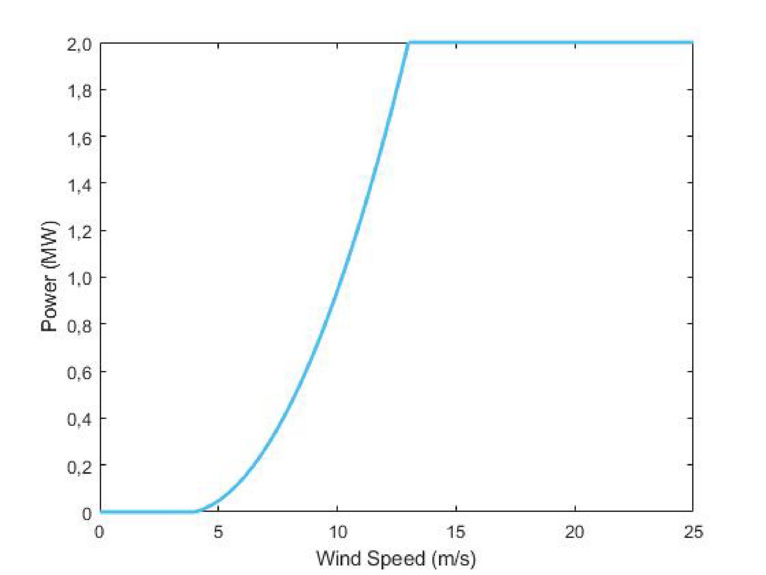
Figure 1 The power curve [15].

By limiting the ramp-rate of the power produced by the wind turbine we obtain a new power profile in which the steep rises and falls of power are smooth according to the limit chosen. We can clearly see this in Figure 2 where the difference in power production between the two cases is evident. In particular the production without limitation reaches about 0.4 MW around hour 15 and the limited production reaches about 0.15 MW at the same time.

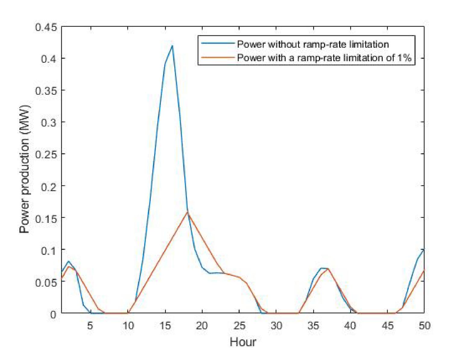
Figure 2 Comparison between power with and without a ramp-rate limitation of 1%.

In this work we consider the ramp-rate limitation of 1%, 2% and 5%. Furthermore, we consider the following two scenarios of battery configuration:

• 1-battery scenario in which we take into consideration only one battery connected to the system of capacity 0.36 MWh and with minimum and maximum SOC level equal to 0.036 MW and 0.324 MW, respectively.

• 2-battery scenario in which we take into consideration two batteries connected to the system of total capacity 0.72 MWh and with minimum and maximum SOC level equal to 0.036 MW and 0.648 MW, respectively.

In Table 1 and Table 2 mean, standard deviation, coefficient of Skewness and Kurtosis of the charge and discharge values, respectively, are shown. In particular, the real and the model statistics can be compared.

Table 1 Mean, standard deviation, coefficient of skewness and kurtosis of the charge values for the real and the modeled cases

Charge Values
Percentage limitation – Case	$Mean$	$Std$	$Skewness$	$kurtosis$
$1\%-Real$ $case$	0.4482	0.4401	1.0468	3.0908
$$
$1\%-Model$	0.4471	0.4401	1.0475	3.0788
$$
$2\%-Real$ $case$	0.3739	0.3721	1.2059	3.7162
$$
$2\%-Model$	0.3742	0.3728	1.2157	3.7356
$$
$5\%-Real$ $case$	0.2826	0.2887	1.4330	4.7442
$$
$5\%-Model$	0.2825	0.2868	1.4176	4.7106

Table 2 Mean, standard deviation, coefficient of skewness and kurtosis of the discharge values for the real and the modeled cases

Discharge Values
Percentage Limitation – Case	$Mean$	$Std$	$Skewness$	$kurtosis$
$1\%-Real$ $case$	-0.2562	0.2513	-1.4080	4.9237
$$
$1\%-Model$	-0.2559	0.2524	-1.4096	4.8816
$$
$2\%-Real$ $case$	-0.2943	0.2998	-1.4418	4.7503
$$
$2\%-Model$	-0.2939	0.2995	-1.4440	4.7737
$$
$5\%-Real$ $case$	-0.2759	0.2735	-1.4523	5.0271
$$
$5\%-Model$	-0.2751	0.2759	-1.4296	4.8188

As it is evident, the values of each statistics for real and modeled cases are similar both for the charge and discharge values.

We report the probability transition matrices for each ramp-rate limitation according to [15].

$\mathit{Matrix}(1\%)$	$=\left[\begin{array}{ccc}\hfill 0.889\hfill & \hfill 0.071\hfill & \hfill 0.039\hfill \\ \hfill 0.075\hfill & \hfill 0.817\hfill & \hfill 0.108\hfill \\ \hfill 0.060\hfill & \hfill 0.051\hfill & \hfill 0.889\hfill \end{array}\right]$	(66)
$\mathit{Matrix}(2\%)$	$=\left[\begin{array}{ccc}\hfill 0.859\hfill & \hfill 0.108\hfill & \hfill 0.033\hfill \\ \hfill 0.064\hfill & \hfill 0.855\hfill & \hfill 0.081\hfill \\ \hfill 0.055\hfill & \hfill 0.088\hfill & \hfill 0.858\hfill \end{array}\right]$	(67)
$\mathit{Matrix}(5\%)$	$=\left[\begin{array}{ccc}\hfill 0.788\hfill & \hfill 0.185\hfill & \hfill 0.027\hfill \\ \hfill 0.039\hfill & \hfill 0.917\hfill & \hfill 0.043\hfill \\ \hfill 0.039\hfill & \hfill 0.186\hfill & \hfill 0.775\hfill \end{array}\right]$	(68)

If we consider the matrix (67) which refers to the case of a ramp-rate percentage limitation equal to $2\%$ and we are in the status $-1$, we have the $86\%$ of probability that the next state is again $-1$.

Table 3 Real-case results of the average time measured in hours elapsed between fully charged and medium charged conditions, and fully charged and empty conditions

Battery Scenarios	1-battery	2-battery	1-battery	2-battery	1-battery	2-battery
Ramp-rate Limitation	$1\%$	$1\%$	$2\%$	$2\%$	$5\%$	$5\%$
$fully$ $charged-$	2.4228	3.3083	2.7337	4.4589	3.4168	4.8599
$half$ $charged$
$fully$ $charged-empty$	3.3043	4.6777	3.4342	4.8246	4.6058	6.4024

Table 4 Modeled results of the average time measured in hours elapsed between fully charged and medium charged conditions, and fully charged and empty conditions

Battery Scenarios	1-battery	2-battery	1-battery	2-battery	1-battery	2-battery
Ramp-rate Limitation	$1\%$	$1\%$	$2\%$	$2\%$	$5\%$	$5\%$
$fully$ $charged-$	1.3448	1.6721	1.4722	1.9659	2.0504	3.2790
$half$ $charged$
$fully$ $charged-empty$	2.2511	3.6150	2.3425	3.7199	3.2873	6.0083

In Tables 3 and 4 we show the results obtained from the real and the modeled cases, respectively. We considered the scenarios in which the battery switches from the fully charged condition to the half charged condition and from the fully charged condition to the empty condition. It is possible to notice that there is a growing trend of the amount of hours which follows both the increase of the ramp-rate percentage limitation and the increase of the capacity of the battery. The first aspect is due to the fact that a higher ramp-rate percentage corresponds to a less strict limitation and, consequently, to lower values of energy which have to be charged or discharged into/from the battery. The second aspect is a consequence of the bigger capacity available into the battery which can absorb more variations of power and spend more time to switch from the fully charged condition to the half charged or empty condition. What it is also evident, and corresponds to what we expect to happen, is that the average time to switch from the two extreme conditions of the battery is bigger than the one needed to reach the half charged condition.

4 Concluding Remarks

In this piece of work, we have proposed the computation of some hitting times for the SOC of a battery system connected to a wind power plant under a ramp-rate limitation scheme. The results consist in a system of integral equations expressing the first moment of the hitting times and to the proposal of a numerical discretization scheme that transforms the system of integral equations into a system of linear equations.

An application to a real wind speed data set is also presented as an illustration of the potentiality of the results. The theoretical results show a good agreement with those based on real data. This means that the model can be effectively applied in practical problems that the energy manager should face such as limitation of penalties for unavailability of battery power transmission or the optimal sizing of the storage system.

References

[1] G. F. Frate, L. Ferrari, and U. Desideri. Impact of Forecast Uncertainty on Wind Farm Profitability. Journal of Engineering for Gas Turbines and Power, 142(4), 2020.

[2] H. Dehghani, B. Vahidi, and S. H. Hosseinian. Wind farms participation in electricity markets considering uncertainties. Renewable Energy, 101:907–918, 2017.

[3] E. Hittinger, J. Apt, and J. F. Whitacre. The effect of variability-mitigating market rules on the operation of wind power plants. Energy Systems, 5(4):737–766, 2014.

[4] D. Lee, J. Kim, and R. Baldick. Ramp rates control of wind power output using a storage system and gaussian processes. University of Texas at Austin, Electrical and Computer Engineering, 2012.

[5] D. Lee and R. Baldick. Limiting ramp rate of wind power output using a battery based on the variance gamma process. In Conf. Renew. Energies Power, 1–6, 2012.

[6] E. Hittinger, J. F. Whitacre, and J. Apt. Compensating for wind variability using co-located natural gas generation and energy storage. Energy Systems, 1(4):417–439, 2010.

[7] S. Teleke, M. E. Baran, A. Q. Huang, S. Bhattacharya, and L. Anderson. Control strategies for battery energy storage for wind farm dispatching. IEEE Transactions on Energy Conversion, 24(3):725–732, 2009.

[8] Y. Uchida, G. Koshimizu, T. Nanahara, and K. Yoshimoto. New control method for regulating state-of-charge of a battery in hybrid wind power/battery energy storage system. In 2006 IEEE PES Power Systems Conference and Exposition, 1244–1251, 2006.

[9] F. Luo, K. Meng, Z. Y. Dong, Y. Zheng, Y. Chen, and K. P. Wong. Coordinated operational planning for wind farm with battery energy storage system. IEEE Transactions on Sustainable Energy, 6(1):253–262, 2015.

[10] D. L. Yao, S. S. Choi, K. J. Tseng, and T. T. Lie. Determination of short-term power dispatch schedule for a wind farm incorporated with dual-battery energy storage scheme. IEEE Transactions on Sustainable Energy, 3(1):74–84, 2011.

[11] A. Gautam, and S. Dharmaraja. An analytical model driven by fluid queue for battery life time of a user equipment in LTE-A networks. Physical Communication, 30:213–219, 2018.

[12] S. Kapoor, and S. Dharmaraja. Applications of Fluid Queues in Rechargeable Batteries. In Applied Probability and Stochastic Processes, 91–101, Springer, Singapore, 2020.

[13] G. D’Amico. Measuring the quality of life through Markov reward processes: analysis and inference. Environmetrics: The official journal of the International Environmetrics Society, 21(2):208–220, 2010.

[14] G. D’Amico, F. Gismondi, J. Janssen, and R. Manca. Discrete time homogeneous Markov processes for the study of the basic risk processes. Methodology and Computing in Applied Probability, 17(4):983–998, 2015.

[15] G. D’Amico, F. Petroni, and S. Vergine. An Analysis of a Storage System for a Wind Farm with Ramp-Rate Limitation. Energies, 14(13):4066, 2021.

[16] C. Venu, Y. Riffonneau, S. Bacha, and Y. Baghzouz. Battery storage system sizing in distribution feeders with distributed photovoltaic systems. In2009 IEEE Bucharest PowerTech, 1–5, 2009.

[17] Global Modeling and Assimilation Office (GMAO) (2015) Modern-Era Retrospective analysis for Research and Applications, Version 2. [https://gmao.gsfc.nasa.gov/reanalysis/MERRA-2/data_access/]. Accessed: [2021-07-15].

Biographies

Guglielmo D’Amico is a Full Professor in Mathematical Methods in Economics, Finance and Insurance at the Department of Economics of the “G. D’Annunzio” University of Chieti-Pescara. He received his PhD in Mathematics for applications in Economics, Finance and Insurance from the University “La Sapienza” of Rome in May 2005. His research interests include the theory of stochastic processes and their applications in finance, insurance, economics, reliability and wind energy. He is interested also in nonparametric statistical inference for stochastic processes. His research has appeared in several refereed journals: European Journal of Operational Research, Applied Mathematical Finance, Scandinavian Actuarial Journal, Applied Mathematical Modelling, IMA Journal of Management Mathematics, Journal of the Operational Research Society, Reliability Engineering and System Safety, Stochastics, Insurance: Mathematics and Economics.

Fulvio Gismondi is a Full Professor in Mathematical Methods in Economics, Finance and Insurance at the Department of Economic and Business Science at the “G. Marconi” University of Rome. He received his PhD in Actuarial Sciences from the University “La Sapienza” of Rome. His research interests include the theory of stochastic processes and their applications in finance and insurance. His research has appeared in several refereed journals: Methodology and Computing in Applied Probability, Mathematics, Physica a: Statistical Mechanics and its Applications, Theory of Probability and Mathematical Statistics, Annals of Actuarial Science.

Salvatore Vergine is a PhD student at the Department of Neurosciences, Imaging and Clinical Sciences of the “G. D’Annunzio” University of Chieti-Pescara. Before starting the university studies, he worked as a bank employee for two years. He gained his first Master’s degree in Civil Engineering at University of Salento in Apulia in April 2017. Afterwards, he got the Master’s degree in Environmental Engineering at Imperial College London in November 2020. His research interests focus on financial mathematics, stochastic processes, renewable energies and specifically wind energy. His first research has appeared in the journal Energies.

Journal of Reliability and Statistical Studies, Vol. 15, Issue 2 (2022), 431–458.
doi: 10.13052/jrss0974-8024.1522
© 2022 River Publishers