A Software Reliability Model Using Fault Removal Efficiency

Md. Asraful Haque^* and Nesar Ahmad

Department of Computer Engineering, Z.H. College of Engineering & Technology, Aligarh Muslim University, Aligarh-202002, India
E-mail: md_asraf@zhcet.ac.in; nesar.ahmad@gmail.com
*Corresponding Author

Received 28 December 2021; Accepted 01 May 2022; Publication 22 July 2022

Abstract

With the increase of human dependency over computer software, considerable effort has been given to determine software reliability effectively. A huge variety of software reliability growth models (SRGMs) have been developed to explain statistically how system reliability varies over time by monitoring the failure data sets during the testing process. The paper proposes a new SRGM based on taking into account the fault removal efficiency which is the ratio of corrected and detected faults during the testing process. The new model is compared to some known model from the relevant literature for two certain data sets and it turns out to perform better in terms of four GOF benchmarks.

Keywords: Reliability model, NHPP model, SRGM, software reliability engineering, project management.

1 Introduction

The word — “Reliability” is somehow a qualitative term. In general, a product is reliable, if it delivers on its promises. Most engineering products are expected to function reliably once they have been developed, tested, and delivered. Software industry suffers many challenges in producing highly reliable software. A software development project cannot go off the rails; the project manager must adhere to a strict timeline and budget. On the one hand, management expects its testing team to eliminate all software flaws in order to increase software reliability. The management, on the other hand, wants to keep testing expenses to a minimum. These are two characteristics of software development that cannot be overlooked. As a result, management must make an informed decision about when the software will be released. Early release may result in less reliable software but lower testing expenses. A later release would result in more reliable software, but at the expense of increased testing expenditures. In such a scenario, the management prefers an optimal path or a trade-off option based on the considerations of reliability growth and testing cost. The primary objective of employing SRGMs is to test and debug the system until it achieves the necessary level of reliability. An SRGM is a statistical model that forecasts how software reliability will increase over time when faults are found and fixed [1, 2]. The strategy is based on the notion that a program has faults and these faults present themselves as visible failures during the testing process, which are identified and corrected. A crucial component of the development of these statistical models is recognizing realistic assumptions and then modelling the testing activities effectively within a specified or adequate analytical framework. Software reliability models offer a systematic and quantitative approach to figure out the failures in a timely manner. These models aid management in determining the amount of time and effort that should be spent on testing [3]. Since 1970s, a plenty of SRGMs have been developed under various sets of assumptions on testing environment [4]. The majority of the models have a common drawback that is unrealistic assumptions. They assume that the faults are independent and that the faults are corrected as soon as they are identified i.e. the number of detected faults is equal to the number of corrected faults [5]. These two assumptions do not hold true in a real-world testing scenario. The remedy of one fault may be contingent on the correction of another fault in the future. As a result, it is not always possible to remove all the identified faults immediately. Furthermore, it’s possible that when fixing the target fault, some other faults are rectified as well, which may have been exposed in the future. It indirectly implies that detecting one fault leads to the correction of multiple faults. Thus, the number of repaired faults may be the same, higher, or lower than the number of detected faults in practise.

This paper presents a software reliability model that takes into account a special parameter “$\phi$” called fault removal efficiency that maps between the number of identified faults and the number of repaired faults. The fault removal efficiency is defined as the fault removal rate per detected fault.

2 Related Work

The most commonly used technique in developing the SRGMs is Non-homogeneous Poisson process (NHPP) [5]. Other techniques include Bayesian models, Markov models etc. Many recent models [6–11] emphasize the use of different machine learning methods including neural network, fuzzy logic, deep learning etc. The Jelinski-Mornada model [12], regarded as the first SRGM was published in 1972. Since then, a lot of work has been done as the researchers shown a great interest in suggesting novel models that would best suit the failure data from the past. The literature on reliability modelling is large and extensive, as many researchers came up with a variety of models based on a variety of assumptions and techniques. Goel and Okumoto [13] developed a simple NHPP model that received a huge attention by the researchers. The Delayed S-Shaped model [14] is a variant of the NHPP process that divides the testing process into two different phases: fault detection phase and fault removal phase. The model incorporates a learning process as a result of the project team’s increasing experience and skill improvement. The Inflection S-Shaped model [15] is developed under the assumption that some faults are not exposed before some others are removed. The likelihood of detecting a failure at any given time is related to the number of detectable defects in the program at the time. Kapur and Garg [16] suggested a model based on the concept of dependent faults. While correcting the leading faults, several additional faults (called dependent faults) that may have caused future failure are also corrected. Kapur et al. [17] also presented two general frameworks for NHPP models: one for when the fault detection and fault elimination processes are supposed to be the same, and another for when they are supposed to be separate processes. Huang et al. [18] proposed a model for software reliability growth that integrates fault dependency and a time-dependent delay function. Peng et al. [19] designed a model that includes the fault detection and fault removal processes with the presence of a testing effort function. Zhu and Pham [6] presented a software reliability model that took into account the fault-dependent detection and the imperfect fault removal. They used a genetic algorithm (GA) to estimate parameters in their model. Haque and Ahmad [20] proposed a similar type model that considers the issue of dependent faults in imperfect debugging environment. Haque and Ahmad [21] suggested another model that takes into account the uncertainty impact of the testing environment and assumptions when estimating software product reliability. Li and Pham [22] developed a model that uses fault introduction rate (i.e. number of new faults introduced per corrected fault) to represent the dependencies between fault detection and fault correction processes. The model additionally includes a testing coverage rate function. Chatterjee et al. [23] proposed a model that addresses the fault dependency issue in the context of multi-release software.

There are already a vast number of SRGMs, and it is impossible to include them all. We have tried to cover some models that address the issue of fault dependency. They are mainly based on imperfect debugging which provides the concept of fault introduction rate. These models simply consider $\phi <1$. There is one model known as Kapur-Garg model [16] that assumes $\phi >1$. However, most of the current SRGMs are based on the consideration that $\phi =1$. Our proposed model treats the fault detection and fault removal operations as two distinct processes and attempts to construct a link between them. The model is flexible to deal with any real value of $\phi$ (i.e. $\phi <1$, $\phi >1$ and $\phi =1$).

3 Proposed Model

The proposed model is an NHPP model that is represented using a mean value function. Most of the SRGMs suggested till now are based on the assumptions that the faults are independent and they are fixed as soon as they are detected (i.e. the number of detected faults are equal to the number of corrected faults). They use a generalized function [17, 24]:

$$\frac{\mathrm{dm}(\mathrm{t})}{\mathrm{dt}}=\mathrm{b}(\mathrm{t})[N-\mathrm{m}(\mathrm{t})]$$

(1)

where,

– m(t): estimated number of faults identified over time t.

– N: the total number of faults in the system before testing begins.

– b(t): time dependent fault detection rate function.

The proposed model uses the concept of fault removal efficiency by incorporating a parameter ‘$\phi$’. It is the ratio of corrected and detected faults. Naturally, $\phi \ge 0$. Here, $\phi <1$ means that the number of corrected faults is less than the number of detected faults and $\phi >1$ means that the number of corrected faults is greater than the number of detected faults. $\phi =1$ indicates that both are equal. Thus, the number of faults removed over time t is “$\phi \mathrm{m}(\mathrm{t})$” and Equation (1) can be framed as:

$$\frac{\mathrm{dm}(\mathrm{t})}{\mathrm{dt}}=\mathrm{b}(\mathrm{t})[\mathrm{N}-\phi \mathrm{m}\left(\mathrm{t}\right)]$$

(2)

In this paper, we use the two-parameter logistic function to represent the fault detection rate. It is generally known as the inflection S-shaped fault detection rate function which has been used in many studies [14, 25]. It is expressed as follows:

$$\mathrm{b}(\mathrm{t})=\frac{\mathrm{b}}{1+\beta {\mathrm{e}}^{-\mathrm{bt}}},\mathrm{b}>0,\beta >0;$$

(3)

where ‘b’ is a constant and $\beta$ is the inflection factor. Replacing the value of b(t) in Equation (2),

$$\frac{\mathrm{dm}(\mathrm{t})}{\mathrm{dt}}=\frac{\mathrm{b}}{1+\beta {\mathrm{e}}^{-\mathrm{bt}}}[\mathrm{N}-\phi \mathrm{m}\left(\mathrm{t}\right)]$$

(4)

Before testing begins, the number of detected faults and the number of corrected faults are both zero. Thus, $\phi =1$. Solving Equation (4), for the mean value function m(t) with these initial conditions (i.e. m(0) = 0 and $\phi =1$), we find:

$$\mathrm{m}(\mathrm{t})=\frac{\mathrm{N}}{\phi }\left[1-\frac{1+\beta }{{\left(\beta +{\mathrm{e}}^{\mathrm{bt}}\right)}^{\phi }}\right]$$

(5)

Table 1 presents the proposed model and some established models with their mean value functions.

Table 1 A set of reliability models

Model	m(t)
G-O Model [13]	a(1-${\mathrm{e}}^{-\mathrm{bt}}$)
DSS Model [14]	a(1-$(1+\mathrm{bt}){\mathrm{e}}^{\mathrm{bt}}$)
ISS Model [15]	${\displaystyle \frac{\mathrm{a}\left(1-{\mathrm{e}}^{-\mathrm{bt}}\right)}{1+\beta {\mathrm{e}}^{-\mathrm{bt}}}}$
TC Model [26]	$\mathrm{N}\left(1-{\left({\displaystyle \frac{\beta }{\beta +{\left(\mathrm{at}\right)}^{\mathrm{b}}}}\right)}^{\alpha }\right)$
Loglog Model [27]	N(1$-{\mathrm{e}}^{-({\mathrm{a}}^{{\mathrm{t}}^{\mathrm{b}}}-1)}$)
New Model	${\displaystyle \frac{\mathrm{N}}{\phi }}\left[1-{\displaystyle \frac{1+\beta }{{\left(\beta +{\mathrm{e}}^{\mathrm{bt}}\right)}^{\phi }}}\right]$

4 Model Validation, Comparison and Analysis

The acceptability of a model is determined by identifying its strengths, weaknesses, and the level of trust that can be placed in the findings presented. SRGMs are evaluated using two major steps: first, parameter estimation and second, verification of the model fittings using different comparison criteria. The performance analysis of the new model is discussed in detail in the following subsections. The model was compared to some existing models mentioned in Table 1.

4.1 Comparison Criteria

An SRGM is judged based on its potential to recreate the software’s actual behaviour and forecast the software’s future behaviour using past failure data. There are many Goodness-of-Fit (GOF) criteria available to compare the efficiency of different models and investigate how well a model fits a set of observations. In this paper, the model validation has been carried out using four GOF criteria namely – Mean square error or MSE, Predictive ratio risk or PRR, Coefficient of determination or R${}^2$ and Akaike information criteria or AIC. The formulas of these criteria [21, 28] are given below where, ‘n’ denotes the number of samples in the dataset, and ‘p’ denotes the number of model parameters.

• MSE: The mean square error (MSE) represents the average squared residual (i.e. the difference between the observed value and predicted value), and is defined as:

$$\mathrm{MSE}=\frac{\sum _{\mathrm{i}=1}^{\mathrm{n}}{({\mathrm{m}}_{\mathrm{i}}-\mathrm{m}({\mathrm{t}}_{\mathrm{i}}))}^2}{\mathrm{n}-\mathrm{p}}$$

• PRR: The predictive-ratio risk (PRR) calculates the error per model-estimate and it is defined as:

$$\mathrm{PRR}=\sum _{\mathrm{i}=1}^{\mathrm{n}}{\left(\frac{\mathrm{m}({\mathrm{t}}_{\mathrm{i}})-{\mathrm{m}}_{\mathrm{i}}}{\mathrm{m}({\mathrm{t}}_{\mathrm{i}})}\right)}^2$$

• R${}^{\mathrm{2}}$: It measures the distribution of data points around the fitted regression line. This evaluation criteria is also known as the coefficient of determination:

$${\mathrm{R}}^2=1-\frac{\sum _{\mathrm{i}=1}^{\mathrm{n}}{({\mathrm{m}}_{\mathrm{i}}-\mathrm{m}({\mathrm{t}}_{\mathrm{i}}))}^2}{\sum _{\mathrm{i}=1}^{\mathrm{n}}{({\mathrm{m}}_{\mathrm{i}}-\sum _{\mathrm{j}=1}^{\mathrm{n}}\frac{{\mathrm{m}}_{\mathrm{j}}}{\mathrm{n}})}^2}$$

• AIC: AIC is used to determine which of several models is most likely to be the best for a given dataset by providing a score value that penalizes the number of model parameters. The well known formula of AIC is:

$$\mathrm{AIC}=2\mathrm{p}-2\log (\mathrm{L})$$

where, L represents the maximum likelihood estimate. An alternate measure for LSE regression is as follows [29]:

$$\mathrm{AIC}=\mathrm{n}\times \ln \left(\mathrm{MSE}\right)+2\mathrm{p}$$

The smaller MSE, PRR, and AIC values, as well as the greater R${}^2$ value that tends to 1, are always anticipated to justify fewer fitting flaws and improved model performance [27].

4.2 Dataset Used

In [30], the failure datasets of four different releases of a Tandem Computer Project have been reported. We used the failure data of first two releases for our model validation and comparison. In release-1, after 20 weeks of testing and 10000 hrs of CPU execution, total 100 errors were collected. In release-2, total 120 errors were reported over the testing duration of 19 weeks and 10272 CPU Hrs. The datasets of Release-1 and Release-2 are shown together in Table 2.

Table 2 Tandem computers test data

	Cumulative Faults		Cumulative Faults
Test Week	Release-1	Release-2	Test Week	Release-1	Release-2
1	16	13	11	81	95
2	24	18	12	86	100
3	27	26	13	90	104
4	33	34	14	93	110
5	41	40	15	96	112
6	49	48	16	98	114
7	54	61	17	99	117
8	58	75	18	100	118
9	69	84	19	100	120
10	75	89	20	100	—

4.3 Results and Comparison

The fittings of software reliability models are determined only when it is feasible to estimate their parameters. Parameter estimation refers to the process of making efficient use of sample data in estimating the values of unknown variables that exist in the mathematical models [31]. There are several techniques available to estimate the parameters, for example, least square estimation, maximum likelihood estimation, Bayes parameter estimation etc. Generally, LSE is recommended when the sample size is small and censoring is not particularly heavy [32, 33]. Thus, we have preferred Least Square Estimation (LSE) approach to decide the parameters’ values of all six models (listed in Table 1).

Then we can calculate the aforementioned four GOF criteria of all SRGMs using the parameter values. For the Tandem project release-1 dataset, Table 3 provides the results including the estimated parameter values and criteria values. Similarly, Table 4 presents the results for release-2 dataset. The following is a summary of the Table 3:

• MSE $=$ 1.936. It is nearly four times lower than the second best value achieved (i.e. Loglog model – 8.437) in this study.

• PRR= 0.026. It is roughly 8-times lower than the second best value for G-O model.

• R${}^2$ $=$ 0.998. It is the highest among all models.

• AIC $=$ 10.751 which is the smallest among all models.

Table 3 Model validation on release-1 dataset

Model	LSEs	MSE	PRR	R${}^2$	AIC
G-O Model	a $=$ 130.2, b $=$ 0.083	12.915	0.203	0.986	51.061
DSS Model	a $=$ 103.984, b $=$ 0.265	28.066	1.084	0.969	66.584
ISS Model	a $=$ 110.829, b $=$ 0.172, $\beta$ $=$ 1.205	10.564	0.305	0.989	47.899
TC Model	N $=$ 119.205, a $=$ 13.798$\times$10${}^{-3}$, b $=$ 1.111, $\beta$ $=$ 7.337, $\alpha$ $=$ 65.069	14.577	0.3	0.987	55.836
Loglog Model	N $=$ 105.109, a $=$ 1.095, b $=$ 0.947	8.437	0.238	0.991	43.403
New Model	N $=$ 110.382, b $=$ 0.287, $\beta$ $=$ 7.624, $\phi$ $=$ 1.069	1.936	0.026	0.998	10.751

Table 4 Model validation on release-2 dataset

Model	LSEs	MSE	PRR	R${}^2$	AIC
G-O Model	a $=$ 182.95, b $=$ 0.061	26.217	0.212	0.982	59.948
DSS Model	a $=$ 127.399, b $=$ 0.242	14.693	0.796	0.990	48.946
ISS Model	a $=$ 124.445, b $=$ 0.254, $\beta$ $=$ 3.778	7.139	0.261	0.996	35.08
TC Model	N $=$ 128.17, a $=$ 0.02, b $=$ 1.442, $\beta$ $=$ 7.05, $\alpha$ $=$ 83.734.	12.913	0.45	0.993	45.805
Loglog Model	N $=$ 119.881, a $=$ 1.06, b $=$ 1.157	7.956	0.263	0.995	37.139
New Model	N $=$ 124.553, b $=$ 0.314, $\beta$ $=$ 8.258, $\phi$ $=$ 1.032	3.77	0.016	0.998	22.724

Table 4 can be summarized as:

• MSE $=$ 3.77. It is near about half of the second best value achieved (i.e. ISS model – 7.139) in this study.

• PRR $=$ 0.016. It is nearly 13-times lower than the second best value achieved (i.e. 0.212) in this study.

• R${}^2$ $=$ 0.998 again. It is the highest among all models.

• AIC $=$ 22.724 which is the smallest among all models.

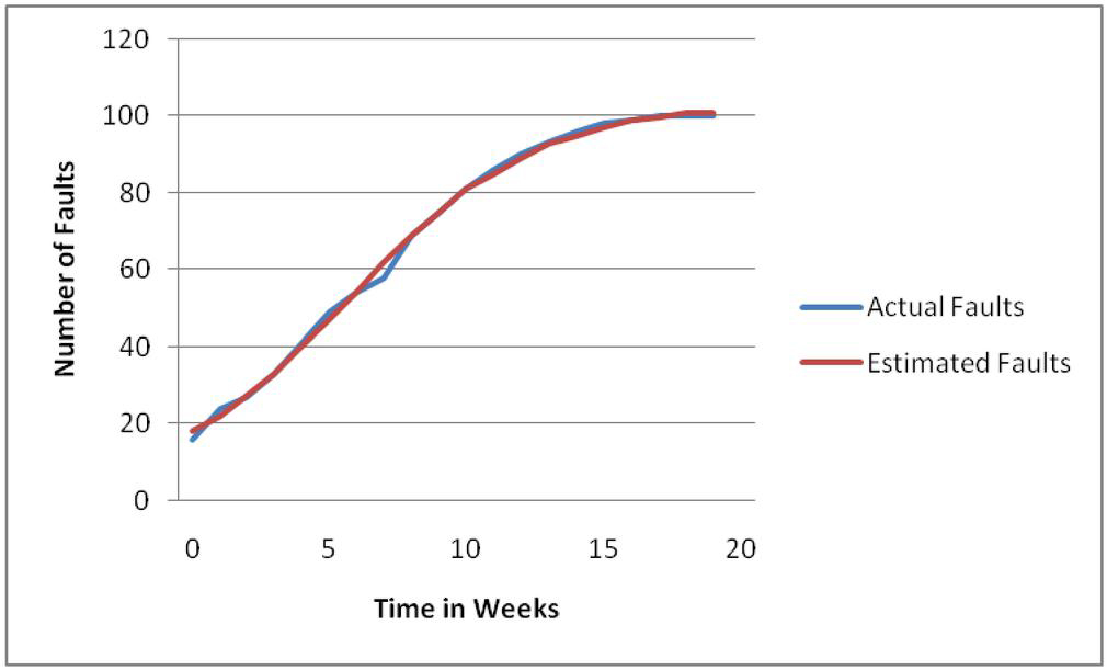
Figure 1 Model performance on release-1 dataset.

Thus on both the datasets, the proposed model achieved the best fitting values with the lowest MSE, PRR, AIC and the highest R${}^2$. Figures 1 and 2 display the curves representing the model performance on each dataset, comparing the estimated faults to the observed faults.

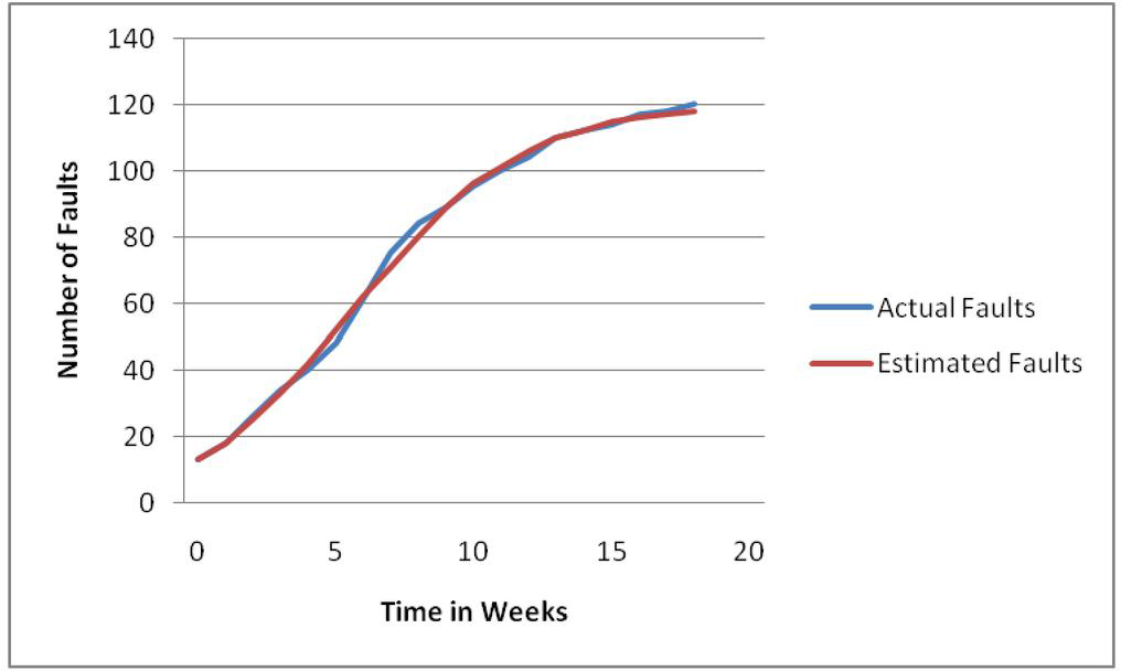
Figure 2 Model performance on release-2 dataset.

5 Conclusion

The new model suggested in the paper, establishes a relationship between fault detection and fault correction processes assuming that they are two different processes. It incorporates the widely used inflection S-shaped fault detection rate function and a parameter that represents the fault removal efficiency. The model has been validated on two real world datasets and compared its Goodness-of-fit with five reputed models using four evaluation criteria. In all four benchmarks, the findings clearly indicate that the proposed model beats the other five models. The accuracy of SRGMs heavily depends on the types of datasets. A model may perform well on some datasets while failing to deliver good results on others. Therefore, it will be premature to claim the superiority of the model. In the future, we will concentrate on a thorough analysis of the model using a wide range of datasets and other comparison criteria.

References

[1] R. Lai, M. Garg, “A Detailed Study of NHPP Software Reliability Models”, Journal of Software, Vol. 7, No. 6, pp. 1296–1306, June 2012.

[2] MA Haque and N. Ahmad, “An Effective Software Reliability Growth Model”, Safety and Reliability, 2021, vol. 40, Issue-4, pp. 209–220.

[3] C. J. Hsu, C. Y. Huang and J. R. Chang, Enhancing software reliability modeling and prediction through the introduction of time-variable fault reduction factor, Appl. Math. Model. 35(1) (2011) 506–521.

[4] M. A. Haque and N. Ahmad, “An Imperfect SRGM based on NHPP,” 2021 Third International Conference on Inventive Research in Computing Applications (ICIRCA), 2021, pp. 1574–1577.

[5] M. Zhu, H. Pham, “A software reliability model with time-dependent fault detection and fault removal”, Vietnam Journal of Computer Science 3, pp. 71–79, 2016.

[6] S. Ramasamy and I. Lakshmanan, “Machine Learning Approach for Software Reliability Growth Modeling with Infinite Testing Effort Function”, Mathematical Problems in Engineering, vol. 2017, Article ID 8040346, 6 pages, 2017.

[7] SWA Rizvi, VK Singh and RA Khan, “Fuzzy Logic Based Software Reliability Quantification Framework: Early Stage Perspective (FLSRQF)”, Procedia Computer Science, volume 89, pages 359–368, 2016.

[8] J. Wang, C. Zhang, “Software reliability prediction using a deep learning model based on the RNN encoder-decoder”, Reliability Engineering & System Safety, vol. 170, pp. 73–82, 2018.

[9] Y. Tamura, S. Yamada, “Software Reliability Model Selection Based on Deep Learning with Application to the Optimal Release Problem”, Journal of Industrial Engg. & Mgmt. Science, 2016, Article no. 3, pp. 43–58.

[10] Y. Minamino, S. Inoue, S. Yamada, “Change-Point–Based Software Reliability Modeling and Its Application for Software Development Management”, In Recent Advancements in Software Reliability Assurance; CRC Press: Boca Raton, FL, USA, 2019; pp. 59–92.

[11] A. Jaiswal and R. Malhotra, “Software reliability prediction using machine learning techniques”, Int J. of System Assurance Engineering and Management 9, pp. 230–244, 2018.

[12] Z. Jelinski, P. B. Moranda, “Software reliability research”, in Statistical Computer Performance Evaluation, Freiberger W. (ed.), Academic Press, New York, pp. 465–484, 1972.

[13] A. L. Goel, K. Okumoto, “Time-Dependent Error-Detection Rate Model for Software Reliability and Other Performance Measures,” in IEEE Transactions on Reliability, vol. R-28, no. 3, pp. 206–211, 1979.

[14] S. Yamada, M. Ohba and S. Osaki, “s-Shaped Software Reliability Growth Models and Their Applications,” in IEEE Transactions on Reliability, vol. R-33, no. 4, pp. 289–292, Oct. 1984.

[15] M. Ohba, “Inflection S-Shaped Software Reliability Growth Model”, In: Osaki S., Hatoyama Y. (eds) Stochastic Models in Reliability Theory. Lecture Notes in Economics and Mathematical Systems, vol. 235. Springer, Berlin, Heidelberg. 1984.

[16] P.K. Kapur and R.B. Garg, “A software reliability growth model for an error-removal phenomenon”, Software Engineering Journal, Volume 7, Issue 4, July 1992, pp. 291–294.

[17] P. K. Kapur, H. Pham, S. Anand, K. Yadav, “A Unified Approach for Developing Software Reliability Growth Models in the Presence of Imperfect Debugging and Error Generation”, in IEEE Transactions on Reliability, vol. 60, no. 1, pp. 331–340, 2011.

[18] Chin-Yu Huang, Chu-Ti Lin, Sy-Yen Kuo, M. R. Lyu and C. Sue, “Software reliability growth models incorporating fault dependency with various debugging time lags,” Proc. of the 28th Annual Int. Computer Software and Applications Conference, 2004. COMPSAC 2004, vol. 1, pp. 186–191.

[19] R. Peng et al., “Testing effort dependent software reliability model for imperfect debugging process considering both detection and correction”, Reliability Engineering & System Safety, Volume 126, 2014, Pages 37–43.

[20] MA Haque and N. Ahmad, “A software reliability growth model considering mutual fault dependency”, Reliability: Theory and Applications, 2021, 16(2), pp. 222–229.

[21] MA Haque and N. Ahmad, “A Logistic Growth Model for Software Reliability Estimation Considering Uncertain Factors”, Int. Journal of Reliability, Quality and Safety Engineering, Vol. No. 28, Issue 05, Article No. 2150032, 2021.

[22] Q. Li, H. Pham, “Modeling Software Fault-Detection and Fault-Correction Processes by Considering the Dependencies between Fault Amounts. Appl. Sci. 2021, 11, 6998.

[23] S. Chatterjee, D. Saha, and A. Sharma, “Multi-upgradation software reliability growth model with dependency of faults under change point and imperfect debugging”, Journal of Software: Evolution and Process 33(6), 2021.

[24] KY Song, IH Chang, MS Choi. “A software reliability model with a Burr Type III fault detection rate function”, International Journal of Reliability and Applications 17.2 (2016): 149–158.

[25] H. Pham, “A Logistic Fault-Dependent Detection Software Reliability Model”, Journal of Universal Computer Science, vol. 24, no. 12 (2018), 1717–1730.

[26] I. H. Chang, H. Pham, S.W. Lee, K.Y. Song, “A testing-coverage software reliability model with the uncertainty of operation environments”, Int. J. of Systems Science: Operations & Logistics. 2014, 1(4), pp. 220–227.

[27] H. Pham, “Loglog fault-detection rate and testing coverage software reliability models subject to random environments”, Vietnam Journal of Computer Science 1(1), pp. 39–45, 2014.

[28] M. A. Haque and N. Ahmad, “An NHPP-Based SRGM with Time Dependent Growth Process,” 2021 6th International Conference on Signal Processing, Computing and Control (ISPCC), 2021, pp. 155–158.

[29] Akaike information criterion: https://en.wikipedia.org/wiki/Akaike\_information\_criterion

[30] A. Wood, “Software reliability growth models”, In Tandem Technical Report-96.1, 1996.

[31] J V Beck and K J Arnold, “Parameter estimation in engineering and science”, Wiley series in probability and mathematical statistics, Wiley Publisher, New York, 1977.

[32] C. Wohlin, “Estimation of Software Reliability Growth Model Parameters”, Proceedings of Workshop on Reliability Analysis of System Failure Data, Microsoft Research, 2007 Cambridge, UK.

[33] M. A. Haque and N. Ahmad, “Key Issues in Software Reliability Growth Models”, Recent Advances in Computer Science and Communications 2022; Vol. 15, Issue 5, pp. 741–747.

Biographies

Md. Asraful Haque, Assistant Professor in Zakir Hussain College of Engineering & Technology currently pursuing his Ph.D. in the field of Software Engineering from AMU. He has more than 12 years of teaching experience. He received his B.Tech degree in 2007 and M.Tech degree in 2012. His area of interests includes Software engineering, Operating Systems, Data Structure, Database Management Systems etc.

Nesar Ahmad received B.Sc (Engg) degree from Bihar College of Engineering, Patna (Now NIT, Patna) in 1984. He received M.Sc (Information Engineering) degree from City University, London, U.K., in 1988, and Ph.D degree from IIT, Delhi, in 1993. He is currently a Professor in the Department of Computer Engineering, Aligarh Mulsim University, Aligarh. His current research interests mainly include Artificial Intelligence, Applied Soft Computing, and Digital Learning.

Journal of Reliability and Statistical Studies, Vol. 15, Issue 2 (2022), 459–472.
doi: 10.13052/jrss0974-8024.1523
© 2022 River Publishers

Abstract

1 Introduction

2 Related Work

3 Proposed Model

4 Model Validation, Comparison and Analysis

4.1 Comparison Criteria

4.2 Dataset Used

4.3 Results and Comparison

5 Conclusion

References

Biographies