Classical and Bayesian Inference for the Inverse Lomax Distribution Under Adaptive Progressive Type-II Censored Data with COVID-19 Application

Rashi Hora¹, Naresh Chandra Kabdwal¹ and Pulkit Srivastava^2,*

¹Department of Mathematics and Statistics, Banasthali Vidyapith, Tonk, Rajasthan, 304022, India
²Department of Statistics, University of Delhi, Delhi, 110007, India
E-mail: horarashi@gmail.com; kabdwal.dr@gmail.com; pulkit.stats@gmail.com
*Corresponding Author

Received 30 January 2022; Accepted 30 May 2022; Publication 22 July 2022

Abstract

In this paper, we consider the classical and the Bayesian inferences for unknown parameters of inverse Lomax distribution and their corresponding survival characteristics under the adaptive progressive type-II censoring scheme. In the classical setup, first we obtain the maximum likelihood estimates for the unknown shape parameter of the distribution and its corresponding survival characteristics. Further, we consider symmetric and asymmetric loss functions for the estimation of shape parameter and its corresponding survival characteristics under the Bayesian paradigm. The performances of various derived estimators were recorded using Markov chain Monte Carlo simulation technique for different sample sizes. Finally, a COVID-19 mortality data set is provided to illustrate the computation of various estimators.

Keywords: Inverse Lomax distribution, adaptive progressive type-II censoring, maximum likelihood estimator, Bayesian estimation, Markov chain Monte Carlo, COVID-19.

1 Introduction

Several life-time models are available in literatures which play an extensive role to analyse the uncertainty of various fields. Initially, exponential distribution was very famous and useful because of its simplicity and analytical flexibility. Although, the exponential distribution has limitations in the study of life-time models due to its constant hazard rate, which is not appropriate to analyse many life-time models. Therefore, several other researchers have proposed different new life-time distributions which overcome the limitation of constant hazard rate. Such few specific distributions are Weibull distribution, gamma distribution, Lomax distribution, lognormal distribution which are extension of exponential distribution. The Lomax or Pareto II distribution as non-constant hazard rate distribution was proposed by Lomax (1954) [28]. Ahsanullah (1991) [2], Balakrishnan and Ahsanullah (1994) [7] and Lee et al. (2009) [27] discussed the properties and moments of Lomax distribution. Kleiber and Kotz (2003) [25] discussed inverse Lomax distribution (ILD) in the fields of stochastic modelling, actuarial sciences, economics and life testing. The ILD was used by Kleiber (2004) [24] to obtain Lorenz ordering relationship among ordered statistics. This distribution is a special case of generalized beta distribution of second kind and the said distribution also belongs to an inverted family of distribution. It has analytical flexibility where the non-monotonicity of failure rate has been realized (see, Singh et al (2013) [37]). Rehman et al. (2013) [33] discussed the problem of estimation and prediction for ILD through Bayesian approach. The survival estimation under type-II censoring scheme and the Bayesian estimation under type-II hybrid censoring scheme for this distribution were discussed by Singh et al. (2016) [38] and Yadav et al. (2016) [44] respectively. Jan and Ahmad (2017) [23] used approximation techniques through Bayesian approach. Recently, Sharma and Kumar (2020) [36] discussed the problem of parameter estimation under type-II censoring scheme for ILD.

The probability density function (PDF) $f(x)$ and Cumulative distribution function (CDF) $F(x)$ of the ILD with shape parameter $\alpha$ and scale parameter $\beta$ are given by

$$f(x;\alpha ,\beta )=\frac{\alpha \beta }{x^2}{\left(1+\frac{\beta }{x}\right)}^{-\left(1+\alpha \right)},x>0,\alpha ,\beta >0$$

(1)

and

$$F(x)={\left(1+\frac{\beta }{x}\right)}^{-\alpha }$$

(2)

The corresponding survival function $S(t)$ and hazard function $H(t)$ of this distribution at same time $t>0$ are given, respectively, by

$$S(t)=1-{\left(1+\frac{\beta }{t}\right)}^{-\alpha }$$

(3)

and

$$H(t)=\frac{\alpha \beta {\left(1+\frac{\beta }{t}\right)}^{-(1+\alpha )}}{t^2{\left(1+\frac{\beta }{t}\right)}^{-\alpha }}$$

(4)

In any life-testing experiments, it is very cumbersome to complete the experiment for a long period due to time and cost constraints. There are various types of censoring schemes which have been introduced in the literature to reduce the time and cost involved into the experiments. Among the various schemes, Type-I censoring and Type-II censoring are the two most common censoring schemes. In Type-I censoring, the life testing experiment is terminated at a pre-determined time whereas in Type-II censoring, lifetime experiment terminates after achieving a certain number of failures. These two are the most commonly used censoring schemes but these both schemes don’t have the flexibility of removing the units from the experiment. Progressive censoring scheme proposed by Cohen (1963) [15]. In this scheme, the experimenter initially puts $n$ units, $X_1,X_2,\mathrm{\dots }{X}_n$, at time zero and the test can be terminated at the time of any failure. When the first failure has occurred, $r_1$ of the remaining $(n-1)$ surviving units are removed randomly from the experiment. At the time of the second failure $r_2$ of the remaining $n-r_1-2$ surviving units are chosen randomly and removed from the experiment. At the time of $m^{th}$ observed failure, the experiment eventually terminates with removals of all remaining $r_m=n-r_1-r_2-\mathrm{\cdots }-m$ surviving units. In this scheme, $r_i$ and $m$ are fixed in advance. A more general censoring scheme, called type-II progressive censoring was introduced. In progressive type-II censoring scheme, the experimenter may not change the experiment time accordingly under the experiment. Thus, Ng et al. (2009) [32] suggested an adaptive progressive type-II (APT-II) censoring scheme which is the mixture of type I and progressive type-II censoring scheme. In APT-II censoring scheme, the total test time $T$ and the number of observed failure $m$ is prefixed i.e. $X_m<T$. Suppose the number of failure $j$ is observed before time $T$ i.e. $X_j<T<X_{j+1}$, $j=0,1,\mathrm{\dots },m$ where $X_0=0$ and $X_{m+1}=\mathrm{\infty }$. If the experimenter time runs over $T$, then set $R_{j+1}=\mathrm{\cdots }=R_m=0$. The pictorial representation of this scheme is given in Figure 1.

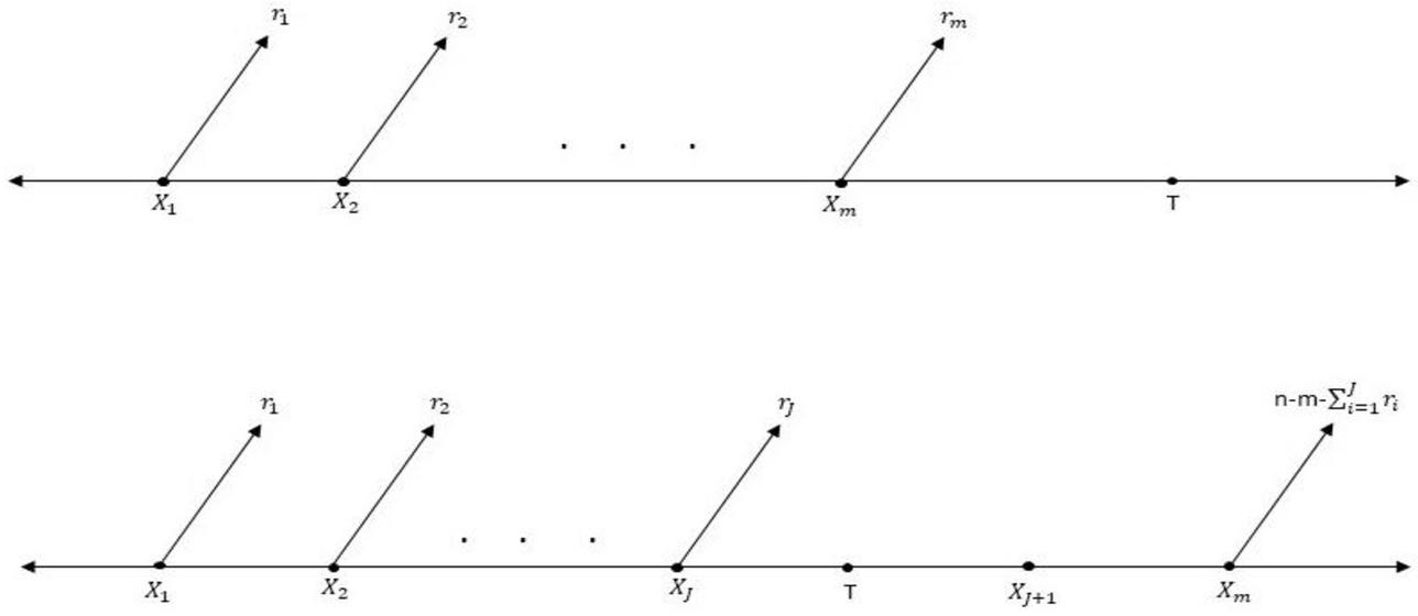
Figure 1 Schematic representation of Adaptive progressive type-II censoring scheme.

This censoring scheme has been considered by many researchers for statistical analysis on different lifetime distributions. The statistical analysis under APT-II censoring scheme for exponential distribution was proposed by Ng et al. (2009) [32]. Parameter estimation of generalized Pareto distribution was discussed by Mahmoud et al. (2013) [29] for APT-II censored data. Ye et al. (2014) [45] and Sobhi and Soliman (2016) [40] considered extreme value distribution and exponential Weibull distribution respectively for parameter estimation under APT-II censoring scheme. The classical and Bayesian inference for a general exponential form of underlying distribution under APT-II censored data was discussed by El-Din et al. (2018) [18]. Almetwally et al. (2019) [5] considered the APT-II censoring scheme for the generalized Rayeigh distribution. El-Sagheer et al. (2019) [19] and Sewailem (2019) [35] studied APT-II censored data for statistical analysis of Weibull exponential and log-logistic distribution respectively. Recently, Mohan and Chacko (2021) [30] considered Kumarswamy-exponential distribution under APT-II censoring scheme.

The present paper considers the problem of estimating shape parameter and survival characteristics of ILD under APT-II censoring scheme when scale parameter is known.

The rest of the paper is organized as follows. In Section 2, the Maximum likelihood estimation (MLE) for the shape parameter and the survival characteristics of ILD are presented. The Bayes estimation under symmetric and asymmetric loss functions are obtained in Section 3. Squared error loss function (SELF) is taken as symmetric loss function. General entropy loss function (GELF) and linear exponential loss function (LINEX) are taken as asymmetric loss function. In Section 4, interval estimation is described. Asymptotic confidence intervals (ACI) are obtained under classical set up. Credible interval and highest posterior density (HPD) intervals are constructed under Bayesian paradigm. In Section 5, Markov Chain Monte Carlo technique is discussed. A simulation study is presented to report the performances of the various estimators in Section 6. In Section 7, a COVID-19 mortality data set is provided to illustrate the computation of various estimators. Lastly, the conclusions appear in Section 8.

2 Maximum Likelihood Estimation

Suppose $n$ items are put on test from the ILD with pdf $f(x)$ and cdf $F(x)$ given in Equations (1) and (2) respectively. Let$X_{(1)}\le X_{(2)}\le X_{(3)}\le \mathrm{\cdots }\le X_{(m)},1\le m\le n$, be an APT-II censored sample with censoring scheme $(R_1,R_2,\mathrm{\dots },R_m)$. The likelihood function based on the APT-II censored sample is given by

$$l(\alpha ,\beta |\mathbf{x})={\mathrm{B}}_K\left(\prod _{i=1}^{m}f(x_i)\right){\left(\prod _{i=1}^K(1-F(x_i))\right)}^{r_i}{(1-F(x_m))}^{n-m-{\sum }_{i=1}^K{r}_i}$$

(5)

where,

$$B_K=\prod _{i=1}^m\left(n-i+1-\sum _{h=1}^{max(i-1,K)}{r}_h\right)$$

Substituting Equations (1) and (2) into Equation (5), the likelihood function will be

$l(\alpha ,\beta |\mathbf{x})$	$={\mathrm{B}}_K\left({\displaystyle \prod _{i=1}^m}{\displaystyle \frac{\alpha \beta }{x_i^2}}{\left(1+{\displaystyle \frac{\beta }{x_i}}\right)}^{-\left(1+\alpha \right)}\right)$
	$\mathrm{\hspace{1em}}\times {\left({\displaystyle \prod _{i=1}^K}\left(1-{\left(1+{\displaystyle \frac{\beta }{x_i}}\right)}^{-\alpha }\right)\right)}^{r_i}$
	$\mathrm{\hspace{1em}}\times {\left(1-{\left(1+{\displaystyle \frac{\beta }{x_m}}\right)}^{-\alpha }\right)}^{n-m-\sum _{i=1}^K{r}_i}$	(6)

The corresponding log-likelihood function can be written as

$L$	$=\ln l(\alpha ,\beta |\mathbf{x})$
	$=A+m\ln \alpha +mln\beta -{\displaystyle \sum _{i=1}^m}ln{x}_i-(1+\alpha ){\displaystyle \sum _{i=1}^m}\ln \left(1+{\displaystyle \frac{\beta }{x_i}}\right)$
	$\mathrm{\hspace{1em}}-\alpha {\displaystyle \sum _{i=1}^K}{r}_{i}ln\left(1+{\displaystyle \frac{\beta }{x_i}}\right)-\alpha \left(n-m-{\displaystyle \sum _{i=1}^K}{r}_i\right)ln\left(1+{\displaystyle \frac{\beta }{x_m}}\right)$

where, $A=ln{B}_K$.

Further, obtaining partial derivative of the Equation (2) with respect to parameter $\alpha$ and equating it to zero will give the normal equation to find the MLE of the unknown shape parameter as

${\displaystyle \frac{\partial L}{\partial \alpha }}$	$={\displaystyle \frac{m}{\alpha }}-{\displaystyle \sum _{i=1}^m}ln\left(1+{\displaystyle \frac{\beta }{x_i}}\right)+{\displaystyle \sum _{i=1}^K}{r}_{i}ln\left(1+{\displaystyle \frac{\beta }{x_i}}\right)$
	$\mathrm{\hspace{1em}}+\left(n-m-{\displaystyle \sum _{i=1}^K}{r}_i\right)\ln \left(1+{\displaystyle \frac{\beta }{x_m}}\right)$	(8)

From the Equation (2), it is clear that the normal equation does not yield the MLE of $\alpha$ because of its implicit form. Therefore, the MLE of the unknown shape parameter cannot be obtained analytically. Thus, one may use any numerical approximation techniques, such as, Newton-Raphson (N-R) method, fixed point iterations, etc. In this paper, we have used N-R method to evaluate the MLE of the parameters. Using the invariance property of MLE, expressions for the MLEs of survival characteristics are given as

$$\widehat{S(t)}=1-{\left(1+\frac{\beta }{t}\right)}^{-\widehat{\alpha }}$$

(9)

and

$$\widehat{H(t)}=\frac{\widehat{\alpha }\beta {\left(1+\frac{\beta }{t}\right)}^{-\left(1+\widehat{\alpha }\right)}}{t^2{\left(1+\frac{\beta }{t}\right)}^{-\widehat{\alpha }}}$$

(10)

3 Bayesian Estimation

In this section, we obtain Bayes estimates of unknown shape parameter of the distribution and survival characteristics of ILD under the symmetric and asymmetric loss functions. Most of the inferential procedures for lifetime models are frequently developed under the squared error loss function (SELF), which is symmetrical and associates equal importance to the losses due to overestimation and underestimation of equal magnitude. But in survival and hazard rate functions, the nature of losses are not always symmetric and hence the use of SELF is impractical in many situations. Inappropriateness of SELF has been recognized by different authors. Ferguson (1967) [20], Zellner and Geisel (1968) [46], Aitchison and Dunsmore (1975) [3], Varian (1975) [43] and Berger (1980) [10] are few among many authors. It is because of this fact that Varian (1975) [43] introduced LINEX loss function (LLF). But it has pointed out by various authors that LINEX loss function is not as appropriate for the estimation of the scale parameters. Keeping this point in mind, Basu and Ebrahimi (1991) [9] defined a modified LINEX loss function. A suitable alternative to the modified LINEX loss function is the general entropy loss function (GELF) proposed by Calabria and Pulcini (1996) [12]. Some works considers symmetric/asymmetric or both loss functions for parameter estimation in Bayesian inference (see, Soliman et al. (2013) [41], Goyal et al. (2019) [21] and Hora et al. (2021) [22], Albalawi et al. (2022) [4]).

When no information is given regarding parameter then non-informative prior is good choice. To incorporate some given previous information, informative prior has been used. The prior distribution for unknown shape parameter is thus taken to be Gamma distribution, i.e.,

$$\pi (\alpha )=\frac{a^b{\alpha }^{b-1}{e}^{-a\alpha }}{\mathrm{\Gamma }b},\alpha >0,a,b>0$$

(11)

where a and b are hyperparameters.

Combining the likelihood function and prior density using Bayes theorem, the posterior density is given as

$\mathrm{\Pi }(\alpha ,\beta |\mathbf{x})$	$={\displaystyle \frac{\pi \left(\alpha \right)l(\alpha ,\beta |\mathbf{x})}{{\int }_0^{\mathrm{\infty }}\pi (\alpha )l(\alpha ,\beta |\mathbf{x})\mathit{d}\alpha }}$
$\mathrm{\Pi }(\alpha ,\beta |\mathbf{x})$	$={\displaystyle \frac{K_1}{K_0}}$	(12)

where,

$K_1$	$=\left({\displaystyle \prod _{i=1}^m}{\displaystyle \frac{\alpha \beta }{x_i^2}}{\left(1+{\displaystyle \frac{\beta }{x_i}}\right)}^{-\left(1+\alpha \right)}\right){\left({\displaystyle \prod _{i=1}^K}\left(1-{\left(1+{\displaystyle \frac{\beta }{x_i}}\right)}^{-\alpha }\right)\right)}^{r_i}$
	$\mathrm{\hspace{1em}}\times {\left(1-{\left(1+{\displaystyle \frac{\beta }{x_m}}\right)}^{-\alpha }\right)}^{\left(n-m-{\sum }_{i=1}^K{r}_i\right)}{\displaystyle \frac{a^b{\alpha }^{b-1}{e}^{-a\alpha }}{\mathrm{\Gamma }b}}$

and

$$K_0={\int }_0^{\mathrm{\infty }}{K}_1\mathit{d}\alpha$$

3.1 Bayes Estimate Under Symmetric Loss Function

Squared Error Loss Function (SELF): In the SELF, the magnitude of underestimation and overestimation are equal. It is also known as Quadratic loss function. In SELF, the Bayes estimator is represented by the posterior mean.

SELF is defined as

$$L(\widehat{\delta },\delta )={(\widehat{\delta }-\delta )}^2,\widehat{\delta }\in D,\delta \in \mathrm{\Theta }$$

where, $\widehat{\delta }$ is the Bayes estimator of $\delta$. $D$ is a decision space and $\mathrm{\Theta }$ is parameter space.

The Bayes estimator ${\tilde{\alpha }}_{SELF}$ of unknown parameter $\alpha$, is,

${\tilde{\alpha }}_{SELF}={\displaystyle {\int }_0^{\mathrm{\infty }}}\alpha \mathrm{\Pi }(\alpha |x)\mathit{d}\alpha ={\displaystyle \frac{1}{K_0}}{\displaystyle {\int }_0^{\mathrm{\infty }}}\alpha {\mathrm{K}}_1\mathit{d}\alpha$

(13)

The Bayes estimator ${\tilde{S}}_{SELF}$ and ${\tilde{H}}_{SELF}$ of the survival function $S(t)$ and hazard rate function $H(t)$, respectively, are

$${\tilde{S}}_{SELF}=\frac{1}{K_0}{\int }_0^{\mathrm{\infty }}\left(1-{\left(1+\frac{\beta }{t}\right)}^{-\alpha }\right)K_1\mathit{d}\alpha$$

(14)

and

$${\tilde{H}}_{SELF}=\frac{1}{K_0}{\int }_0^{\mathrm{\infty }}\left(\frac{\alpha \beta {\left(1+\frac{\beta }{t}\right)}^{-(1+\alpha )}}{t^2{\left(1+\frac{\beta }{t}\right)}^{-\alpha }}\right)K_1\mathit{d}\alpha$$

(15)

3.2 Bayesian Estimate Under Asymmetric Loss Function

When the magnitude of overestimation and underestimation are not equal then we used the asymmetric loss function. In the asymmetric loss function, we consider LINEX loss function and GELF.

LINEX Loss function: The LINEX loss function is defined as

$$L(\widehat{\delta }-\delta )\propto e^{c(\widehat{\delta }-\delta )}-c\left(\widehat{\delta }-\delta \right)-1,c\ne 0,\widehat{\delta }\in D,\delta \in \mathrm{\Theta }.$$

The Bayes estimator ${\widehat{\delta }}_{\mathit{LINEX}}$ of $\delta$ under the LINEX loss function is

$${\widehat{\delta }}_{\mathit{LINEX}}=-\frac{1}{c}\ln [E_{\delta }(exp(-c\delta ))],$$

(16)

provided, $E_{\delta }(exp(-c\delta ))$ exists and finite.

The Bayes estimators ${\tilde{\alpha }}_{\mathit{LINEX}}$ of parameter $\alpha$ under LINEX loss function is

${\tilde{\alpha }}_{\mathit{LINEX}}$	$=-{\displaystyle \frac{1}{c}}\ln \left[{\displaystyle {\int }_0^{\mathrm{\infty }}}exp\left(-c\alpha \right)\right]\mathrm{\Pi }(\alpha |x)d\alpha$
	$=-{\displaystyle \frac{1}{c}}\ln \left[{\displaystyle \frac{1}{K_0}}{\displaystyle {\int }_0^{\mathrm{\infty }}}exp(-c\alpha )K_1\mathit{d}\alpha \right]$	(17)

The Bayes estimators ${\tilde{S}}_{\mathit{LINEX}}$ and ${\tilde{H}}_{\mathit{LINEX}}$ of the survival function $S(t)$ and hazard function $H(t)$, respectively, are

${\tilde{S}}_{\mathit{LINEX}}=-{\displaystyle \frac{1}{c}}\ln \left[{\displaystyle \frac{1}{K_0}}{\displaystyle {\int }_0^{\mathrm{\infty }}}exp\left(-c\left(1-{\left(1+{\displaystyle \frac{\beta }{t}}\right)}^{-\alpha }\right)\right)K_1\right]\mathrm{d}\alpha$

And

${\tilde{H}}_{\mathit{LINEX}}=-{\displaystyle \frac{1}{c}}\ln \left[{\displaystyle \frac{1}{K_0}}{\displaystyle {\int }_0^{\mathrm{\infty }}}exp\left(-c\left({\displaystyle \frac{\alpha \beta {\left(1+\frac{\beta }{t}\right)}^{-(1+\alpha )}}{t^2{\left(1+\frac{\beta }{t}\right)}^{-\alpha }}}\right)\right)K_1\right]d\alpha .$

(19)

General Entropy Loss Function: The GELF is defined as

$$L(\widehat{\delta },\delta )\propto {\left(\frac{\widehat{\delta }}{\delta }\right)}^q-q\ln \left(\frac{\widehat{\delta }}{\delta }\right)-1,q\ne 0,\widehat{\delta }\in D,\delta \in \mathrm{\Theta }.$$

The Bayes estimator ${\widehat{\delta }}_{\mathit{GELF}}$ of $\delta$ under GE loss function is

$${\widehat{\delta }}_{\mathit{GELF}}={\left[E_{\delta }\left({\delta }^{-q}\right)\right]}^{-\frac{1}{q}},$$

(20)

provided, $E_{\delta }({\delta }^{-q})$ exists and finite.

The Bayes estimators ${\tilde{\alpha }}_{\mathit{GELF}}$ of parameter $\alpha$ under GELF is,

$${\tilde{\alpha }}_{\mathit{GELF}}={\left[{\int }_0^{\mathrm{\infty }}\left({\alpha }^{-q}\right)\mathrm{\Pi }\left(\alpha |x\right)\mathit{d}\alpha \right]}^{-\frac{1}{q}}={\left[\frac{1}{K_0}{\int }_0^{\mathrm{\infty }}{\alpha }^{-q}{K}_1\mathit{d}\alpha \right]}^{-\frac{1}{q}}$$

(21)

The Bayes estimators ${\tilde{S}}_{\mathit{GELF}}$ and ${\tilde{H}}_{\mathit{GELF}}$ of the survival function $S(t)$ and hazard function $H(t)$, respectively, are

$${\tilde{S}}_{\mathit{GELF}}={\left[\frac{1}{K_0}{\int }_0^{\mathrm{\infty }}{\left(1-{\left(1+\frac{\beta }{t}\right)}^{-\alpha }\right)}^{-q}{K}_1\mathit{d}\alpha \right]}^{-\frac{1}{q}}$$

(22)

and

$${\tilde{H}}_{\mathit{GELF}}={\left[\frac{1}{K_0}{\int }_0^{\mathrm{\infty }}{\left(\frac{\alpha \beta {\left(1+\frac{\beta }{t}\right)}^{-(1+\alpha )}}{t^2{\left(1+\frac{\beta }{t}\right)}^{-\alpha }}\right)}^{-q}{K}_1\mathit{d}\alpha \right]}^{-\frac{1}{q}}$$

(23)

All the above equations cannot be solved analytically. Therefore, for these kinds of equations, one of the simulation technique like Markov Chain Monte Carlo (MCMC) are used to generate samples and compute Bayes estimators under symmetric and asymmetric loss functions (see, El-Din et al. (2017) [17], Riad et al. (2020) [34] and Almongy et al. (2021) [6], Hora et al. (2021) [22]).

4 Interval Estimation

In this section, we deal with the ACI for the parameter under the classical setup. In the Bayesian paradigm, we obtained credible intervals and HPD intervals for the parameter. The intervals under classical and Bayesian setup are as follows

4.1 Confidence Interval

In the classical setup, the ACI can be obtained from the diagonal elements of the inverse Fisher information matrix $I^{-1}(\widehat{\alpha },\widehat{\beta })$ that gives the asymptotic variance for the parameters $\alpha$ and $\beta$ respectively. Thus, the two sided $100(1-\eta )\%$ confidence interval for $\alpha$, S(t) and H(t) can be defined as respectively

$$[\widehat{\alpha }-Z_{\eta /2}\sqrt{var(\widehat{\alpha })},\widehat{\alpha }+Z_{\eta /2}\sqrt{var(\widehat{\alpha })}],$$

$$[\widehat{\mathrm{S}(\mathrm{t})}-Z_{\eta /2}\sqrt{var(\widehat{\mathrm{S}(\mathrm{t})})},\widehat{\mathrm{S}(\mathrm{t})}+Z_{\eta /2}\sqrt{var(\widehat{\mathrm{S}(\mathrm{t})})}]$$

$$[\widehat{\mathrm{H}(\mathrm{t})}-Z_{\eta /2}\sqrt{var(\widehat{\mathrm{H}(\mathrm{t})})},\widehat{\mathrm{H}(\mathrm{t})}+Z_{\eta /2}\sqrt{var(\widehat{\mathrm{H}(\mathrm{t})})}]$$

Where, $Z_{\eta /2}$ is a standard normal variate.

The Fisher information matrix can be defined as

$$I(\widehat{\alpha },\widehat{\beta })=\left[\begin{array}{cc}\hfill var\widehat{\alpha }\hfill & \hfill covar(\widehat{\alpha },\widehat{\beta })\hfill \\ \hfill covar(\widehat{\alpha },\widehat{\beta })\hfill & \hfill var\widehat{\beta }\hfill \end{array}\right]$$

4.2 Credible Interval and HPD Interval

In the Bayesian paradigm, let parameter $\tau$ is a random variable and the probability for this parameter $\tau$ lies within the specified intervals. The credible and the HPD intervals were discussed by Edwards et al. (1963) [16]. The HPD interval is the shortest interval among all credible intervals. The HPD interval for parameter $\tau$ based on the simulation method MCMC samples, ie., ${\tau }_{(1)},{\tau }_{(2)},\mathrm{\dots },{\tau }_{(M)}$ was discussed by Chen and Saho (1999) [14]. For the parameter $\tau$, the credible interval $100(1-\eta )\%$ is obtained as $((\tau \mathrm{\_}\{(1)\},\tau \mathrm{\_}\{[(1-\eta )M]+1\}),\mathrm{\dots },(\tau \mathrm{\_}\{[M\eta ]\},\tau \mathrm{\_}\{M\})$, where, $[K]$ defines the largest integer value which is less than or equal to $K$. Therefore, for the parameter $\tau$, the shortest length interval is the HPD interval. There are few other researchers also who discussed HPD interval in very detailed form (see, Box and Tiao (1973) [11] and Sinha (1987) [39]).

5 Markov Chain Monte Carlo

Markov chain Monte Carlo (MCMC) simulation method is conducted to measure the performances of various estimators obtained from Bayes computation. In Bayesian paradigm, we generate different posterior samples of the different values on sample size with the different sampling technique of MCMC method. Metropolis Hastings and Gibbs sampling are the two common techniques of MCMC method. Here, we are used Gibbs sampling technique to generate the samples from posterior distribution. (see, Kumar et al. (2012) [26], Adegoke et al. (2018) [1], Chaudhary et al. (2020) [13] and Srivastava et al. (2020) [42], Hora et al. (2021) [22]).

6 Simulation Study

In this section, the simulation study is conducted to measure the performances of various estimators obtained in this article. Here, we perform Markov chain Monte Carlo (MCMC) simulation method for the ILD under the APT-II censored sample. The algorithm for generation of APT-II censored sample was given by Balakrishnan and Sandhu (1995) [8] and Ng et al. (2009) [32] with the predetermined value of $n$ and $m$. The algorithm is modified according to our problem and is given as:

• Generate $m$ independent identical distributed (iid) random numbers $W_1,W_2,\mathrm{\dots },W_m$

From $U(0,1)$.

• Determine the values of the censored scheme $r_i$, for $i=1,2,\mathrm{\dots },m$.

• Set $V_i=W_i^{1/(i+{\sum }_{j=m-i+1}^m{r}_j)}$ for $i=1,2,\mathrm{\dots }m.$

• Set $U_i=1-V_m\cdot V_{m-1}\mathrm{\dots }{V}_{m-i+1}$, $i=1,2,\mathrm{\dots }m$. Then $\{U_i,i=1,2,\mathrm{\dots },m\}$ is the progressive type-II censored sample from $U(0,1).$

• Set

$$X_i=F^{-1}(U_i)=\frac{\beta }{\left(U_i^{-\frac{1}{\alpha }}-1\right)}$$

Thus, $X_1,X_2,\mathrm{\dots },X_m$ is the progressive type-II censored sample from the specified distribution.

• Identify the value of $J$, where $x_j<T<x_{j+1}$ and discard the sample $x_{j+2},\mathrm{\dots },x_m.$

• Simulate the first $m-j-1$ order statistics from a truncated distribution considered as $\frac{f(x)}{[1-F(x_{j+1})]}$ with sample size $(n-{\sum }_{i=1}^j{R}_i-J-1)$ as $x_{j+2},x_{j+3},\mathrm{\dots },x_m$.

The censoring schemes shown in Table 1 with the different value of $n$ and $m$. In order to calculate mean square error (MSEs) under classical and Bayesian paradigm, we have replicated our results 30000 times. All the results are reported in Tables 2–7. Tables 2 and 3 represent the estimates of the unknown shape parameter under classical and Bayesian paradigm along with their MSEs at different test time $T=1.5$ and $T=2.5$ respectively. Tables 4 and 5 show the estimates of survival function at $t=0.75$ along with their MSEs respectively with the test time $T=1.5$ and at $T=2.5$, the estimates of hazard function at $t=0.75$ represents in Tables 6 and 7 respectively. Lower limit (LL), upper limit (UL) and average length (AL) of different intervals for the shape parameter $\alpha$, S(t) and H(t) are also given in Tables 8–10 respectively.

Table 1 Censoring schemes (CS) with the different value of $n$ and $m$

n	m	Schemes	Censoring Schemes
50	30	I	(0${}^{10}$,1${}^{20}$)
		II	(1,0${}^{10}$,1${}^{19}$)
		III	(1,2${}^2$,0${}^{12}$,1${}^{15}$)
60	35	I	(0${}^{10}$,1${}^{25}$)
		II	(1,0${}^{10}$,1${}^{24}$)
		III	(1,2${}^2$,0${}^{12}$,1${}^{20}$)
80	50	I	(0${}^{20}$,1${}^{30}$)
		II	(1,0${}^{20}$,1${}^{29}$)
		III	(1,2${}^2$,0${}^{22}$,1${}^{25}$)
120	65	I	(0${}^{10}$,1${}^{55}$)
		II	(1,0${}^{10}$,1${}^{54}$)
		III	(1,2${}^2$,0${}^{12}$,1${}^{50}$)

Table 2 MLE and Bayes estimates of $\alpha$ with their MSEs under APT-II censoring scheme with $(\alpha ,\beta )\sim$(1.5, 0.5)

T $=$ 1.5
					LINEX (MSE)	GELF (MSE)
			MLE	SELF
n	m	CS	(MSE)	(MSE)	$-$2	2	$-$2	2
50	30	I	1.1226 (0.3154)	0.7402 (0.5789)	0.7348 (0.5856)	0.7832 (0.5872)	0.7339 (0.5869)	0.7472 (0.5727)
		II	1.2873 (0.4400)	0.7396 (0.5798)	0.7342 (0.5865)	0.7823 (0.5881)	0.7333 (0.5878)	0.7466 (0.5736)
		III	1.4565 (7.7211)	0.7372 (0.5834)	0.7319 (0.5901)	0.7804 (0.5914)	0.7310 (0.5913)	0.7442 (0.5770)
60	35	I	1.0679 (0.2759)	0.7688 (0.5361)	0.7645 (0.5412)	0.8048 (0.5369)	0.7636 (0.5423)	0.7740 (0.5314)
		II	1.1873 (0.2424)	0.7681 (0.5371)	0.7637 (0.5423)	0.8041 (0.5379)	0.7628 (0.5435)	0.7733 (0.5324)
		III	1.5315 (0.4637)	0.7679 (0.5373)	0.7635 (0.5425)	0.8040 (0.5380)	0.7627 (0.5437)	0.7731 (0.5326)
80	50	I	1.1017 (0.2347)	0.7772 (0.5248)	0.7717 (0.5307)	0.8245 (0.5482)	0.7709 (0.5317)	0.7837 (0.5200)
		II	1.2227 (0.1906)	0.7777 (0.5240)	0.7722 (0.5300)	0.8250 (0.5475)	0.7714 (0.5310)	0.7842 (0.5193)
		III	1.5958 (0.2794)	0.7776 (0.5245)	0.7723 (0.5301)	0.8243 (0.5487)	0.7715 (0.5310)	0.7839 (0.5202)
120	65	I	1.0370 (0.2402)	0.7879 (0.5141)	0.7765 (0.5239)	0.8851 (0.7769)	0.7757 (0.5248)	0.8032 (0.5131)
		II	1.0911 (0.1981)	0.7878 (0.5141)	0.7764 (0.5240)	0.8851 (0.7470)	0.7757 (0.5249)	0.8032 (0.5132)
		III	1.2418 (0.1157)	0.7877 (0.5144)	0.7763 (0.5242)	0.8849 (0.7472)	0.7755 (0.5251)	0.8030 (0.5134)

Table 3 MLE and Bayes estimates of $\alpha$ with their MSEs under APT-II censoring scheme with $(\alpha ,\beta )\sim$(1.5,0.5)

T $=$ 2.5
					LINEX (MSE)	GELF (MSE)
			MLE	SELF
n	m	CS	(MSE)	(MSE)	$-$2	2	$-$2	2
50	30	I	1.0112 (0.3401)	0.6699 (0.6901)	0.6660 (0.6956)	0.7061 (0.6824)	0.6651 (0.6970)	0.6753 (0.6840)
		II	1.1468 (0.3264)	0.6694 (0.6909)	0.6656 (0.6964)	0.7056 (0.6832)	0.6647 (0.6978)	0.6748 (0.6848)
		III	1.5335 (1.1372)	0.6679 (0.6935)	0.6640 (0.6990)	0.7043 (0.6854)	0.6631 (0.7004)	0.6733 (0.6872)
60	35	I	0.9708 (0.3441)	0.6950 (0.6490)	0.6908 (0.6548)	0.7355 (0.6472)	0.6900 (0.6561)	0.7008 (0.6427)
		II	1.0707 (0.2861)	0.6934 (0.6516)	0.6892 (0.6575)	0.7339 (0.6498)	0.6883 (0.6588)	0.6992 (0.6453)
		III	1.3727 (0.5266)	0.6931 (0.6521)	0.6889 (0.6579)	0.7336 (0.6504)	0.6881 (0.6592)	0.6989 (0.6458)
80	50	I	0.9984 (0.3060)	0.6843 (0.6677)	0.6780 (6759)	0.7381 (0.6953)	0.6770 (0.6773)	0.6929 (0.6604)
		II	1.1005 (0.2397)	0.6841 (0.6681)	0.6778 (0.6762)	0.7379 (0.6956)	0.6768 (0.6777)	0.6928 (0.6607)
		III	1.4305 (0.2109)	0.6825 (0.6707)	0.6761 (0.6789)	0.7362 (0.6983)	0.6852 (0.6803)	0.6911 (0.6634)
120	65	I	0.9465 (0.3247)	0.6936 (0.6562)	0.6834 (0.6673)	0.7904 (0.8624)	0.6822 (0.6690)	0.7078 (0.6513)
		II	0.9911 (0.2807)	0.6941 (0.6555)	0.6839 (0.6665)	0.7909 (0.8617)	0.6826 (0.6683)	0.7082 (0.6505)
		III	1.1156 (0.1815)	0.6933 (0.6567)	0.6831 (0.6677)	0.7901 (0.8629)	0.6819 (0.6695)	0.7074 (0.6518)

Table 4 MLEs and Bayes estimates of Survival function $S(t)$ with their MSEs under APT-II censoring scheme and $S(t=0.75)=0.53524$

T $=$ 1.5
					LINEX (MSE)	GELF (MSE)
			MLE	SELF
n	m	CS	(MSE)	(MSE)	$-$2	2	$-$2	2
50	30	I	0.4261 (0.0205)	0.3138 (0.0490)	0.3133 (0.0492)	03146 (0.0488)	0.3126 (0.0495)	0.3146 (0.0488)
		II	0.4655 (0.0159)	0.3136 (0.0491)	0.3131 (0.0493)	0.3143 (0.0489)	0.3124 (0.0496)	0.3144 (0.0489)
		III	0.5559 (0.0140)	0.3128 (0.0495)	0.3123 (0.0497)	0.3135 (0.0493)	0.3116 (0.0499)	0.3135 (0.0492)
60	35	I	0.4144 (0.0204)	0.3240 (0.0446)	0.3236 (0.0448)	0.3246 (0.0445)	0.3230 (0.0450)	0.3246 (0.0445)
		II	0.4462 (0.0152)	0.3237 (0.0448)	0.3234 (0.0449)	0.3243 (0.0446)	0.3227 (0.0451)	0.3243 (0.0446)
		III	0.5265 (0.0101)	0.3237 (0.0448)	0.3233 (0.0449)	0.3242 (0.0446)	0.3227 (0.0451)	0.3243 (0.0446)
80	50	I	0.4251 (0.0173)	0.3266 (0.0436)	0.3262 (0.0437)	0.3273 (0.0434)	0.3255 (0.0440)	0.3273 (0.0434)
		II	0.4573 (0.0126)	0.3268 (0.0435)	0.3263 (0.0437)	0.3275 (0.0433)	0.3257 (0.0439)	0.3275 (0.0433)
		III	0.5445 (0.0091)	0.3268 (0.0436)	0.3263 (0.0437)	0.3274 (0.0434)	0.3257 (0.0439)	0.3274 (0.0434)
120	65	I	0.4093 (0.0180)	0.3288 (0.0428)	0.3280 (0.0430)	0.3300 (0.0425)	0.3272 (0.0433)	0.3299 (0.0426)
		II	0.4250 (0.0146)	0.3288 (0.0428)	0.3280 (0.0430)	0.3300 (0.0425)	0.3272 (0.0433)	0.3299 (0.0426)
		III	0.4664 (0.0079)	0.3287 (0.0428)	0.3280 (0.0430)	0.3299 (0.0426)	0.3271 (0.0433)	0.3298 (0.0426)

Table 5 MLEs and Bayes estimates of Survival function $S(t)$ with their MSEs under APT-II censoring scheme and $S(t=0.75)=0.53524$

T $=$ 2.5
					LINEX (MSE)	GELF (MSE)
			MLE	SELF
n	m	CS	(MSE)	(MSE)	$-$2	2	$-$2	2
50	30	I	0.3965 (0.0261)	0.2890 (0.0606)	0.2887 (0.0608)	0.2896 (0.0604)	0.2281 (0.0610)	0.2897 (0.0604)
		II	0.4324 (0.0195)	0.2889 (0.0607)	0.2885 (0.0609)	0.2894 (0.0605)	0.2879 (0.0611)	0.2895 (0.0604)
		III	0.5213 (0.0125)	0.2883 (0.0610)	0.2879 (0.0611)	0.2889 (0.0607)	0.2873 (0.0614)	0.2890 (0.0607)
60	35	I	0.3863 (0.0270)	0.2980 (0.0563)	0.2976 (0.0564)	0.2987 (0.0560)	0.2970 (0.0567)	0.2987 (0.0560)
		II	0.4148 (0.0206)	0.2975 (0.0565)	0.2971 (0.0567)	0.2981 (0.0563)	0.2964 (0.0570)	0.2982 (0.0563)
		III	0.4907 (0.0109)	0.2974 (0.0566)	0.2970 (0.0567)	0.2980 (0.0564)	0.2964 (0.0570)	0.2981 (0.0563)
80	50	I	0.3955 (0.0238)	0.2937 (0.0584)	0.2931 (0.0586)	0.2946 (0.0581)	0.2924 (0.0589)	0.2946 (0.0581)
		II	0.4245 (0.0176)	0.2936 (0.0584)	0.2931 (0.0586)	0.2945 (0.0581)	0.2923 (0.0590)	0.2946 (0.0581)
		III	0.5079 (0.0088)	0.2930 (0.0587)	0.2925 (0.0589)	0.2939 (0.0584)	0.2917 (0.0593)	0.2940 (0.0584)
120	65	I	0.3819 (0.0252)	0.2960 (0.0574)	0.2953 (0.0577)	0.2972 (0.0571)	0.2942 (0.0580)	0.2972 (0.0571)
		II	0.3955 (0.0214)	0.2962 (0.0573)	0.2954 (0.0576)	0.2974 (0.0570)	0.2944 (0.0580)	0.2974 (0.0570)
		III	0.4319 (0.0033)	0.2959 (0.0575)	0.2952 (0.0577)	0.2971 (0.0571)	0.2941 (0.0581)	0.2971 (0.0571)

Table 6 MLEs and Bayes estimates of Hazard rate function H$(t)$ with their MSEs under APT-II censoring scheme and H$(t=0.75)=0.8$

T $=$ 1.5
					LINEX (MSE)	GELF (MSE)
			MLE	SELF
n	m	CS	(MSE)	(MSE)	$-$2	2	$-$2	2
50	30	I	0.5985 (0.0897)	0.3947 (0.1646)	0.3925 (0.1661)	0.4041 (0.1681)	0.3914 (0.1669)	0.3985 (0.1629)
		II	0.6865 (0.1251)	0.3944 (0.1649)	0.3922 (0.1663)	0.4038 (0.1621)	0.3911 (0.1672)	0.3982 (0.1631)
		III	0.9368 (2.1962)	0.3931 (0.1659)	0.3909 (0.1673)	0.4026 (0.1630)	0.3899 (0.1681)	0.3969 (0.1641)
60	35	I	0.5695 (0.0784)	0.4100 (0.1524)	0.4083 (0.1535)	0.4169 (0.1500)	0.4072 (0.1542)	0.4128 (0.1511)
		II	0.6332 (0.0689)	0.4096 (0.1527)	0.4079 (0.1538)	0.4166 (0.1503)	0.4068 (0.1546)	0.4124 (0.1514)
		III	0.8168 (0.1319)	0.4095 (0.1528)	0.4078 (0.1539)	0.4165 (0.1503)	0.4067 (0.1546)	0.4123 (0.1515)
80	50	I	0.5876 (0.0667)	0.4145 (0.1492)	0.4123 (0.1505)	0.4246 (0.1473)	0.4111 (0.1512)	0.4179 (0.1479)
		II	0.6521 (0.0542)	0.4147 (0.1490)	0.4125 (0.1503)	0.4248 (0.1471)	0.4114 (0.1510)	0.4182 (0.1477)
		III	0.8511 (0.0794)	0.4147 (0.1492)	0.4126 (0.1503)	0.4246 (0.1475)	0.4115 (0.1510)	0.4180 (0.1479)
120	65	I	0.5531 (0.0683)	0.4202 (0.1462)	0.4151 (0.1484)	0.4517 (0.1673)	0.4137 (0.1492)	0.4284 (0.1459)
		II	0.5819 (0.0563)	0.4202 (0.1462)	0.4151 (0.1484)	0.4517 (0.1673)	0.4137 (0.1493)	0.4283 (0.1459)
		III	0.6623 (0.0329)	0.4201 (0.1463)	0.4150 (0.1485)	0.4516 (0.1674)	0.4136 (0.1493)	0.4283 (0.1460)

Table 7 MLEs and Bayes estimates of Hazard rate function H$(t)$ with their MSEs under APT-II censoring scheme and H$(t=0.75)=0.8$

T $=$ 2.5
					LINEX (MSE)	GELF (MSE)
			MLE	SELF
n	m	CS	(MSE)	(MSE)	$-$2	2	$-$2	2
50	30	I	0.5393 (0.0967)	0.3573 (0.1963)	0.3557 (0.1974)	0.3640 (0.1930)	0.3547 (0.1982)	0.3601 (0.1945)
		II	0.6116 (0.0928)	0.3570 (0.1965)	0.3555 (0.1976)	0.3637 (0.1932)	0.3545 (0.1984)	0.3599 (0.1948)
		III	0.8178 (0.3234)	0.3562 (0.1972)	0.3546 (0.1984)	0.3629 (0.1939)	0.3536 (0.1992)	0.3591 (0.1954)
60	35	I	0.5177 (0.0978)	0.3706 (0.1846)	0.3689 (0.1858)	0.3782 (0.1812)	0.3680 (0.1866)	0.3737 (0.1828)
		II	0.5710 (0.0814)	0.3698 (0.1853)	0.3681 (0.1865)	0.3773 (0.1820)	0.3671 (0.1874)	0.3729 (0.1835)
		III	0.7321 (0.1498)	0.3696 (0.1855)	0.3679 (0.1867)	0.3772 (0.1821)	0.3670 (0.1875)	0.3727 (0.1837)
80	50	I	0.5324 (0.0870)	0.3649 (0.1899)	0.3623 (0.1917)	0.3776 (0.1873)	0.3610 (0.1926)	0.3695 (0.1878)
		II	0.5869 (0.0681)	0.3648 (0.1900)	0.3622 (0.1917)	0.3775 (0.1874)	0.3609 (0.1927)	0.3694 (0.1879)
		III	0.7629 (0.0599)	0.3640 (0.1908)	0.3613 (0.1925)	0.3766 (0.1881)	0.3601 (0.1935)	0.3686 (0.1887)
120	65	I	0.5048 (0.0923)	0.3699 (0.1866)	0.3655 (0.1890)	0.3989 (0.1999)	0.3638 (0.1903)	0.3774 (0.1852)
		II	0.5285 (0.0798)	0.3701 (0.1864)	0.3657 (0.1888)	0.3992 (0.1997)	0.3640 (0.1900)	0.3777 (0.1850)
		III	0.5950 (0.0516)	0.3697 (0.1868)	0.3653 (0.1892)	0.3988 (0.2000)	0.3636 (0.1904)	0.3773 (0.1854)

Table 8 Classical and Bayesian Interval estimation for $\alpha$ under APT-II censoring scheme

				Confidence Interval		Credible Interval		HPD Interval
	n	m	CS	Interval	AL	Interval	AL	Interval	AL
T $=$ 1.5	50	30	I	(0.3227,1.9217)	1.5989	(0.6983,0.7713)	0.0730	(0.6959,0.7683)	0.0724
			II	(0.2294,2.3451)	2.1156	(0.6974,0.7720)	0.0746	(0.6971,0.7695)	0.0724
			III	(0.0425,3.4704)	3.4279	(0.6981,0.7688)	0.0707	(0.6951,0.7634)	0.0683
	60	35	I	(0.4265,1.7093)	1.2828	(0.7318,0.7993)	0.0675	(0.7304,0.7971)	0.0667
			II	(0.4079,1.9667)	1.5588	(0.7308,0.7993)	0.0685	(0.7285,0.7956)	0.0671
			III	(0.3393,2.7238)	2.3844	(0.7290,0.7976)	0.0686	(0.7275,0.7935)	0.0660
	80	50	I	(0.5168,1.6867)	1.1698	(0.7440,0.7954)	0.0514	(0.7401,0.7897)	0.0496
			II	(0.5197,1.9257)	1.4060	(0.7466,0.7951)	0.0485	(0.7457,0.7941)	0.0484
			III	(0.5240,2.6676)	2.1435	(0.7465,0.8001)	0.0536	(0.7446,0.7947)	0.0501
	120	65	I	(0.6309,1.4431)	0.8121	(0.7586,0.7926)	0.0340	(0.7583,0.7900)	0.0317
			II	(0.6473,1.5349)	0.8876	(0.7561,0.7942)	0.0381	(0.7556,0.7901)	0.0345
			III	(0.6881,1.7956)	1.1074	(0.7589,0.7940)	0.0351	(0.7558,0.7888)	0.0330
T $=$ 2.5	50	30	I	(0.3266,1.6959)	1.3692	(0.6352,0.6979)	0.0627	(0.6317,0.6936)	0.0591
			II	(0.2718,2.0219)	1.7501	(0.6353,0.6971)	0.0618	(0.6328,0.6919)	0.0595
			III	(0.1509,2.9161)	2.7652	(0.6348,0.6963)	0.0615	(0.6323,0.6918)	0.0528
	60	35	I	(0.4028,1.5388)	1.1359	(0.6646,0.7192)	0.0546	(0.6615,0.7143)	0.0546
			II	(0.3903,1.7511)	1.3608	(0.6615,0.7171)	0.0556	(0.6594,0.7140)	0.0529
			III	(0.3471,2.3983)	2.0511	(0.6619,0.7151)	0.0532	(0.6599,0.7128)	0.0360
	80	50	I	(0.4817,1.5150)	1.0332	(0.6576,0.6942)	0.0366	(0.6568,0.6928)	0.0372
			II	(0.4866,1.7144)	1.2277	(0.6569,0.6963)	0.0394	(0.6568,0.6940)	0.0384
			III	(0.4932,2.3679)	1.8747	(0.6539,0.6945)	0.0406	(0.6531,0.6915)	0.0253
	120	65	I	(0.5825,1.3104)	0.7279	(0.6659,0.6963)	0.0304	(0.6659,0.6912)	0.0249
			II	(0.5965,1.3856)	0.7891	(0.6659,0.6939)	0.0280	(0.6657,0.6906)	0.0253
			III	(0.6315,1.5997)	0.9682	(0.6659,0.6969)	0.0310	(0.6659,0.6912)	0.0591

Table 9 Classical and Bayesian Interval estimation for $S(t)$ under APT-II censoring scheme

				Confidence Interval		Credible Interval		HPD Interval
	n	m	CS	Interval	AL	Interval	AL	Interval	AL
T $=$ 1.5	50	30	I	(0.4236,0.4287)	0.0052	(0.3115,0.3277)	0.0163	(0.3092,0.3143)	0.0052
			II	(0.4627,0.4684)	0.0058	(0.3114,0.3274)	0.0161	(0.3085,0.3139)	0.0054
			III	(0.5527,0.5592)	0.0065	(0.3105,0.3258)	0.0154	(0.3094,0.3128)	0.0034
	60	35	I	(0.4124,0.4165)	0.0042	(0.32160.3389)	0.0173	(0.3197,0.3249)	0.0053
			II	(0.4439,0.4486)	0.0047	(0.3217,0.3384)	0.0168	(0.3193,0.3244)	0.0051
			III	(0.5238,0.5293)	0.0056	(0.3211,0.3387)	0.0176	(0.3195,0.3253)	0.0058
	80	50	I	(0.4232,0.4271)	0.0040	(0.3238,0.3446)	0.0209	(0.3218,0.3278)	0.0061
			II	(0.4551,0.4596)	0.0045	(0.3240,0.3440)	0.0200	(0.3218,0.3271)	0.0053
			III	(0.5419,0.5471)	0.0053	(0.3237,0.3463)	0.0226	(0.3221,0.3274)	0.0053
	120	65	I	(0.4080,0.4106)	0.0026	(0.3253,0.3508)	0.0256	(0.3242,0.3281)	0.0039
			II	(0.4237,0.4264)	0.0028	(0.2553,0.3505)	0.0953	(0.3239,0.3276)	0.0038
			III	(0.4649,0.4680)	0.0032	(0.3254,0.3503)	0.0249	(0.3243,0.3273)	0.0031
T $=$ 2.5	50	30	I	(0.3942,0.3988)	0.0046	(0.2867,0.3026)	0.0159	(0.2855,0.2896)	0.0042
			II	(0.4298,0.4351)	0.0053	(0.2868,0.3025)	0.0158	(0.2851,0.2896)	0.0045
			III	(0.5182,0.5243)	0.0062	(0.2865,0.3018)	0.0154	(0.2841,0.2896)	0.0056
	60	35	I	(0.3845,0.3883)	0.0039	(0.2962,0.3108)	0.0147	(0.2930,0.2994)	0.0064
			II	(0.4126,0.4169)	0.0043	(0.2954,0.3102)	0.0149	(0.2932,0.2986)	0.0055
			III	(0.4882,0.4934)	0.0052	(0.2953,0.3104)	0.0151	(0.2933,0.2989)	0.0056
	80	50	I	(0.3937,0.3973)	0.0036	(0.2910,0.3100)	0.0191	(0.2898,0.2935)	0.0038
			II	(0.4226,0.4266)	0.0041	(0.2908,0.3098)	0.0191	(0.2897,0.2932)	0.0036
			III	(0.5054,0.5104)	0.0050	(0.2902,0.3091)	0.0189	(0.2877,0.2923)	0.0046
	120	65	I	(0.3808,0.3830)	0.0023	(0.2924,0.3187)	0.0264	(0.2911,0.2950)	0.0040
			II	(0.3944,0.3968)	0.0024	(0.2929,0.3186)	0.0258	(0.2911,0.2949)	0.0039
			III	(0.4306,0.4334)	0.0028	(0.2926,0.3186)	0.0261	(0.2911,0.2949)	0.0039

Table 10 Classical and Bayesian Interval estimation for $H(t)$ under APT-II censoring scheme

				Confidence Interval	Credible Interval	HPD Interval
	n	m	CS	Interval	AL	Interval	AL	Interval	AL
T $=$ 1.5	50	30	I	(0.5924,0.6046)	0.0123	(0.3898,0.4267)	0.0370	(0.3862,0.3940)	0.0078
			II	(0.6773,0.6958)	0.0186	(0.3895,0.4262)	0.0368	(0.3852,0.3934)	0.0082
			III	(0.8959,0.9777)	0.0818	(0.3882,0.4236)	0.0355	(0.3866,0.3917)	0.0051
	60	35	I	(0.5651,05739)	0.0088	(0.4051,0.4413)	0.0362	(0.4023,0.4103)	0.0081
			II	(0.6276,0.6388)	0.0112	(0.4053,0.4406)	0.0354	(0.4017,0.4094)	0.0078
			III	(0.8068,0.8269)	0.0201	(0.4044,0.4410)	0.0367	(0.4020,0.4109)	0.0090
	80	50	I	(0.5835,0.5917)	0.0082	(0.4085,0.4536)	0.0452	(0.4055,0.4148)	0.0094
			II	(0.6472,0.6571)	0.0100	(0.4089,0.4528)	0.0439	(0.4055,0.4136)	0.0082
			III	(0.8434,0.8587)	0.0154	(0.4084,0.4563)	0.0480	(0.4060,0.4142)	0.0082
	120	65	I	(0.5507,0.5554)	0.0048	(0.4108,0.4830)	0.0722	(0.4091,0.4151)	0.0061
			II	(0.5794,0.5845)	0.0052	(0.4108,0.4825)	0.0717	(0.4086,0.4144)	0.0059
			III	(0.6591,0.6656)	0.0066	(0.4110,0.4821)	0.0711	(0.4092,0.4139)	0.0047
T $=$ 2.5	50	30	I	(0.5347,0.5440)	0.0094	(0.3528,0.3846)	0.0318	(0.3510,0.3571)	0.0062
			II	(0.6050,0.6183)	0.0133	(0.3529,0.3845)	0.0316	(0.3504,0.3570)	0.0067
			III	(0.8021,0.8336)	0.0315	(0.3524,0.3835)	0.0311	(0.3489,0.3570)	0.0082
	60	35	I	(0.5140,0.5215)	0.0075	(0.3667,0.3977)	0.0311	(0.3621,0.3715)	0.0095
			II	(0.5664,0.5758)	0.0094	(0.3655,0.3969)	0.0314	(0.3623,0.3703)	0.0081
			III	(0.7216,0.7427)	0.0211	(0.3654,0.3972)	0.0318	(0.3625,0.3708)	0.0084
	80	50	I	(0.5290,0.5359)	0.0069	(0.3590,0.4026)	0.0436	(0.3572,0.3628)	0.0056
			II	(0.5828,0.5911)	0.0084	(0.3588,0.4023)	0.0436	(0.3571,0.3624)	0.0053
			III	(0.7563,0.7696)	0.0134	(0.3579,0.4013)	0.0434	(0.3542,0.3610)	0.0068
	120	65	I	(0.5028,0.5068)	0.0040	(0.3611,0.4280)	0.0670	(0.3592,0.3650)	0.0059
			II	(0.5264,0.5307)	0.0044	(0.3619,0.4279)	0.0661	(0.3592,0.3649)	0.0058
			III	(0.5923,0.5977)	0.0054	(0.3614,0.4279)	0.0666	(0.3592,0.3649)	0.0058

From Tables 2–10, we conclude that,

I. Tables 2 and 3 show the MSEs of the parameter $\alpha$ decreases when the different choices of $(n,m)$ increases for both classical and Bayesian inferences at the test time T $=$ 1.5 and T $=$ 2.5 respectively.

II. The Bayes estimator for GELF at $2$ exhibits lower MSEs among other Bayes estimators for the parameter $\alpha$ [Tables 2 and 3].

III. For the survival characteristics, the MSEs for both survival function $S(t)$ and hazard rate function $H(t)$ decreases in the increment of $(n,m)$ with given different choices in Table 4, Table 6 with $T=1.5$ and Table 5, Table 7 with $T=2.5$ respectively under both estimation methods (classical and Bayesian).

IV. Tables 4–7 show the Bayes estimators for GELF at $2$ exhibits lower MSEs for $S(t)$ and $H(t)$ among other Bayes estimators.

V. Table 8 show that the HPD interval length is smaller than other intervals length at both test time $T=1.5$ and $T=2.5$ of the parameter $\alpha$.

VI. For the survival characteristics, HPD interval length for both survival function $S(t)$ and hazard rate function $H(t)$ is smaller than other intervals length (confidence interval and credible interval) at both test time $T=1.5$ and $T=2.5$ respectively [Tables 9 and 10]. At $T=1.5$, the HPD length of $S(t)$ and $H(t)$ increases For the choice of $(120,65)$ for the schemes (I, II) respectively. For the same choice of $(n,m)$ as $(120,65),$ the HPD length of $S(t)$ and $H(t)$ increases for all schemes (I, II, III) at $T=2.5$ respectively.

VII. From the Tables 2–7, we observe that, the scheme III performs better than other censoring schemes (I, II).

7 Real Data Analysis

In this section, we have considered the mortality data set due to COVID-19 of the United Kingdom. The COVID-19 (coronavirus disease) declared as a pandemic by World Health Organization (WHO) in 2020. The COVID-19 is the third-highest cause of deaths in 2020 which has been revealed by the US Centers for Disease Control and Prevention (CDC). The mortality rate actually calculated by the ratio of number of deaths and total number of cases (reported cases). The Mortality rate due to COVID-19 increases by 15.9% from 2019 (see, https://www.pharmaceutical-technology.com/comment/covid-19-cause-death-2020/). Here, this COVID-19 data set represents the mortality rate of 76 days of United Kingdom (see, https://covid19.who.int/). The mortality rate of United Kingdom recorded from 15 April to 27 June, 2020 (also see, Mubarak and Almetwally (2021) [31]) and the data set is –

0.0587, 0.0863, 0.1165, 0.1247, 0.1277, 0.1303, 0.1652, 0.2079, 0.2395, 0.2751, 0.2845, 0.2992, 0.3188, 0.3317, 0.3446, 0.3553, 0.3622, 0.3926, 0.3926, 0.4110, 0.4633, 0.4690, 0.4954, 0.5139, 0.5696, 0.5837, 0.6197, 0.6365, 0.7096, 0.7193, 0.7444, 0.8590, 1.0438, 1.0602, 1.1305, 1.1468, 1.1533, 1.2260, 1.2707, 1.3423, 1.4149, 1.5709, 1.6017, 1.6083, 1.6324, 1.6998, 1.8164, 1.8392, 1.8721, 1.9844, 2.1360, 2.3987, 2.4153, 2.5225, 2.7087, 2.7946, 3.3609, 3.3715, 3.7840, 3.9042, 4.1969, 4.3451, 4.4627, 4.6477, 5.3664, 5.4500, 5.7522, 6.4241, 7.0657, 7.4456, 8.2307, 9.6315, 10.1870, 11.1429, 11.2019, 11.4584.

In the terms of suitable fitting of the distribution, the ILD is compared with other related distributions such as Inverse exponential (IE) distribution, Inverse gamma (IG) distribution, Inverse Weibull (IW) distribution and Inverse Lindley (IL) distribution. The data set has been measured on the basis of negative log likelihood and Kolmogorov-Smirnov (K-S) test statistic, Akaike Information Criterion (AIC) and Bayesian Information Criterion (BIC). Results are given in Table 11.

Table 11 ML estimates of the parameters, -Log L, K-S distance, AIC and BIC for the fitted models

	Estimates
Models	$\alpha$	$\beta$	-Log L	K-S	AIC	BIC
IE	–	1.9400	149.6024	0.3340	301.2048	303.5335
IL	–	0.6578	185.8067	0.3138	373.6134	375.9441
IW	0.6701	0.7896	145.1722	0.1021	294.3445	299.0059
ILD	2.1440	0.4195	142.7440	0.0741	289.4879	294.1494
IG	0.7359	2.6362	146.9445	0.1320	297.8889	302.5504

From the Table 11, we observe that the value of AIC, BIC and -Log L of the ILD is minimum rather than the other distributions values. This shows that the ILD is better fit for the considered data set. Empirical cdf and Q-Q plot also support that ILD fits well.

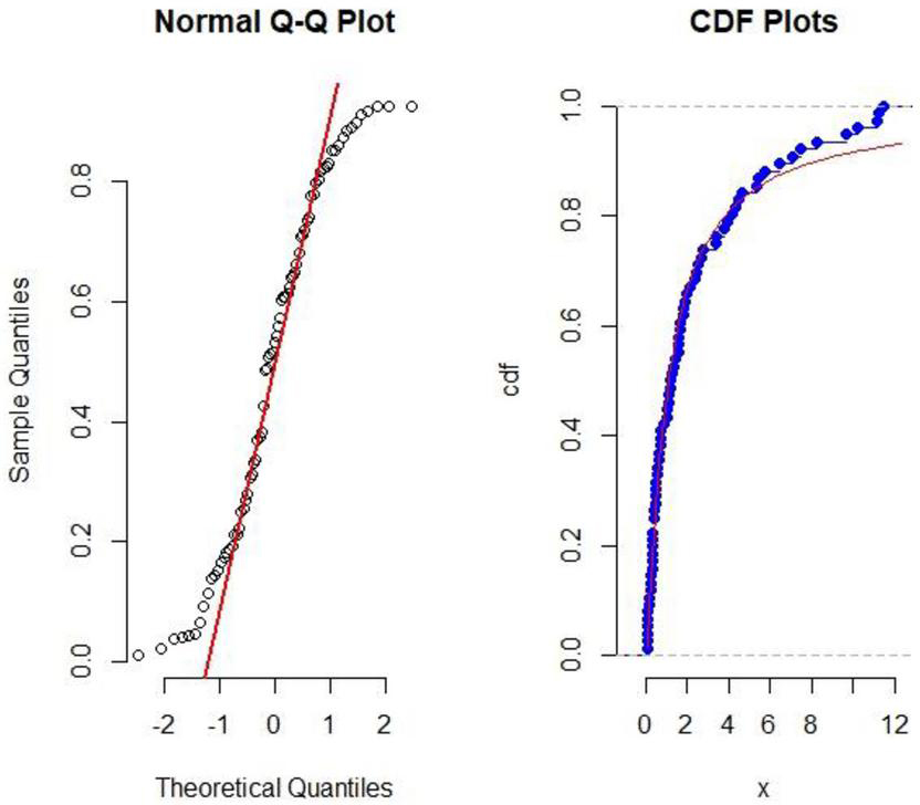
Figure 2 QQ-plot and empirical cdf plot of the IL distribution for COVID-19 mortality data set of United Kingdom of 76 days.

Table 12 MLEs and Bayes estimates of $\alpha$, S(t) and H(t) under APT-II censoring scheme for the COVID-19 mortality data set

							LINEX	GELF
		n	m	CS	MLE	SELF	$-$2	2	$-$2	2
$\alpha$	T $=$ 1.5	76	45	I	1.0546	0.7894	0.7851	0.8279	0.7844	0.7946
				II	1.1581	0.7891	0.7847	0.8276	0.7841	0.7942
				III	1.4721	0.7891	0.7848	0.8276	0.7841	0.7943
	T $=$ 2.5	76	45	I	0.9593	0.6842	0.6797	0.7279	0.6789	0.6902
				II	1.0455	0.6839	0.6794	0.7276	0.6786	0.6899
				III	1.3172	0.6810	0.6769	0.6968	0.6760	0.6854
S(t)	T $=$ 1.5	76	45	I	0.4120	0.3301	0.3307	0.3315	0.3301	0.3315
				II	0.4405	0.3309	0.3305	0.3314	0.3300	0.3314
				III	0.5174	0.3309	0.3305	0.3314	0.3300	0.3314
	T $=$ 2.5	76	45	I	0.3840	0.2941	0.2937	0.2947	0.2930	0.2948
				II	0.4093	0.2940	0.2936	0.2946	0.2929	0.2947
				III	0.4812	0.2931	0.2927	0.2937	0.2920	0.2938
H(t)	T $=$ 1.5	76	45	I	0.5624	0.4210	0.4193	0.4286	0.4184	0.4237
				II	0.6176	0.4208	0.4191	0.4284	0.4182	0.4236
				III	0.7851	0.4208	0.4191	0.4284	0.4182	0.4236
	T $=$ 2.5	76	45	I	0.5116	0.3649	0.3631	0.3732	0.3620	0.3681
				II	0.5576	0.3647	0.3629	0.3731	0.3619	0.3679
				III	0.7025	0.3632	0.3616	0.3667	0.3605	0.3655

For $n=76$, we consider $m=45$ and make same censoring schemes as done in simulation $[I=(0^{14},1^{31})$, $II=(1,0^{14},1^{30})$, $III=(1,2^2,0^{16},1^{26})]$ with both test time $T=1.5$ and $T=2.5$ under APT-II censoring scheme. MLEs and the Bayes estimates are calculated under symmetric and asymmetric loss functions. The calculated estimates of $\alpha$, the survival function $S(t)$ and hazard rate function $H(t)$ as $t=0.75$ with $T=1.5$ and $T=2.5$ are given in Table 12. Table 13 shows the confidence intervals, credible intervals and HPD intervals for the parameter $\alpha$, survival function $S(t)$ and hazard rate function $H(t)$ at $t=0.75$.

Table 13 Classical and Bayesian Interval estimation for $\alpha$, S(t) and H(t) under APT-II censoring scheme for the COVID-19 mortality data set

					Confidence Interval		Credible Interval		HPD interval
		n	m	CS	Interval	AL	Interval	AL	Interval	AL
$\alpha$	T $=$ 1.5	76	45	I	(0.5039,1.6053)	1.1013	(0.7561,0.8129)	0.0568	(0.7561,0.8184)	0.0623
				II	(0.5075,1.8087)	1.3011	(0.7540,0.8209)	0.0669	(0.7499,0.8115)	0.0616
				III	(0.5039,2.4402)	1.9363	(0.7541,0.8200)	0.0659	(0.7528,0.8131)	0.0603
	T $=$ 2.5	76	45	I	(0.4700,1.4485)	0.9784	(0.6563,0.7004)	0.0441	(0.6556,0.6988)	0.0432
				II	(0.4753,1.1404)	1.1404	(0.6560,0.7010)	0.0450	(0.6536,0.6963)	0.0427
				III	(0.4785,2.1558)	1.6773	(0.6532,0.6973)	0.0441	(0.6531,0.6965)	0.0434
S(t)	T $=$ 1.5	76	45	I	(0.4102,0.4139)	0.0037	(0.3279,0.3492)	0.0212	(0.3263,0.3331)	0.0067
				II	(0.4384,0.4426)	0.0041	(0.3277,0.3483)	0.0206	(0.3267,0.3319)	0.0052
				III	(0.5149,0.5199)	0.0049	(0.3279,0.3477)	0.0197	(0.3244,0.3311)	0.0067
	T $=$ 2.5	76	45	I	(0.3824,0.3857)	0.0033	(0.2912,0.3098)	0.0185	(0.2903,0.2944)	0.0041
				II	(0.4075,0.4112)	0.0037	(0.2914,0.3090)	0.0175	(0.2902,0.2933)	0.0031
				III	(0.4789,0.4835)	0.0046	(0.2909,0.3059)	0.0150	(0.2900,0.2933)	0.0032
H(t)	T $=$ 1.5	76	45	I	(0.5587,0.5662)	0.0074	(0.4149,0.4583)	0.0433	(0.4125,0.4231)	0.0105
				II	(0.6131,0.6221)	0.0090	(0.4145,0.4569)	0.0423	(0.4130,0.4212)	0.0081
				III	(0.7778,0.7923)	0.0145	(0.4150,0.4560)	0.0410	(0.4095,0.4199)	0.0104
	T $=$ 2.5	76	45	I	(0.5085,0.5147)	0.0062	(.3594,0.3972)	0.0378	(0.3580,0.3641)	0.0061
				II	(0.5539,0.5613)	0.0074	(0.3597,0.3960)	0.0363	(0.3579,0.3625)	0.0045
				III	(0.6966,0.7083)	0.0116	(0.3590,0.3891)	0.0301	(0.3577,0.3625)	0.0048

8 Conclusion

In this paper, we have considered the classical and Bayesian inference of the unknown shape parameter, survival characteristics (survival and hazard rate function) of the ILD when the data are APT-II censored. The MLEs and the Bayes estimators of the parameter and survival characteristics are obtained. The MLEs are not in closed form. Therefore, numerical approximation technique has been implemented to evaluate them. We have used symmetric (SELF) and symmetric (LINEX, GELF) loss functions to compute the Bayes estimates and their MSEs. Simulation technique MCMC has been done for the different choices of $(n,m)$ combinations to report the performances of the various estimators. Lastly, a COVID-19 mortality data set has been considered to illustrate the computation of various estimators.

References

[1] Adegoke, T. M., Adegoke, G. K., Yahaya, A. M., Uthman, K. T., and Odigie, A. D. (2018). On Bayesian estimation of an exponential distribution. In Proceedings of 2nd International Conference, Professional Statisticians Society of Nigeria (pp. 328–332).

[2] Ahsanullah, M. (1991). Record values of the Lomax distribution. Statistica Neerlandica, 45(1), 21–29.

[3] Aitchison, J., Dunsmore, I.R., (1975). Statistical Prediction Analysis. Cambridge University Press, London.

[4] Albalawi, O., Kabdwal, N. C., Azhad, Q. J., Hora, R., and Alsaedi, B. S. (2022). Estimation of the Generalized Logarithmic Transformation Exponential Distribution under Progressively Type-II Censored Data with Application to the COVID-19 Mortality Rates. Mathematics, 10(7), 1015.

[5] Almetwally, E. M., Almongy, H. M., and ElSherpieny, E. A. (2019). Adaptive type-II progressive censoring schemes based on maximum product spacing with application of generalized Rayleigh distribution. Journal of Data Science, 17(4), 802–831.

[6] Almongy, H. M., Almetwally, E. M., Aljohani, H. M., Alghamdi, A. S., and Hafez, E. H. (2021). A new extended rayleigh distribution with applications of COVID-19 data. Results in Physics, 23, 104012.

[7] Balakrishnan, N., and Ahsanullah, M. (1994). Relations for single and product moments of record values from Lomax distribution. Sankhyā: The Indian Journal of Statistics, Series B, 140–146.

[8] Balakrishnan, N., and Sandhu, R. A. (1995). A simple simulational algorithm for generating progressive Type-II censored samples. The American Statistician, 49(2), 229–230.

[9] Basu, A. P., and Ebrahimi, N. (1991). Bayesian approach to life testing and reliability estimation using asymmetric loss function. Journal of statistical planning and inference, 29(1–2), 21–31.

[10] Berger, J.O., (1980). Statistical Decision Theory Foundations, Concept, and Methods. Springer, New York.

[11] Box GEP and Tiao GC (1973). Bayesian Inference in Statistical Analysis, Addison-Wesley, Mas-sachusetts.

[12] Calabria, R., and Pulcini, G. (1996). Point estimation under asymmetric loss functions for left-truncated exponential samples. Communications in Statistics-Theory and Methods, 25(3), 585–600.

[13] Chaudhary, A. K., and Kumar, V. (2020). A Bayesian Estimation and Predictionof Gompertz Extension Distribution Using the MCMC Method. Nepal Journal of Science and Technology, 19(1), 142–160.

[14] Chen, M. H., and Shao, Q. M. (1999). Monte Carlo estimation of Bayesian credible and HPD intervals. Journal of Computational and Graphical Statistics, 8(1), 69–92.

[15] Cohen, A. C. (1963). Progressively censored samples in life testing. Technometrics, 5(3), 327–339.

[16] Edwards, W., Lindman, H., and Savage, L. J. (1963). Bayesian statistical inference for psychological research. Psychological review, 70(3), 193.

[17] El-Din, M. M., Amein, M. M., El-Attar, H. E., and Hafez, E. H. (2017). Symmetric and Asymmetric Bayesian Estimation For Lindley Distribution Based on Progressive First Failure Censored Data. Math. Sci. Lett, 6(3), 255–260.

[18] El-Din, M. M., Shafay, A. R., and Nagy, M. (2018). Statistical inference under adaptive progressive censoring scheme. Computational Statistics, 33(1), 31–74.

[19] EL-Sagheer, R. M., Mahmoud, M. A., and Nagaty, H. (2019). Statistical inference for Weibull-exponential distribution using adaptive type-II progressive censoring. J Stat Appl Probab, 8(2), 1–13.

[20] Ferguson, T.S., (1967). Mathematical Statistics: A Decision Theoretic Approach. Academic Press, New York.

[21] Goyal, T., Rai, P. K., and Maury, S. K. (2019). Classical and Bayesian studies for a new lifetime model in presence of type-II censoring. Communications for Statistical Applications and Methods, 26(4), 385–410.

[22] Hora, R., Kabdwal, N., Srivastava, P. (2021). Inference for the generalized inverse Lindley distribution under type-II censored data. International journal of statistics and applied mathematics, 6(5), 155–166. doi: 10.22271/maths.2021.v6.i5b.739.

[23] Jan, U., and Ahmad, S. P. (2017). Bayesian analysis of inverse Lomax distribution using approximation techniques. Bayesian Analysis, 7(7), 1–12.

[24] Kleiber, C. (2004). Lorenz ordering of order statistics from log-logistic and related distributions. Journal of Statistical Planning and Inference, 120(1–2), 13–19.

[25] Kleiber, C., and Kotz, S. (2003). Statistical size distributions in economics and actuarial sciences (Vol. 470). John Wiley & Sons.

[26] Kumar, R., Srivastava, A. K., and Kumar, V. (2012). Analysis of Gumbel model for software survival using Bayesian paradigm. International Journal of Advanced Research in Artificial Intelligence, 1(9), 39–45.

[27] Lee, M. Y., and Lim, E. H. (2009). Characterizations of the Lomax, exponential and Pareto distributions by conditional expectations of record values. Journal of the Chungcheong Mathematical Society, 22(2), 149–153.

[28] Lomax, K. S. (1954). Business failures: Another example of the analysis of failure data. Journal of the American Statistical Association, 49(268), 847–852.

[29] Mahmoud, M. A., Soliman, A. A., Abd Ellah, A. H., and El-Sagheer, R. M. (2013). Estimation of generalized Pareto under an adaptive type-II progressive censoring.

[30] Mohan, R., and Chacko, M. (2021). Estimation of parameters of Kumaraswamy-exponential distribution based on adaptive type-II progressive censored schemes. Journal of Statistical Computation and Simulation, 91(1), 81–107.

[31] Mubarak, A.E.S.A.E.G., Almetwally E.M. (2021). A new extension exponential distribution with applications of COVID-19 data. J Fin Business Res. 22:444–60. doi: 10.21608/jsst.2021.51484.1178.

[32] Ng, H. K. T., Kundu, D., and Chan, P. S. (2009). Statistical analysis of exponential lifetimes under an adaptive Type-II progressive censoring scheme. Naval Research Logistics (NRL), 56(8), 687–698.

[33] Rahman, J., Aslam, M., and Ali, S. (2013). Estimation and prediction of inverse Lomax model via Bayesian approach. Caspian Journal of Applied Sciences Research, 2(3), 43–56.

[34] Riad, F. H., and Hafez, E. H. (2020). Point and Interval Estimation for Frechet Distribution Based on Progressive First Failure Censored Data. J. Stat. Appl. Pro, 9, 181–191.

[35] Sewailem, M. F., and Baklizi, A. (2019). Inference for the log-logistic distribution based on an adaptive progressive type-II censoring scheme. Cogent Mathematics & Statistics, 6(1), 1684228.

[36] Shrama, A., and Kumar, P. (2020). Estimation of Parameters of Inverse Lomax Distribution under Type-II Censoring Scheme. Journal of Statistics Applications & Probability, 10(1), 85–102.

[37] Singh, S. K., Singh, U., and Kumar, D. (2013). Bayes estimators of the survival function and parameter of inverted exponential distribution using informative and non-informative priors. Journal of Statistical computation and simulation, 83(12), 2258–2269.

[38] Singh, S. K., Singh, U., and Yadav, A. S. (2016). Survival estimation for inverse Lomax distribution under type $\mathrm{\Pi }$ censored data using Markov chain Monte Carlo method. International Journal of Mathematics and Statistics, 17(1), 128–146.

[39] Sinha, S. K. (1987). Bayesian estimation of the parameters and survival function of a mixture of Weibull life distributions. Journal of statistical planning and inference, 16, 377–387.

[40] Sobhi, M. M. A., and Soliman, A. A. (2016). Estimation for the exponentiated Weibull model with adaptive Type-II progressive censored schemes. Applied Mathematical Modelling, 40(2), 1180–1192.

[41] Soliman, A. A., Abd Ellah, A. H., Abou-Elheggag, N. A., and Modhesh, A. A. (2013). Estimation from Burr type XII distribution using progressive first-failure censored data. Journal of Statistical Computation and Simulation, 83(12), 2270–2290.

[42] Srivastava, A. K. (2020). Estimation of Parameters and Survival Function of Log Gompertz Model: Bayesian Approach under Gamma Prior. International Journal of Advanced Research in Science, Communication and Technology, 10(2), 183–195.

[43] Varian, H.R., (1975). A Bayesian approach to real estate assessment. In: Stephen, E.F., Zellner,A. (Eds.), Studies in Bayesian Econometrics and Statistics in Honor of Leonard J. Savage. North-Holland, Amsterdam, pp. 195–208.

[44] Yadav, A. S., Singh, S. K., and Singh, U. (2016). On hybrid censored inverse Lomax distribution: application to the survival data. Statistica, 76(2), 185–203.

[45] Ye, Z. S., Chan, P. S., Xie, M., and Ng, H. K. T. (2014). Statistical inference for the extreme value distribution under adaptive Type-II progressive censoring schemes. Journal of Statistical Computation and Simulation, 84(5), 1099–1114.

[46] Zellner, A., and Geisel, M. S. (1968). Sensitivity of control to uncertainty and form of the criterion function. In: Donald, G.W. (Ed.), The Future of Statistics. Academic Press, New York, 269–289.

Biographies

Rashi Hora is a research scholar in the department of mathematics and statistics, Banasthali Vidyapith, Rajasthan. Her research area includes survival theory and Bayesian inference. She has the knowledge of many software and languages like R software, OpenBugs and Mathematica.

Naresh Chandra Kabdwal, assistant professor of statistics in the department of mathematics and statistics, Banasthali Vidyapith, Rajasthan. He is having 12 years research experience in various fields of statistics such as sequential analysis, survival theory and Bayesian inference.

Pulkit Srivastava is currently pursuing his Ph.D. at the Department of Statistics, University of Delhi, Delhi. His research areas include Bayesian Inference, Stochastic processes etc.

Journal of Reliability and Statistical Studies, Vol. 15, Issue 2 (2022), 505–534.
doi: 10.13052/jrss0974-8024.1525
© 2022 River Publishers

Abstract

1 Introduction

2 Maximum Likelihood Estimation

3 Bayesian Estimation

3.1 Bayes Estimate Under Symmetric Loss Function

3.2 Bayesian Estimate Under Asymmetric Loss Function

4 Interval Estimation

4.1 Confidence Interval

4.2 Credible Interval and HPD Interval

5 Markov Chain Monte Carlo

6 Simulation Study

7 Real Data Analysis

8 Conclusion

References

Biographies