Analysis of a Stochastic Model with Rework System

Mangey Ram^{1, 2}, Ganga Negi^{3, 4}, Nupur Goyal³ and Anuj Kumar^5,*

¹Department of Mathematics, Computer Science and Engineering, Graphic Era Deemed to be University, Dehradun, India
²Institute of Advanced Manufacturing Technologies, Peter the Great St. Petersburg Polytechnic University, Saint Petersburg, Russia
³Department of Mathematics, Graphic Era Deemed to be University, Dehradun, India
⁴Department of Mathematics, Dev Bhoomi Uttarakhand University, Dehradun, India
⁵Department of Mathematics, University of Petroleum & Energy Studies, Dehradun, India
E-mail: mangeyram@gmail.com; gnegiji@gmail.com; nupurgoyalgeu@gmail.com; anuj4march@gmail.com
*Corresponding Author

Received 14 February 2022; Accepted 07 June 2022; Publication 02 August 2022

Abstract

The demand in the present global industrial system, requires the challenge to meet the growing consumer capabilities and requirements constantly. So, there is always a need to improve different parameters, one of them being different types of failures involved in the working of different engineering systems related to communication systems, manufacturing goods, nuclear and hydro power plants, automobiles and many others. Human error occurring in the working of various systems has always been the challenge to the researchers and is being constantly worked upon by the researchers in the analysis and improvement of reliability and availability of different complex and multistate systems. In the present paper, there is a three-unit system consisting of the unit A with two subunits in parallel and other units B and C are connected in series with A. The authors have investigated and analysed different reliability measures like availability, MTTF and sensitivity taking into account the human failure and carrying out rework system. This research work aims at the study of reliability and availability measures of a multi-state system incorporating human error so as to increase the efficiency of industrial systems by taking maintenance and rework measures to enhance the availability factors. This would help to understand and estimate the reliability measures of any such systems in the field of telecommunication, any electronic devices like that in small power plants, robot systems and such others. Also, a comparison has been made between the availability and reliability estimates in the presence and in the absence of human error. The techniques used are Markov process, Laplace transformation and supplementary variable technique.

Keywords: Multi state model, Markov process, reliability measures and sensitivity analysis.

1 Introduction

For expected effective performance of a system over a period of time, the system needs to be significantly reliable and available. One of the major challenges with researchers is to account for high investments and at the same time justify the time and other resources involved. Different strategies are being employed by the researchers for multi-component systems. Lakhoua (2013) studied with a practical application to a multi-state system like a grain silo. Ram (2013) did a review of the system reliability measures in multi-component systems. Multi-component systems like k-out-of-n: F or k-out-of-n: G systems are like extensions to the present model. Also, for reliability enhancement methods like k-out-of-n systems with active and cold standby systems with redundancy factor are being increasingly developing. Among them are k-out-of-n: F, k-out-of-(n-r): g, k-out-of-(n-r):F, and others. A k-out-of-n: F system proposed by Goyal et al. (2016) evaluated different reliability measures. They also employed the Markov process to carry out the sensitivity analysis of the model. Many other researchers have worked on modified k out of n systems. Likewise, formulation of a reliability function of a shared load system of two-components incorporating perfect coverage was done by Pham (1992) Also, Pham (2010) estimated the reliability of k-out-of-n systems with independent and identical sub units exponentially distributed lifetimes. In these, k-out-of-n systems, tools used for measuring the reliability and other parameters are Markov process, supplementary variable technique and Laplace transformation. Ram and Kumar (2014) presented a 2-out-of-3: F system incorporated with human error. They have evaluated reliability, MTTF and also analysed the sensitivity of the system.

Human error is defined as unsuitable or inappropriate human decisions which can adversely affect the safety, efficiency and overall performance of a system. In the absence of proper identification of the human error in the system the entire system can breakdown completely. Factors responsible for human error are incomplete information regarding the components operation, low quality system design, lack of training of the technicians and helpers hired, inappropriate and insufficient procedure of the entire system, unsuitable tools, uncontrolled level of noise, improper lighting system in the areas of the action. In the state of the error undetected, some of the components may remain in low quality state and make the system risky in terms of safety. So, it is utmost important to construct reliability models with the incorporation of human error to identify the human performance and lead to better guide procedure for the reliability evaluation.

Many researches incorporating human errors (Dhillon (1989), Sawaragi (1999), Sutcliffe and Gregoriades (2007)) have been carried out to identify and improve the reliability of simple and multi-state systems. Dhillon and Yang (1992) stochastically analysed the effect of common cause and human failures on the reliability of a standby system. Dhillon and Yang (1993) also estimated the availability of a man-machine system incorporating critical and non-critical human errors. Dhillon (2014) did an investigative study of human error in maintenance for the factories of the future. Giuntini (2000) proposed a mathematical symbolisation of human reliability for an operation using probabilistic approach to quantify human reliability in a human-machine system. Dhillon and Liu (2006) gave a detailed review of the human errors with the factors responsible and the risks involved and some measures to correct them. El-Damcese and Temraz (2012) estimated various reliability measures and in a parallel system with different failure modes. Gupta and Bansal (1991) estimated the cost of a three-unit stand by system. They analysed the effectiveness of the system at suitable instants. Lin (2010) identified a specified pair of minimal and most reliable paths in a stochastic-flow network (SFN) which can transmit given amount of data under the consideration of constraints of both time and budget. A spare routing is also established to the corresponding reliability. Lastly a convenient method is proposed to establish the best spare path with higher reliability. Ram et al. (2013) presented a stochastic analysis of a two-unit cold standby system incorporating failure due to waiting time to repair. The authors estimated the reliability measures like availability and MTTF of the system with cost analysis. Ram and Singh (2010) analysed a complex system with the incorporation of common cause failure and two types of repair facilities. The authors computed the various transition state probabilities and estimated the expected availability by employing supplementary variable method, Laplace transformation and Gumbel-Hougaard family of copula. Singh et al. (2011) gave an interesting three-component system with one unit controlled by a controller whereas the other two units are independent. The two repairmen employed include the foreman (or the head) and the assistant (or the apprentice). Chaube et al. (2018) applied time-dependent conflicting bi fuzzy set for reliability evaluation. Analysis of a 2-out-of-3: F system with catastrophic failure was done by Tyagi et al. (2019). Supplementary variable technique has been used many researchers in their work. Sirohi et al. (2021) analysed reliability of a complex repairable system in series configuration with a switch under catastrophic failure with copula repair approach. Complex repairable system was stochastically analysed with deliberate failure with emphasis on reboot delay by Kumar and Singh (2016). Singh and Poonia (2022) did the stochastic analysis of k-out-of-n: G type of repairable system in combination of subsystems using controllers and multi repair approach. Poonia (2021) carried out the assessment of performance of multi-state computer network system in series configuration. Performance of a complex repairable system with two subsystems in series configuration with an imperfect switch was analysed by Singh et al. (2020). Kumar et al. (2018a,b, 2019, 2021a,b, 2022), Negi et al. (2021), Uniyal et al. (2022) calculated the availability and cost of various complex systems and optimized the same by using various nature inspired optimization algorithms.

The present paper presents a model with series-parallel combination incorporating human failure. Section 2 comprises of the mathematical model characterisation of the system. It consists of nomenclature associated with the model, transition state diagram with transition states, assumptions and finally shows the formulation of the model along with its solution. Section 3 investigates the particular cases and illustrates the estimation of availability, reliability, MTTF, the expected profit and lastly the analysis of the sensitivity of the model. Section 4 illustrates the conclusions of the proposed inspection.

2 Characteristics of the Mathematical Model

Nomenclature

t	Time-scale.
s	Laplace transformation variable
$S_i$	Transition state for $i=0$, 1, 2, 3, 4, 5, 6, 7
$P_{mnr}^i(t)$	Probability that the system is in $S_i$ state at an epoch “t” for $i=0$ to 7, $m=0,1,2;n=0,1,2;r=0,1,2$
$\overline{P}(s)$	Laplace transformation of $P(t)$
$P_{mnr}^i(x,t)$	Probability density function that the system is in state $S_i$, where i $=$ 2 to 7 at an epoch t and has an elapsed repair time of $x$
${\lambda }_i/{\lambda }_h$	Failure rates for the sub-units. $i=1A,2A,B,C$
$\eta (x)$	Repair rates for the states for $S_i$ where for $i=2$ to 7
$E_p(t)$	Expected profit during the interval [0, $t$)
$K_1,K_2$	Revenue and service cost per unit time, respectively

Table 1 State illustration

State	Illustration
$S_0$	All the units are working in good condition.
$S_1$	The system is in degraded state when sub-unit 2A of A has failed.
$S_2$	The system is in failed state when both sub-unit of A has failed.
$S_3$	The system goes into failed state due to the failure of the sub-unit 2A and then unit B.
$S_4$	The system goes into failed state due to the failure of the sub-unit 2A and then unit C.
$S_5$	The system goes into failed state due to the failure of unit B.
$S_6$	The system goes into failed state due to the failure of unit C.
$S_7$	The system goes into failed state due to human failure.

2.1 System Illustration with Assumptions

In the proposed paper, the system operates in three modes; good state, degraded state and the failed state. All the units and sub-units are identical. The present model consists of three units A, B and C in series. Out of which unit A consists of two sub-units 1A and 2A in parallel. Since the system is a combination of units in series and parallel, the system fails completely in two cases. First, if both the subunits of A fail. Second, if any of the units B or C fails. Also, the system may fail completely in the case of human error. Table 1 notifies the different transition states in the running of the model. Also, the different transition states of the model are described in Figure 1.

The following conditions are assumed for the operation of the model.

(1) Initially, all the components are working in good condition at time $\mathit{\text{t}}=0$.

(2) In the degraded state also, the system is in working state.

(3) All the failure rates and repair rates are constant.

(4) In the situation of the complete failure, the system goes for repair.

(5) The repaired system works as the new one.

(6) The human failure can occur in good or degraded state. In the case of failure due to human-error there is complete breakdown and requires repair.

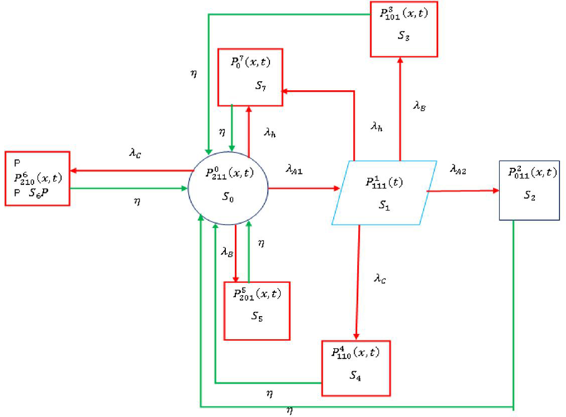
Figure 1 Transition state diagram.

2.2 Conceptualization and Solution of the Mathematical Model

Using Markov process, Laplace transformation and supplementary variable technique following set of differential equation representing the model are obtained –

$$\begin{array}{cc}& \left(\frac{\partial }{\partial t}+\mathrm{\hspace{0.25em}2}{\lambda }_A+{\lambda }_B+{\lambda }_C+{\lambda }_h\right)P_{211}^0(t)\hfill \\ & ={\int }_0^{\mathrm{\infty }}{P}_{011}^2(x,t)\eta (x)\mathrm{\Delta }t\mathit{d}x+{\int }_0^{\mathrm{\infty }}{P}_{101}^3(x,t)\eta (x)\mathrm{\Delta }t\mathit{d}x\hfill \\ & +{\int }_0^{\mathrm{\infty }}{P}_{110}^4(x,t)\eta (x)\mathrm{\Delta }t\mathit{d}x+{\int }_0^{\mathrm{\infty }}{P}_{201}^5(x,t)\eta (x)\mathrm{\Delta }t\mathit{d}x\hfill \\ & +{\int }_0^{\mathrm{\infty }}{P}_{210}^6(x,t)\eta (x)\mathrm{\Delta }t\mathit{d}x+{\int }_0^{\mathrm{\infty }}{P}_c^7(x,t)\eta (x)\mathrm{\Delta }t\mathit{d}x\hfill \end{array}$$	(1)
$$\left(\frac{\partial }{\partial t}+\mathrm{\hspace{0.25em}2}{\lambda }_A+{\lambda }_B+{\lambda }_C+{\lambda }_h\right)P_{111}^1(t)=P_{211}^0(t)2{\lambda }_A$$	(2)
$$\left\{\frac{\partial }{\partial t}+\frac{\partial }{\partial x}+\eta (x)\right\}{P}_{011}^2(t)=0$$	(3)
$$\left\{\frac{\partial }{\partial t}+\frac{\partial }{\partial x}+\eta (x)\right\}{P}_{101}^3(x,t)=0$$	(4)
$$\left\{\frac{\partial }{\partial t}+\frac{\partial }{\partial x}+\eta (x)\right\}{P}_{110}^4(x,t)=0$$	(5)
$$\left\{\frac{\partial }{\partial t}+\frac{\partial }{\partial x}+\eta (x)\right\}{P}_{210}^5(x,t)=0$$	(6)
$$\left\{\frac{\partial }{\partial t}+\frac{\partial }{\partial x}+\eta (x)\right\}{P}_{210}^6(x,t)=0$$	(7)
$$\left\{\frac{\partial }{\partial t}+\frac{\partial }{\partial x}+\eta (x)\right\}{P}_h^7(x,t)=0$$	(8)

Boundary conditions,

$$P_{011}^2(0,t)=P_{111}^1(t){\lambda }_A$$	(9)
$$P_{101}^3(0,t)=P_{111}^1(t){\lambda }_B$$	(10)
$$P_{110}^4(0,t)=P_{111}^1(t){\lambda }_C$$	(11)
$$P_{201}^5(0,t)=P_{211}^0(t){\lambda }_B$$	(12)
$$P_{210}^6(0,t)=P_{211}^0(t){\lambda }_A$$	(13)
$$P_c^7(0,t)=P_{211}^0(t){\lambda }_h+P_{111}^1(t){\lambda }_h$$	(14)

Initial condition

$$P_{211}^0(0)=1$$

(15)

Taking Laplace Transformation of Equations (1) to (14) by the definition: LT of $f(x)=\overline{f(s)}-f(0)$

$$\begin{array}{cc}& (s+2{\lambda }_A+{\lambda }_B+{\lambda }_C+{\lambda }_h)\overline{P_{211}^0}(s)\hfill \\ & =1+{\int }_0^{\mathrm{\infty }}\overline{P_{011}^2}(x,s)\eta (x)\mathit{d}x+{\int }_0^{\mathrm{\infty }}\overline{P_{101}^3}(x,s)\eta (x)\mathit{d}x\hfill \\ & +{\int }_0^{\mathrm{\infty }}\overline{P_{110}^4}(x,s)\eta (x)\mathit{d}x+{\int }_0^{\mathrm{\infty }}\overline{P_{201}^5}(x,s)\eta (x)\mathit{d}x\hfill \\ & +{\int }_0^{\mathrm{\infty }}\overline{P_{210}^6}(x,s)\eta (x)\mathit{d}x+{\int }_0^{\mathrm{\infty }}\overline{P_c^7}(x,s)\eta (x)\mathit{d}x\hfill \end{array}$$	(16)
$$(s+{\lambda }_A+{\lambda }_B+{\lambda }_C+{\lambda }_h)\overline{P_{111}^1}(x,s)=\overline{P_{211}^0}.2{\lambda }_A$$	(17)
$$\left\{s+\frac{\partial }{\partial x}+\eta (x)\right\}\overline{P_{011}^2}(x,s)=0$$	(18)
$$\left\{s+\frac{\partial }{\partial x}+\eta (x)\right\}\overline{P_{101}^3}(x,s)=0$$	(19)
$$\left\{s+\frac{\partial }{\partial x}+\eta (x)\right\}\overline{P_{110}^4}(x,s)=0$$	(20)
$$\left\{s+\frac{\partial }{\partial x}+\eta (x)\right\}\overline{P_{201}^5}(x,s)=0$$	(21)
$$\left\{s+\frac{\partial }{\partial x}+\eta (x)\right\}\overline{P_{210}^6}(x,s)=0$$	(22)
$$\left\{s+\frac{\partial }{\partial x}+\eta (x)\right\}\overline{P_c^7}(x,s)=0$$	(23)
$$\overline{P_{011}^2}(0,s)=\overline{P_{111}^1}(s).{\lambda }_A$$	(24)
$$\overline{P_{101}^3}(0,s)=\overline{P_{111}^1}(s).{\lambda }_B$$	(25)
$$\overline{P_{110}^4}(0,s)=\overline{P_{111}^1}(s).{\lambda }_C$$	(26)
$$\overline{P_{101}^5}(0,s)=\overline{P_{211}^0}(s).{\lambda }_B$$	(27)
$$\overline{P_{210}^6}(0,s)=\overline{P_{211}^0}(s).{\lambda }_C$$	(28)
$$\overline{P_C^7}(0,s)=\overline{P_{211}^0}(s).+\overline{P_{111}^1}(s).{\lambda }_h$$	(29)

After solving Equations (16) to (23) using Equations (24) to (29), we get

$\overline{P_{211}^0}(s)$	$={\displaystyle \frac{1}{[s+c_1-\overline{\underset{\mathrm{\infty }}{\underbrace{S(s)}}}\{({\lambda }_B+{\lambda }_C+{\lambda }_h)+\frac{\overline{c_2}2{\lambda }_A}{s+c_2}]}}$	(30)
$\overline{P_{111}^1}(s)$	$={\displaystyle \frac{2{\lambda }_A\overline{P_{211}^0}(s)}{s+c_2}}$	(31)
$\overline{P_{011}^2}(s)$	$={\displaystyle \frac{2{\lambda }_A{\lambda }_A(1-\overline{\underset{\mathrm{\infty }}{\underbrace{S(s)}}})}{s(s+c_{2)}}}\overline{P_{211}^0}(s)$	(32)
$\overline{P_{101}^3}(s)$	$={\displaystyle \frac{2{\lambda }_A{\lambda }_B(1-\overline{\underset{\mathrm{\infty }}{\underbrace{S(s)}}})}{s(s+c_{2)}}}\overline{P_{211}^0}(s)$	(33)
$\overline{P_{011}^4}(s)$	$={\displaystyle \frac{2{\lambda }_A{\lambda }_C(1-\overline{\underset{\mathrm{\infty }}{\underbrace{S(s)}}})}{s(s+c_{2)}}}\overline{P_{211}^0}(s)$	(34)
$\overline{P_{201}^5}(s)$	$={\displaystyle \frac{{\lambda }_B(1-\overline{\underset{\mathrm{\infty }}{\underbrace{S(s)}}})}{s(s+c_{2)}}}\overline{P_{211}^0}(s)$	(35)
$\overline{P_{210}^6}(s)$	$={\displaystyle \frac{2{\lambda }_A{\lambda }_C(1-\overline{\underset{\mathrm{\infty }}{\underbrace{S(s)}}})}{s(s+c_{2)}}}\overline{P_{211}^0}(s)$	(36)
$\overline{P_C^7}(s)$	$={\displaystyle \frac{[s+c_2+2{\lambda }_A](1-\overline{\underset{\mathrm{\infty }}{\underbrace{S(s)}}})}{s(s+c_{2)}}}\overline{P_{211}^0}(s)$	(37)

where,

$$2{\lambda }_A+{\lambda }_B+{\lambda }_C+{\lambda }_h=c_1;{\lambda }_A+{\lambda }_B+{\lambda }_C+{\lambda }_h=c_2$$

and

$${\int }_0^{\mathrm{\infty }}\exp [-sx-{\int }_0^x\eta (x)]\eta (x)dx]dx=\overline{\underset{\mathrm{\infty }}{\underbrace{S(s)}}}$$

System Uptime Probability

$\overline{{\mathrm{P}}_{\mathrm{up}}}(\mathrm{s})$	$=\overline{P_{211}^0}(s)+\overline{P_{111}^1}(s)$
$\overline{{\mathrm{P}}_{\mathrm{up}}}(\mathrm{s})$	$={\displaystyle \frac{1}{[s+c_1-\overline{\underset{\mathrm{\infty }}{\underbrace{S(s)}}}\{({\lambda }_B+{\lambda }_C+{\lambda }_h)+\frac{\overline{c_2}2{\lambda }_A}{s+c_2}]}}\left[1+{\displaystyle \frac{2{\lambda }_A}{s+c_2}}\right]$

System Downtime Probability

$$\overline{{\mathrm{P}}_{\mathrm{down}}}(\mathrm{s})=\overline{P_{011}^2}(s)+\overline{P_{101}^3}+\overline{m}(s)+\overline{P_{201}^5}(s)+\overline{P_{210}^6}(s)+\overline{P_C^7}(s)$$

Using Equations (32) to (37)

$$\overline{{\mathrm{P}}_{\mathrm{down}}}(\mathrm{s})=\overline{P_{211}^0}(s)\frac{(1-\overline{\underset{\mathrm{\infty }}{\underbrace{S(s)}}})}{s}\left[\frac{2{\lambda }_A{c}_2}{(s+c_{2)}}+{\lambda }_B+{\lambda }_C+{\lambda }_h\right]$$

(39)

Now, solving Equations (38) and (39), we obtain

$$\overline{{\mathrm{P}}_{\mathrm{up}}}(\mathrm{s})+\overline{{\mathrm{P}}_{\mathrm{down}}}(s)=\frac{1}{s}$$

(40)

3 Particular Cases

3.1 Availability Analysis

In general, availability is a measure of the performance of maintained equipment. The steady-state availability is defined as the proportion of time during which a system is available for use. In the given model, putting the different values of failure rates as ${\lambda }_A=0.02$, ${\lambda }_B=0.05$, ${\lambda }_C=0.03$, ${\lambda }_h=0.02$ and the repair rates as $\eta =1$ in the Equation (38) followed by taking the inverse Laplace transform, the availability of the model is obtained as follows –

$P_{up}(t)$	$=0.09252208159e^{(-1.103287720t)}$
	$\mathrm{\hspace{1em}}+0.9074779182e^{(-0.07835613991t)}\cos (0.05061206776t)$
	$\mathrm{\hspace{1em}}+1.445997890e^{(-0.07835613991t)}\sin (0.05061206776t)$	(41)

Now changing the time starting from $\mathit{\text{t}}=0$ to $\mathit{\text{t}}=10$ in Equation (41), and get the different values of availability as given in Table 2 and Figure 2.

Table 2 Availability as function of time

Time	Availability $P_{up}(t)$
0	1.0000
1	0.9363
2	0.9070
3	0.8854
4	0.8634
5	0.8388
6	0.8115
7	0.7817
8	0.7499
9	0.7168
10	0.6827

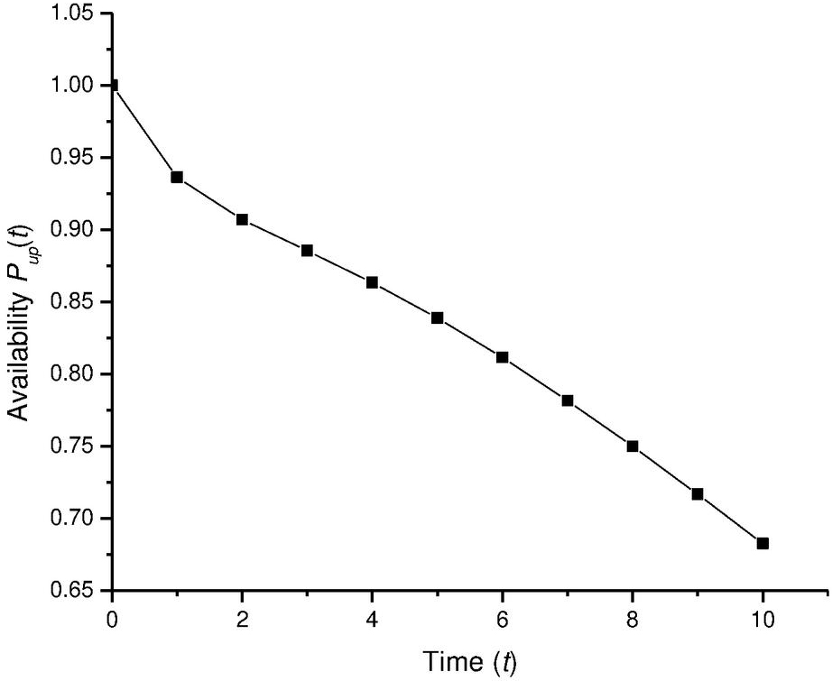
Figure 2 Variations of availability with time.

3.2 Availability in the Absence of Human Error

In the situation of absence of human error, the failure due to human error is zero. So, we put ${\lambda }_h=0$ and other failure rates as ${\lambda }_A=0.02$, ${\lambda }_B=0.05$, ${\lambda }_C=0.03$, ${\lambda }_h=0.02$ along with the repair rate as $\eta =1$ in the Equation (38) followed by the inverse Laplace transformation to get the availability of the model is obtained as follows –

$P^{\prime }(t)$	$=0.09252208159e^{(-1.103287720t)}$
	$\mathrm{\hspace{1em}}+0.9074779182e^{(-0.07835613991t)}\cos (0.05061206776t)$
	$\mathrm{\hspace{1em}}+1.445997890{\mathrm{e}}^{(-0.07835613991\mathrm{t})}\sin (0.05061206776\mathrm{t})$	(42)

Increasing the time from $\mathit{\text{t}}=0$ to $\mathit{\text{t}}=10$ in Equation (42) the variations in availability obtained are shown in the Table 3 and Figure 3

Table 3 Availability as function of time

Time	Availability $P^{\prime }(t)$
0	0.999999998
1	0.9363
2	0.9070
3	0.8854
4	0.8634
5	0.8388
6	0.8115
7	0.7817
8	0.7499
9	0.7168
10	0.6827

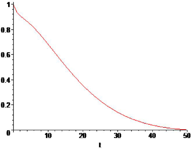
Figure 3 Variations of availability with time.

3.3 Reliability

While the status of the equipment defines its availability, failure-free operation up to a certain time emphasises on its reliability. For reliability, $\eta =0$. In the present model, reliability can be calculated by taking the values of failure rates as ${\lambda }_A=0.02$, ${\lambda }_B=0.05$, ${\lambda }_C=0.03$, ${\lambda }_h=0.02$ and repair rate $\eta =0$ in Equation (38) followed by inverse Laplace transform we get the reliability of the system as

$$R(t)=0.4375949e^{(0.13t)}sin(0.068556546t)+e^{(0.13t)}cos(0.068556546t)$$

(43)

Table 4 Variation of reliability with time

Time	Reliability $R(t)$
0	1.0000
1	0.9023
2	0.8099
3	0.7233
4	0.6427
5	0.5684
6	0.5004
7	0.4384
8	0.3822
9	0.3317
10	0.2865

On changing the time from $\mathit{\text{t}}=0$ to $\mathit{\text{t}}=10$ in Equation (43), we obtain the different values of reliability as shown in Table 4 and Figure 4.

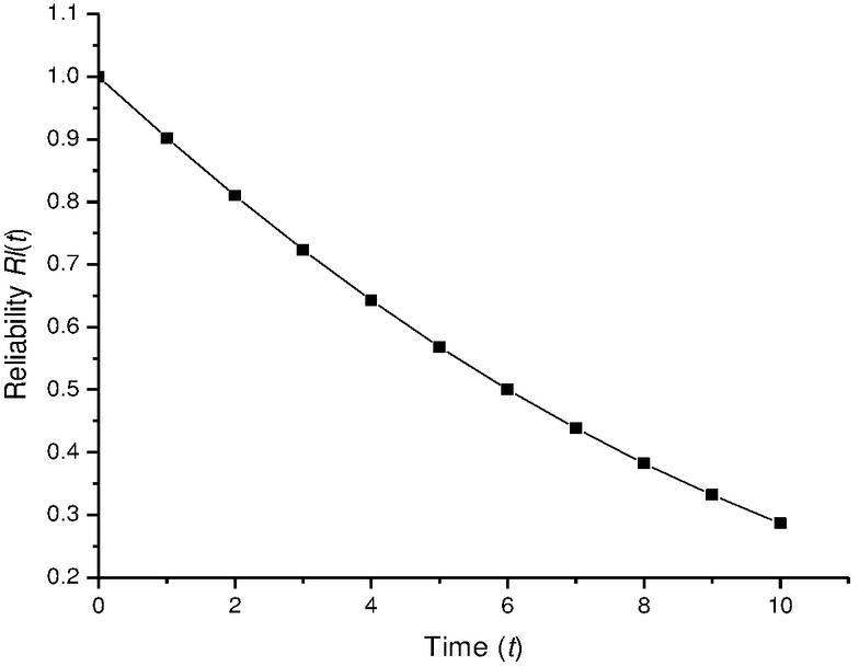
Figure 4 Variation of reliability with time.

3.4 Reliability in the Absence of Human Error

In the case of human error being zero ${\lambda }_h=0$. To estimate reliability in the absence of human error, we take values of failure rates as ${\lambda }_A=0.02$, ${\lambda }_B=0.05$, ${\lambda }_C=0.03$, and repair rates $\eta =0$ in Equation (38) followed by the inverse Laplace transform. The resulting expression for reliability is given below.

$R^{\prime }(t)$	$=0.4803844614e^{(-0.1100000000t)}\sin (0.06244997998t)$
	$\mathrm{\hspace{1em}}+e^{(-0.1100000000t)}\cos (0.06244997998t)$	(44)

Table 5 Variation of reliability with time

Time	Reliability $R^{\prime }(t)$
0	1.0000
1	0.9209
2	0.8442
3	0.7706
4	0.7005
5	0.6341
6	0.5718
7	0.5136
8	0.4595
9	0.4095
10	0.3635
40	$-$0.0062

The corresponding variations in values of the reliability of the system with the increase in time from $\mathit{\text{t}}=0$ to $\mathit{\text{t}}=10$ and $\mathit{\text{t}}=40$ are obtained from Equation (44) and shown in the Table 5 and Figure 5.

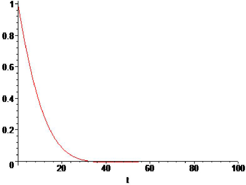
Figure 5 Variation of reliability with time.

3.5 MTTF

MTTF means the average of the sum duration of the total time to failure of a system completely. For MTTF analysis of the present model, substitute the same failure rates as ${\lambda }_A=0.02$, ${\lambda }_B=0.05$, ${\lambda }_C=0.03$, ${\lambda }_h=0.02$ and repair rate $\eta =0$ in Equation (38), along with $s$ tending to zero. The expression for MTTF so obtained is as shown below.

$$M=\frac{1}{2({\lambda }_A+{\lambda }_B+{\lambda }_C+{\lambda }_h)}+\frac{1}{4{\lambda }_A}$$

(45)

To find the variation in the MTTF, taking the failure rates as mentioned above along with the variation in the failure rates from 0.1 to 0.9 one after the other in Equation (45). The corresponding values of MTTF obtained are given below in the Table 6 and also presented by Figure 6.

Table 6 MTTF as function of time

Change in	Changes in MTTF with Change in Failure Rates
Failure Rates	${\lambda }_A$	${\lambda }_B$	${\lambda }_C$	${\lambda }_h$
0.01	29.5454	18.7500	17.5000	17.0454
0.02	16.6667	18.0556	17.0454	16.6667
0.03	12.1795	17.5000	16.6667	16.3461
0.04	9.8214	17.0454	16.3461	16.0714
0.05	8.3334	16.6667	16.0714	15.8333
0.06	7.2917	16.3461	15.8333	15.6250
0.07	6.5126	16.0714	15.6250	15.4412
0.08	5.9028	15.8333	15.4412	15.2778
0.09	5.4093	15.6250	15.2778	15.1316

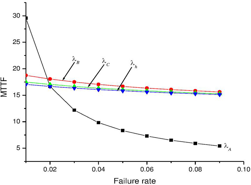
Figure 6 MTTF as function of time.

It is clear that with the increase in the values of the failure rate, the values of MTTF shows decrease gradually for units B and C while for A it reduces drastically and becomes the least. Figure 4 shows a curvilinear behaviour of the MTTF for unit A.

3.6 Expected Profit

A system requires service cost for the service facility provided [23, 24] and to calculate the expected profit during the time interval [0, t),the following equation is used.

$$E_{up}(t)=K_1{\int }_0^t{P}_{up}(t)\mathit{d}t-K_{2}t.$$

(46)

Here $K_1$ is the revenue cost and $K_2$ is the service cost. For fixed value of $K_1$ and varying the values of $K_2$ from 0.1 to 0.5 the values of expected profit are computed using Equation (38) in Equation (46) as given in Table 7 and the graphical representation in Figure 7.

Table 7 Variation of Expected profit with time

Time (t)	${\mathrm{K}}_2=0.1$	${\mathrm{K}}_2=0.2$	${\mathrm{K}}_2=0.3$	${\mathrm{K}}_2=0.4$	${\mathrm{K}}_2=0.5$
0	0.0000	0.0000	0.0000	0.0000	0.0000
1	0.8632	0.7632	0.6632	0.5632	0.4632
2	1.6836	1.4836	1.2836	1.0836	0.8836
3	2.4796	2.1796	1.8796	1.5796	1.2796
4	3.2542	2.8542	2.4542	2.0542	1.6542
5	4.0055	3.5055	3.0055	2.5055	2.0055
6	4.7309	4.1309	3.5309	2.9309	2.3309
7	5.4277	4.7277	4.0277	3.3277	2.6277
8	6.0937	5.2937	4.4937	3.6937	2.8937
9	6.7272	5.8272	4.9272	4.0272	3.1272
10	7.3270	6.3270	5.3270	4.3270	3.3270

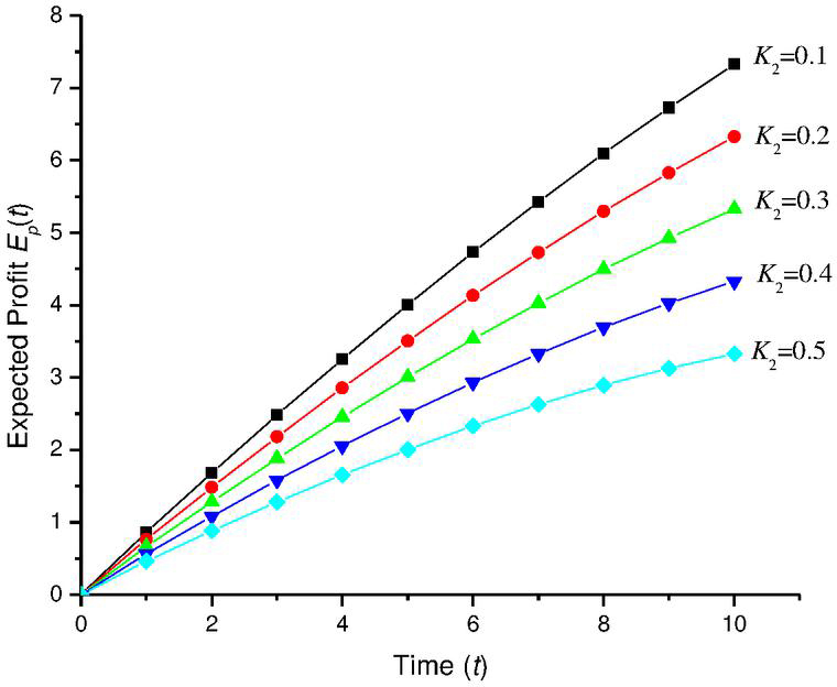
Figure 7 Variation of expected profit with time.

It is clearly illustrated from Figure 7 that as the time increases, with fixed revenue cost $K_1=1$ and changing the service cost $K_2=0.1,0.2$ up to $0.5$, gradually increases the expected profit. The service cost is varied to account for the maintenance conditions.

3.7 Sensitivity Analysis

Sensitivity is a parameter which checks the efficiency of the system to the fullest. The sensitivity analysis helps the researchers to work upon the reliability measures and quality enhancement technologies.

3.7.1 Sensitivity of availability

For the sensitivity of availability of the system, putting $\eta =1$ in Equation (38). Then the values of the partial derivatives $\frac{\partial P_{up}(t)}{\partial {\lambda }_A}$, $\frac{\partial P_{up}(t)}{\partial {\lambda }_{B,}}$, $\frac{\partial P_{up}(t)}{\partial {\lambda }_C}$ and $\frac{\partial P_{up}(t)}{\partial {\lambda }_h}$ are obtained by taking failure rates as ${\lambda }_A=0.02$, ${\lambda }_B=0.05$, ${\lambda }_C=0.03$, ${\lambda }_h=0.02$ and varying time from $\mathit{\text{t}}=0$ to $\mathit{\text{t}}=10$ to obtain the sensitivity of availability of the components as shown in Table 8 and illustrated by the Figure 8.

Table 8 Sensitivity of availability as function of time

Time (t)	${\displaystyle \frac{\partial P_{up}(t)}{\partial {\lambda }_A}}$	${\displaystyle \frac{\partial P_{up}(t)}{\partial {\lambda }_B}}$	${\displaystyle \frac{\partial P_{up}(t)}{\partial {\lambda }_C}}$	${\displaystyle \frac{\partial P_{up}(t)}{\partial {\lambda }_h}}$
0	0.0000	0.0000	0.0000	0.0000
1	-0.1832	-0.6019	-0.6019	-0.6019
2	-0.7168	-0.8326	-0.8326	-0.8326
3	-1.5471	-0.9680	-0.9680	-0.9680
4	-2.6094	-1.0841	-1.0841	-1.0841
5	-3.8421	-1.1979	-1.1979	-1.1979
6	-5.1903	-1.3100	-1.3100	-1.3100
7	-6.6060	-1.4174	-1.4174	-1.4174
8	-8.0483	-1.5164	-1.5164	-1.5164
9	-9.4824	-1.6042	-1.6042	-1.6042
10	-10.8794	-1.6787	-1.6787	-1.6787

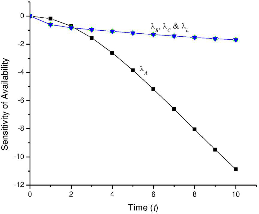
Figure 8 Sensitivity of availability as function of time.

It can be clearly seen that as the time increases, the component A becomes least sensitive to availability as compared to other. Also, Table 8 clearly signifies that with regard to the failure of the sub-system B and C and also with regard to human failure, the sensitivity of the system is unexpectedly exactly equal. Figure 8 shows a sharp decline in the curve for unit A.

3.7.2 Sensitivity of reliability

A system also becomes sensitive to reliability as time passes. For computing sensitivity of reliability of the system, put $\eta =0$ in Equation (38). On differentiating the resulting expression with respect to different failure rates ${\lambda }_A$, ${\lambda }_B$, ${\lambda }_C$ and ${\lambda }_h$ and then the values of the partial derivatives, $\frac{\partial R(t)}{\partial {\lambda }_A}$, $\frac{\partial R(t)}{\partial {\lambda }_B}$, $\frac{\partial R(t)}{\partial {\lambda }_C}$, and $\frac{\partial R(t)}{\partial {\lambda }_h}$ are obtained by taking failure rates as ${\lambda }_A=0.02$, ${\lambda }_B=0.05$, ${\lambda }_C=0.03$, ${\lambda }_h=0.02$ and varying time from $\mathit{\text{t}}=0$ to $\mathit{\text{t}}=10$ as shown in Table 9 and Figure 9.

Table 9 Sensitivity of reliability as function of time

Time (t)	${\displaystyle \frac{\partial R(t)}{\partial {\lambda }_A}}$	${\displaystyle \frac{\partial R(t)}{\partial {\lambda }_B}}$	${\displaystyle \frac{\partial R(t)}{\partial {\lambda }_C}}$	${\displaystyle \frac{\partial R(t)}{\partial {\lambda }_h}}$
0	28.4362	4.2128	4.2128	4.2128
1	25.5025	2.8813	2.8813	2.8813
2	22.4841	1.7295	1.7295	1.7295
3	19.4968	0.7525	0.7525	0.7525
4	16.6245	-0.0587	-0.0587	-0.0587
5	13.9258	-0.7163	-0.7163	-0.7163
6	11.4387	-1.2346	-1.2346	-1.2346
7	9.1852	-1.6283	-1.6283	-1.6283
8	7.1747	-1.9129	-1.9129	-1.9129
9	5.4072	-2.1031	-2.1031	-2.1031
10	3.8755	-2.2131	-2.2131	-2.2131

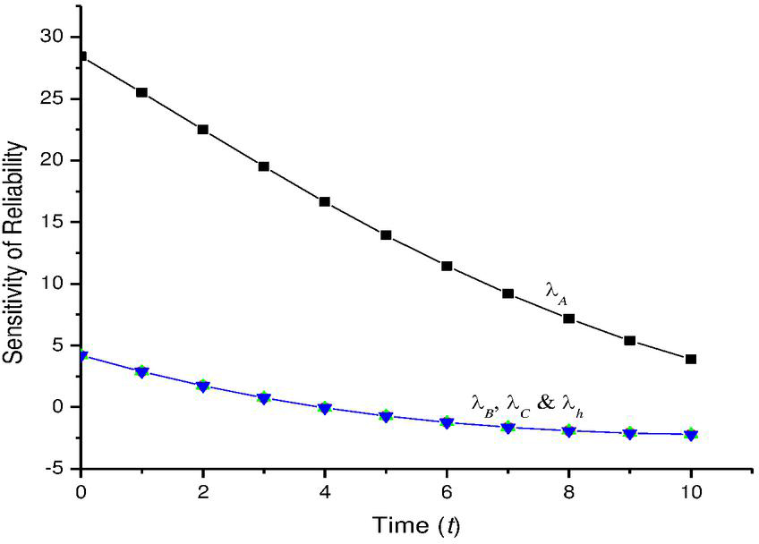
Figure 9 Sensitivity of reliability as function of time.

Figure 9 is very illustrative. In the beginning the gap of sensitivity of the unit A and that of units B and C together is much higher but decreases gradually. Unit A remains most sensitive to reliability as compared to other units as well as the human error, though decreases sharply with time.

3.7.3 Sensitivity of MTTF

In general, the sensitivity of the MTTF of the system increases with the increase in the failure rates. Sensitivity of MTTF can be studied by differentiating Equation (45) with respect to different failure rates to obtain the partial derivatives $\frac{\partial M}{\partial {\lambda }_A}$, $\frac{\partial M}{\partial {\lambda }_B}$, $\frac{\partial M}{\partial {\lambda }_C}$ and $\frac{\partial M}{\partial {\lambda }_h}$ and then obtaining their values for different failure rates ${\lambda }_A=0.02$, ${\lambda }_B=0.05$, ${\lambda }_C=0.03$, ${\lambda }_h=0.02$. Table 10 and Figure 10 illustrate the sensitivity of MTTF of the system with the passage of time.

Table 10 Sensitivity of reliability as function of time

Change in Failure Rates	${\displaystyle \frac{\partial M}{\partial {\lambda }_A}}$	${\displaystyle \frac{\partial M}{\partial {\lambda }_B}}$	${\displaystyle \frac{\partial M}{\partial {\lambda }_C}}$	${\displaystyle \frac{\partial M}{\partial {\lambda }_h}}$
0.01	-2541.3223	-78.1250	-50.0000	-41.3223
0.02	-659.7222	-61.7284	-41.3223	-34.7222
0.03	-307.3636	-50.0000	-34.7222	-29.5858
0.04	-181.7602	-41.3223	-29.5858	-25.5102
0.05	-122.2222	-34.7222	-25.5102	-22.2222
0.06	-88.9757	-29.5858	-22.2222	-19.5312
0.07	-68.3214	-25.5102	-19.5312	-17.3010
0.08	-54.4946	-22.2222	-17.3010	-15.4321
0.09	-44.7146	-19.5312	-15.4321	-13.8504

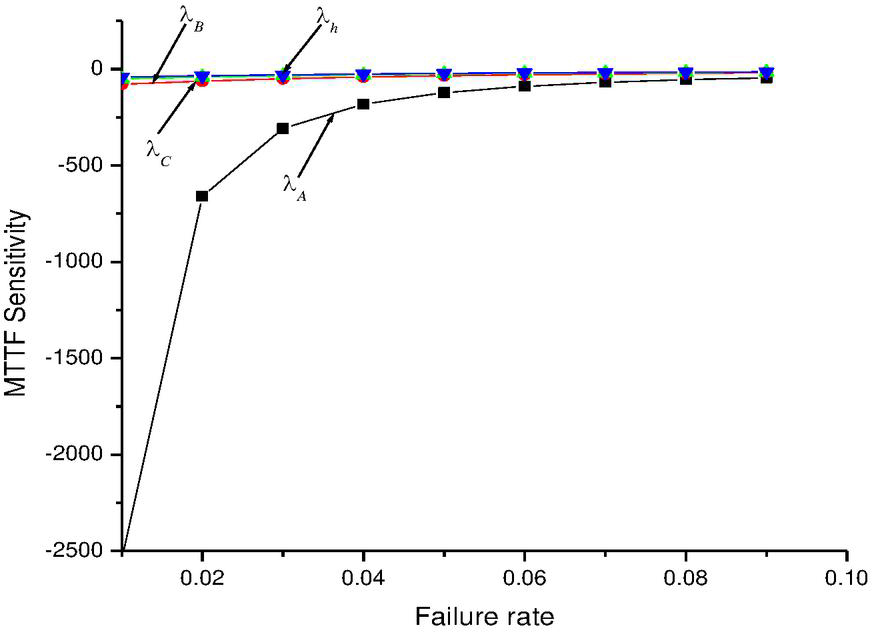
Figure 10 Sensitivity of MTTF as function of time.

4 Conclusion & Future Scope

The proposed system presents the behaviour of a system under the influence of human error together with the unit failure with the increase in time. Also, it presents a detailed variation in the different reliability measures like reliability, availability, MTTF and system sensitivity to these reliability measures with variation in the failure rates of the units as well as human failure. The obtained results are as follows –

(i) A decrease in the availability, reliability as well as MTTF of the system is witnessed with the passage of time as shown in Tables 2, 4 and 6 as well as Figures 2, 4 and 6. In fact, reliability becomes lower than availability.

(ii) In the absence of human error the availability is exactly the same as in the presence of human error because there is simultaneous repair facility available for the rework system as given in the Tables 2, 3 and Figures 4, 5. On the contrary a comparison of the reliability values in the presence and in the absence of human shows that reliability values are higher in the absence of human error and also the decrease in the reliability is slower as can be seen in the Table 5 and Figure 5.

(iii) MTTF is highest in the beginning and becomes the least gradually with the passage of time for the unit A. The Figure 6 and Table 6 clearly high light the variations in the values of MTTF. The behaviour of the MTTF of unit A is slightly different than the others. Also, for some values of failure rate the MTTF values of the two units B and C are same.

(iv) Expected profit of the system shows increment as illustrated in Table 7 and Figure 7 though for the maintenance of the system, service cost increases.

(v) Sensitivity analysis of the system as shown in Tables 8, 9 and 10 shows that unit A is least sensitive to availability and reliability as compared to units B and C or even to human failure. Figures 8, 9 and 10 illustrate this fact more visibly. In fact, sensitivity of availability with respect to unit A decreases sharply.

(vi) With respect to unit A sensitivity of MTTF is the least whereas it is the highest with respect to human failure as depicted in Table 10 and Figure 10. Also, with respect to unit A it increases sharply as compared to that of B and C as also that of human failure sensitivity.

Sensitivity being a very delicate issue for any system so, the scope of such a system in future lies in the fact that the researches can be done to control the sensitivity to increase the reliability and hence the profit. This proposed model can be a starting point and can be extended to systems with increased number of units incorporating more types of failures to develop some systems with the better achievable reliability measures and higher expected profit. This can be used to develop more reliable and cost-efficient systems. Also, it can be extended to k-out-of-n systems. Further quantification of human reliability using probabilistic approach can be a field of research particularly with complex multistate systems so as to estimate reliability measures more efficiently.

References

Chaube, S., Singh, S.B., Pant, S., Kumar, A. (2018): Time-dependent conflicting bi fuzzy set and its app lications in reliability evaluation, Advanced Mathematical Techniques in Engineering Sciences, 111–128.

Dhillon, B. S. (2014): Human error in maintenance: An investigative study for the factories of the future. IOP Conference Series: Materials Science and Engineering, Volume 65, 27th International Conference on CADCAM, Robotics and Factories of the Future 2014 22–24 July 2014, London, UK

Dhillon, B. S., Yang, N.(1992): Stochastic analysis of standby systems with common cause failures and human errors. Micro-electron Reliability 32(12), 1699–1712 (1992).

Dhillon, B. S., Yang, N.(1993): Availability of a man-machine system with critical and non-critical human errors. Micro-electron Reliability 33(10), 1511–1521 (1993).

Dhillon, B.S., and Liu, Y. (2006): Human errors in maintenance: a review. J. Qual. Maint. Eng. 12(1), 21–36.

Dhillon, B.S.: (1989):Human errors: a review. Microelectron. Reliab. 29(3), 299-304. Ram, M., and Kumar A (2014): Performance of a structure consisting of a 2-out-of-3: F substructure under human failure. Arabian Journal for Science and Engineering, 39(11), 8383–8394.

Dhillon, B.S.: (1989):Human errors: a review. Microelectron. Reliab. 29(3), 299–304.

El-Damcese, M.A., and Temraz, N. S. (2012): Analysis for a parallel repairable system with different failure modes. Journal of Reliability and Statistical Studies, 5(1), 95-106.

Giuntini, R.E. (2000): Mathematical characterization of human reliability for multi-task system operations. IEEE International Conference on Systems, Man, and Cybernetics, 2, 1325–1329.

Goyal, N., Ram, M., Amoli, S., and Suyal, A. (2016): Sensitivity analysis of a three-unit series system under k-out-of-n redundancy. International Journal of quality and reliability maintenance, 34, 770–784.

Gupta, R., and Bansal, S. (1991): Cost analysis of a three-unit standby system subject to random shocks and linearly increasing failure rates. Reliability Engineering and System Safety, 33, 249–263.

Kumar, A., Negi, G., Pant, S., Ram, M. (2021b): Availability-Cost Optimization of Butter Oil Processing System by Using Nature Inspired Optimization Algorithms. Reliability: Theory & Applications, SI 2(64), 188–200.

Kumar, A., Pant, S., & Ram, M. (2019): Gray wolf optimizer approach to the reliability-cost optimization of residual heat removal system of a nuclear power plant safety system. Quality and Reliability Engineering International, 35(7), 2228–2239.

Kumar, A., Pant, S., Ram, M. (2018a): Complex System Reliability Analysis and Optimization, Advanced Mathematical Techniques in Science and Engineering, 1, River Publishers, 185–199.

Kumar, A., Pant, S., Ram, M., & Yadav, O. (Eds.). (2022). Meta-heuristic Optimization Techniques: Applications in Engineering (Vol. 10). Walter de Gruyter GmbH & Co KG.

Kumar, A., Ram, M., Pant, S. and Kumar, A. (2018b): Industrial System Performance under Multistate Failures with Standby Mode. Modeling and Simulation in Industrial Engineering, 85–100.

Kumar, A., Vohra, M., Pant, S., & Singh, S. K. (2021a). Optimization techniques for petroleum engineering: A brief review. International Journal of Modelling and Simulation, 41(5), 326–334.

Kumar, D. and Singh, S.B. (2016) ‘Stochastic analysis of the complex repairable system with deliberate failure emphasizing reboot delay’, Communication in Statistics – Simulation and Computation, Vol. 45, No. 2, pp. 1–20.

Lakhoua, M.N. (2013): Systemic analysis of an industrial system: case study of a grain silo. Arabian, J. Sci. Eng. 38(5), 1243–1254.

Lin, Yi-K. (2010):Spare Routing Reliability for a Stochastic Flow Network Through Two Minimal Paths Under Budget constraint. IEEE transactions on reliability, 59(1), 2–10.

Negi, G., Kumar, A., Pant, S., and Ram, M. (2021): GWO: a review and applications. International Journal of System Assurance Engineering and Management, 12(1), 1–8.

Pham, H. (1992): Reliability analysis of a high voltage system with dependent failures and imperfect coverage. Reliability Engineering and System Safety, 37(1), 25–28.

Pham, H. (2010): On the estimation of reliability of k-out-of-n systems. Int. J. Syst. Assur. Eng. Manag. 1(1), 32–35.

Poonia, P.K. (2021) Performance assessment of a multi-state computer network system in series configuration using copula repair. Int. J. Reliability and Safety, Vol. 15, No. 1/2, pp. 68–88.

Ram, M. (2013): On system reliability approaches: a brief survey. Int. J. Syst. Assur. Eng. Manag. 4(2), 101–117.

Ram, M., and Kumar A (2014): Performance of a structure consisting of a 2-out-of-3: F substructure under human failure. Arabian Journal for Science and Engineering, 39(11), 8383–8394.

Ram, M., and Singh, S. B. (2010): Analysis of a complex system with common cause failure and two types of repair facilities with different distributions in failure. Int J Reliab, 4(4), 381–392.

Ram, M., Singh, S. B., and Singh, V.V. (2013): Stochastic Analysis of a Standby System with Waiting Repair Strategy. IEEE Transactions on Systems, Man and Cybernetics, 43(3), 698–707.

Sawaragi, T. (1999): Modelling and analysis of human interactions with and within complex systems. IEEE International Conference on Systems, Man, and Cybernetics, 1, 701–707.

Singh, S. B., Ram M., and Chaube, S. (2011): Analysis of the reliability of a three-component system with two repairmen. IJE Trans. A, Basics, 24(4), 395–402.

Singh, V.V. and Poonia, P. K. (2022) Stochastic analysis of k-out-of-n: G type of repairable system in combination of subsystems with controllers and multi repair approach. Journal of Optimization in Industrial Engineering, Vol. 15, No. 1, pp. 121–130.

Singh, V.V., Poonia, P.K. and Adbullahi, A.H. (2020). Performance analysis of a complex repairable system with two subsystems in series configuration with an imperfect switch, J. Math. Comput. Sci., 10(2), pp. 359–383.

Sirohi, A., Poonia, P. K. and Raghav, D. (2021):Reliability analysis of a complex repairable system in series configuration with switch and catastrophic failure using copula repair, J. Math. Comput. Sci., 11 (2), pp. 2403-2425.

Sutcliffe, A.G., and Gregoriades, A. (2007): Automating scenario analysis of human and system reliability. IEEE Trans. Syst. Man Cybern. Part A Syst. Hum. 37(2), 249–261.

Tyagi, V., Arora, R., Ram, M., and Yadav, O.P. (2019). 2-Out-of-3: F System analysis under catastrophic failure. Nonlinear Studies, 26(3), 557–574.

Uniyal, N., Pant, S., Kumar, A., and Pant, P. (2022): Nature-inspired metaheuristic algorithms for optimization. Meta-heuristic Optimization Techniques: Applications in Engineering, 10, 1.

Biographies

Mangey Ram received the Ph.D. degree major in Mathematics and minor in Computer Science from G. B. Pant University of Agriculture and Technology, Pantnagar, India in 2008. He has been a Faculty Member for around thirteen years and has taught several core courses in pure and applied mathematics at undergraduate, postgraduate, and doctorate levels. He is currently the Research Professor at Graphic Era (Deemed to be University), Dehradun, India & Visiting Professor at Peter the Great St. Petersburg Polytechnic University, Saint Petersburg, Russia. Before joining the Graphic Era, he was a Deputy Manager (Probationary Officer) with Syndicate Bank for a short period. He is Editor-in-Chief of International Journal of Mathematical, Engineering and Management Sciences; Journal of Reliability and Statistical Studies; Journal of Graphic Era University; Series Editor of six Book Series with Elsevier, CRC Press-A Taylor and Frances Group, Walter De Gruyter Publisher Germany, River Publisher and the Guest Editor & Associate Editor with various journals. He has published 300 plus publications (journal articles/books/book chapters/conference articles) in IEEE, Taylor & Francis, Springer Nature, Elsevier, Emerald, World Scientific and many other national and international journals and conferences. Also, he has published more than 55 books (authored/edited) with international publishers like Elsevier, Springer Nature, CRC Press-A Taylor and Frances Group, Walter De Gruyter Publisher Germany, River Publisher. His fields of research are reliability theory and applied mathematics. Dr. Ram is a Senior Member of the IEEE, Senior Life Member of Operational Research Society of India, Society for Reliability Engineering, Quality and Operations Management in India, Indian Society of Industrial and Applied Mathematics, He has been a member of the organizing committee of a number of international and national conferences, seminars, and workshops. He has been conferred with “Young Scientist Award” by the Uttarakhand State Council for Science and Technology, Dehradun, in 2009. He has been awarded the “Best Faculty Award” in 2011; “Research Excellence Award” in 2015; “Outstanding Researcher Award” in 2018 for his significant contribution in academics and research at Graphic Era Deemed to be University, Dehradun, India. Recently, he has been received the “Excellence in Research of the Year-2021 Award” by the Honourable Chief Minister of Uttarakhand State, India.

Ganga Negi is pursuing her Ph.D. in Mathematics from Graphic Era Deemed to be university, Dehradun, India. Currently, she is currently working as an Assistant Professor at the Department of Allied Sciences, Dev Bhoomi Uttarakhand University, Dehradun, India. Her research areas include reliability analysis and optimization.

Nupur Goyal received the Bachelor’s degree in Computer science in 2009 from Kurukshetra University, Kurukshetra, Haryana, India. She received the master’s degree in mathematics in 2011 from H.N.B. Garhwal University, Srinagar, Uttarakhand, India and Ph.D. degree from Graphic Era University, Dehradun, Uttarakhand, India in November 2016. Her research interests are in the area of reliability theory and operation research. She has been an Assistant Professor in the Mathematics Department of the Suraj Degree College, Mahendergarh, Haryana in 2016. She has been an Assistant Professor in the Mathematics Department of the Garg Degree College, Laksar, Haridwar from 2017 to October 2018. She has been an Assistant Professor and Head of the Department of Applied Science and Humanities Department, Roorkee Institute of Technology, Roorkee from 2018 to January 2020. Currently, she is an Assistant Professor in department of Mathematics, Graphic Era Deemed to be University, Dehradun, India. She is a reviewer of various international journals including Springer, Emerald and IEEE, IJMEMS. She has published around 50 research papers in various reputed national and international journals, book chapters including Springer, Emerald, Taylor & Francis, Inderscience and many other and also presented her research works at national and international conferences. She is the guest editor in many special issues of some journals. She is associate editor in the International Journal of Mathematical, Engineering and Management Sciences. She has published one book in CRC Press – Taylor & Francis group. She has been a member of the organizing committee of a number of international and national conferences, seminars, and workshops.

Anuj Kumar received his Master’s and doctorate degree in Mathematics from G. B. Pant University of Agriculture and Technology, Pantnagar, India. Currently, he is working as an Associate Professor of Mathematics at University of Petroleum and Energy Studies, Dehradun, India. His current area of interest is reliability analysis, nature inspired optimization and Multi-criteria decision-making (MCDM). He has Published around 35 research articles in the journals of national/international repute and authored/edited 03 books in his area of interest. In addition, he is instrumental in various other research related activities like editing/reviewing for various reputed journals, organizing/participating in conferences.

Journal of Reliability and Statistical Studies, Vol. 15, Issue 2 (2022), 553–582.
doi: 10.13052/jrss0974-8024.1527
© 2022 River Publishers

Abstract

1 Introduction

2 Characteristics of the Mathematical Model

Nomenclature

2.1 System Illustration with Assumptions

2.2 Conceptualization and Solution of the Mathematical Model

System Uptime Probability

System Downtime Probability

3 Particular Cases

3.1 Availability Analysis

3.2 Availability in the Absence of Human Error

3.3 Reliability

3.4 Reliability in the Absence of Human Error

3.5 MTTF

3.6 Expected Profit

3.7 Sensitivity Analysis

3.7.1 Sensitivity of availability

3.7.2 Sensitivity of reliability

3.7.3 Sensitivity of MTTF

4 Conclusion & Future Scope

References

Biographies