Working Vacation Policy for Load Sharing K-out-of-N: G System

Sudeep Kumar^* and Ritu Gupta

Department of Mathematics, AIAS, Amity University Uttar Pradesh, Noida, India
E-mail: sudeepdeepak777@gmail.com; rgupta@amity.edu
*Corresponding Author

Received 03 January 2022; Accepted 11 July 2022; Publication 28 September 2022

Abstract

In industrial systems, the K-out-of-N: G system is a prominent type of redundancy. The load sharing protects such system from malfunctioning/destroying and avoids overload problem that affects the system reliability in a significant manner. In this paper we develop a Markovian model of load-sharing K-out-of-N: G system having non-identical repairable components wherein the server may on working vacation. During his vacation period, the server repairs the failed components with different service rates rather than completely terminating service rate. The failed component gets immediately repaired by the server if not on vacation, and unequal load is distributed among remaining surviving components. The lifetime of each component is load dependent followed by non-identical exponential distribution with different failure rates. The system is failed down due to common cause with failure density which is also exponentially distributed. We suggest closed structure analytic expressions for reliability, cost estimation and other performance measures of the load-sharing K-out-of-N: G repairable system by incorporating the concept of working vacation. For the solution aspiration, Runge-Kutta method is utilized to solve the system of differential equations. Furthermore, we perform the numerical analysis for two illustrations 1-out-of-3: G system and 3-out-of-4: G system. The numerical simulation is carried out for the validation of analytical results which are exhibited and compared by giving numerical outcomes and neuro-fuzzy outcomes based on fuzzy interference system with the help of MATLAB.

Keywords: Reliability, load sharing, working vacation, repairable and K-out-of-N: G system.

1 Introduction

In reliability modeling, we except over different static models involving components arranged in parallel, series, K-out-of-N or in other more convoluted configuration. In most of such configured systems, each component plays a prevalent role to the system and the total performance of the system is affected by overall components contributions. The reliability is the main aspect of operation and design of all engineering systems. For authentic reliability analysis of systems, it is important to comprehend the idea of component failures and their co-operations and to consider such data during the examinations of the system performance. The K-out-of-N system is one of the regular kinds of functional systems, which is frequently utilized in different areas including hardware and software engineering for the objective of providing an appropriate level of redundancy during the activity of the system. The K-out-of-N: G system structure is mainly used in redundancy techniques have various applications in textile engineering, aerospace, material science, airborne weapon systems, nuclear reactor safety systems. The K-out-of-N: G system is collection of N-components intended to withstand a specific amount of load in field activity, working only if K components work properly. Here we present some notable contribution in the direction of reliability of K-out-of-N system. Eryilmaz (2013) examined the reliability analysis of K-out-of-N system with components having random weights. Mo et al. (2015) discussed an efficient analysis of multi state of K-out-of-N systems. The reliability of K-out-of-N system with common cause failures using multivariate exponential distribution was evaluated by Yuge et al. (2016). Rahmani et al. (2016) studied the importance of K-out-of-N system with components having random weights. Reliability growth analysis of K-out-of-N systems using matrix-based system reliability method has been studied by Byun et al. (2017). Kim (2018) evaluated optimal number of components in load sharing system for maximizing reliability. Nezakati and Razmkhah (2020) discussed the reliability analysis of K-out-of-N: F degradation system with depending competing failures. Recently, Dembinska et al. (2021) have studied reliability properties of K-out-of-N systems with one cold standby unit.

The concept of load sharing has been broadly studied in groundwork of reliability performances and statistic inference. The fundamental qualities of load sharing system are that after the failure of any component, the enduring components need to beer the additional load and henceforth are inclined to failure at a prior time. In most of load sharing systems, whenever any component of system fails that results the remaining surviving components shared the equal load. Many researchers supposed that the failure of component does not affect the failure rate of remaining surviving component. But in real life scenario, we see the examples where failure rate of surviving component is affected by the failed component, due to the extra load beers by surviving component. The surviving component reliability is strongly affected in K-out-of-N: G redundant environment under the load-sharing concept. It has been broadly utilized to improve the reliability in the system design under the notation that the components have identical failure conduct, and the load is conveyed similarly among the working components. Yet, hardly few researchers have given their consideration to the load sharing K-out-of-N: G redundant system with non-identical component where every component shares an alternate amount of load which is an unpredictable case to investigate. Jenab and Dhillon (2006) discussed assessment of reversible multi state K-out-of-N: G/F/load-sharing systems. A new model for load sharing K-out-of-N: G system with different components was developed by Yinghui and Jing (2008). Optimal allocations for load sharing K-out-of-N: F systems has been studied by Yamamoto et al. (2009). Deshpande et al. (2010) examined a family of distributions to model load sharing systems. Load sharing system model and its applications to the real data has been presented by Singh and Gupta (2012). Ziyan and Alajmi (2014) examined the effect of load sharing operation strategy on the aggregate performance of existed multiple-chiller systems. Zhang et al. (2017) discussed maintenance analysis of two-component load sharing system. Zhang et al. (2020) developed reliability modeling method for load sharing K-out-of-N system subject to discreate external load. Reliability analysis of randomly weighted K-out-of-N system with heterogeneous components is studied by Zhang (2021). Recently, Gupta and Tasneem (2022) have studied the repairable load sharing system having imperfect coverage.

In reliability literature, we commonly use K-out-of-N: G load sharing system, which fails, when its more than N-K components have failed. We analyze the K-out-of-N: G load sharing repairable system with working vacation of the server. During his vacation period, the server works with a variable service rate rather than completely stopping service. When the system is empty at the time of his service fulfilment, the server goes on vacation. The repairable system with working vacation has been investigated by few researchers. Lin and Ke (2009) developed multi-server system with single working vacation. Yuan and Cui (2013) examined the reliability analysis for consecutive K-out-of-N: F systems with repairmen taking multiple vacation. Reliability analysis of K-out-of-N: G repairable system with single vacation has been studied by Wu et al. (2014). Habib et al. (2016) discussed design optimization and redundant dependency study of series K-out-of-N: G repairable system. Kim (2017) developed optimal reliability design of a system with K-out-of-N subsystems considering redundancy strategies. Zhang et al. (2017) analyzed the K-out-of-N: G system with repairmen’s single vacation and shut off rule. Yang and Tsao (2019) studied the reliability and availability analysis of standby systems with working vacations and retrial of failed components. Load sharing redundant repairable systems with switching and reboot delay has been studied by Shekhar et al. (2020). Wu et al. (2021) evaluated the reliability of K-out-of-N: F systems with two performance sharing groups.

Based on our extensive literature review so far, we might observe the related research gap. No previous study has been conducted on the effect of repair and working vacation in a load sharing K-out-of-N: G system with probable common cause failure. The goal of this research is to find out how reliable a K-out-of-N: G system with non-identical repairable components that share unequal load amount. The computational analysis of the machining system including repair, common cause failure, working vacation and load sharing is a rigorous study. By introducing the concept of common cause failure, Jain and Gupta (2012) proposed a new model for load sharing K-out-of-N: G systems with non-identical components. However, they did not apply the model in a real-world application and could not find a cost estimate for a proposed K-out of-N: G load-sharing system that would be useful to production engineers and system designers. This has prompted us to present real-world examples of the suggested model as well as the costs of two special cases: 1-out-of-3: G system and 3-out-of-4: G system of our proposed model. We also propose the concept of working vacation, which broadens the scope of our research and brings it closer to real-life scenarios.

The practical justification of proposed model can be realized in high traffic websites that serve thousands or millions of people every day, high traffic websites are controlled by multiple online servers and load balancer. The objective of load sharing policy in such distributed system is to minimize execution time of each individual job. A load balancer sends the request to servers to handle jobs so that system performance can be maximized and high availability/reliability can be achieved. When any server goes down, the load balancer redirects traffic to the remaining online servers and the system still remains in operating condition. The broken-down server is repaired by system engineer or technician. Once it is repaired it becomes online and starts to serve the jobs. But sometimes, there may chance of engineer not to repair broken-down server with specified repair rate and this may happen due to some other engagement of engineer in the system. However, an engineer performs repairing server with slower repair rate. In this situation, execution time of jobs may longer. In this example, at least K online servers out of total N servers must be available to deal with jobs traffic where an engineer performs/repairs server in normal state (with specified repair rate) and working vacation state (with slower repair rate than specified rate). Load balancer distributes the load of jobs execution to servers that are online, in unequal proportion.

The remainder of this paper is organized as follows. We discuss the complete model description in Section 2. In Section 3, we present load distribution system governing equations and examination part. Some performance measures discussed in Section 4. Description of two illustrations is given in Section 5. Section 6 presents the mathematical outcomes of numerical simulation. Finally, Section 7 discusses the conclusion of entire paper.

2 Model Description

We consider a multi-component K-out-of-N: G repairable system. The system consists of N non-identical components. For the successful operation of K-out-of-N: G system, at least K operating components are required out of N components. The failure of component is managed or repaired by the single server who can take multiple vacations. However, during vacation period, the server can also provide repair immediately to the failed components with slower rate under working vacation policy. To deal with ongoing systems, the concept of load sharing, server working vacation and common cause failure is consolidated to build up the continuous time Markov model. Let X(t) represents the system state at time t and {X(t), t $=$ 0} be governed by a continuous-time homogeneous Markov process. Let $p_i^{(\xi )}$(t) $=$ ${\mathrm{P}}^{(\xi )}${X(t) $=$ i} be the system state probabilities at time t, where i $\in$ $S_j.$

The status of server is denoted by variable $\xi$, where

$$\xi =\{\begin{array}{cc}1;\hfill & \text{when server is in normal busy period}\hfill \\ 2;\hfill & \text{when server is in working vacation period}\hfill \end{array}$$

Let $S_j$ denotes the system states for j $=$ 0,1,…, M $=$ N $-$ K (for both $\xi =1$ and $\xi =2)$ and takes all possible value of permutations of components failure sequence, i.e.,

$$j=\{\begin{array}{cc}0;\hfill & \text{when no components fails i.e.},l=0\hfill \\ 1;\hfill & \text{when any one component fails say}{l}_1,\mathrm{\hspace{0.25em}1}\le l_1\le \mathrm{N}\hfill \\ 2;\hfill & \text{when any two components fail say}\hfill \\ & l_1,l_2,\mathrm{\hspace{0.25em}1}\le l_1,l_2\le \mathrm{N},l_1\ne l_2\hfill \\ \mathrm{n};\hfill & \text{when any n components fail say}\hfill \\ & l_1,l_2,\mathrm{\dots },l_{\mathrm{n}},\mathrm{\hspace{0.25em}1}\le l_1,l_2,\mathrm{\dots },l_n\le \mathrm{N}\hfill \\ & l_1\ne l_2\ne \mathrm{\dots }\ne l_{\mathrm{n}},\mathrm{\hspace{0.25em}3}\le \mathrm{n}\le \mathrm{M}=\mathrm{N}-\mathrm{K}\hfill \\ \mathrm{M}+1;\hfill & \text{when any}(\mathrm{M}+1)\text{components fail say}{l}_1,l_2,\mathrm{\dots },l_{\mathrm{M}+1}\hfill \\ & 1\le l_1,l_2,\mathrm{\dots },l_{\mathrm{M}+1}\le N,l_1\ne l_2\ne \mathrm{\cdots }\ne l_{\mathrm{M}+1}\hfill \end{array}$$

Clearly, $\{S_0,S_1,\mathrm{\dots },S_{\mathrm{M}+1}\}$ is system state space where $\{S_0,S_1,\mathrm{\dots },S_{\mathrm{M}}\}$ is set of working states and $\{S_{\mathrm{M}+1}\}$ is set of failure states.

At initial stage when the time (t) is zero, total load on the system is L with load factor $\delta$. Each working good component is given constant load shared by them. Component life is load dependent, follows the non-identical exponential distribution. If any one component fails at a time, unequal load distributed among all the surviving components. Components are repairable and are immediately repaired by the server in normal busy period and vacation period as well with suitable rates.

The integrated repair rate of components by the server is given by:

$$\mu (\xi )=\{\begin{array}{cc}{\mu }_{\mathrm{n}};\hfill & \text{when total n components fail at}\xi =1;\mathrm{n}=1,2,\mathrm{\dots },\mathrm{M}\hfill \\ {\mathrm{V}}_{\mathrm{n}};\hfill & \text{when total n components fail at}\xi =2;\mathrm{n}=1,2,\mathrm{\dots },\mathrm{M}\hfill \end{array}$$

Here ${\mu }_n\ge V_n$ for all n. The system may fail down due to common cause with failure rate ${\lambda }_c$ having failure density exponentially distributed. The server goes on vacation (working vacation) with rate $\psi$ and $\theta$ be the returning rate from vacation state to working state are exponentially distributed.

Now, we define time dependent probabilities of the system for different states to develop Markov model as:

$p_l^{(\xi )}(t)$	$=\text{probability that component}l\text{fails in the system at state}\xi ,$
	$\mathrm{\hspace{1em}}l=0,1,2,\mathrm{\dots },\mathrm{N}$
$p_{l_1.l_2}^{(\xi )}(t)$	$=\text{probability that components}{l}_1\text{and}{l}_2$
	$\mathrm{\hspace{1em}}\text{fail in the system at state}\xi ,1\le l_1,l_2\le \mathrm{N};l_1\ne l_2$
$p_{l_1.l_2\mathrm{\dots }{l}_{\mathrm{M}+1}}^{(\xi )}(t)$	$=\text{probability that components}{l}_1,l_2,\mathrm{\dots }\text{and}{l}_{\mathrm{M}+1}$
	$\mathrm{\hspace{1em}}\text{fail in the system at state}\xi ,1\le l_1,l_2,\mathrm{\dots },l_{\mathrm{M}+1}\le N,$
	$\mathrm{\hspace{1em}}{l}_1\ne l_2\ne \mathrm{\cdots }\ne l_{\mathrm{M}+1}$

3 Load Distribution and System Governing Equations

In this section, we present load distribution in K-out-of-N: G system and construct system governing differential equations for the proposed Markovian model.

3.1 Load Distribution

In the initial stage, when system puts in operation, all components working good and constant load (L) shared by them in the proportion of ${\beta }_1:{\beta }_2$:…:${\beta }_N$. The load shared by component $l$ is denoted by $L_l$ and ${\lambda }_l$ is corresponding failure rate, where $l=1,2,\mathrm{\dots },\mathrm{N}$.

The status of all loads shared by remaining surviving components is given in Table 1.

Table 1 Load shared for different number of components failed

	No. of	Components
S. No.	Components Fail	Fail	Load Shared
1.	0	–	$L_l=\left({\displaystyle \frac{{\beta }_l}{{\sum }_{h=1}^{\mathrm{N}}{\beta }_h}}\right)L;$ $l=0,1,2,\mathrm{\dots },N$
2.	1	$l_1$	$L_{l(\overline{l_1})}=\left({\displaystyle \frac{{\beta }_l}{{\sum }_{h=1,h\ne l_1}^{\mathrm{N}}{\beta }_h}}\right)L;$ $l=0,1,2,\mathrm{\dots },N$; $l\ne l_1$
3.	2	$l_1,l_2;$ $l_1\ne l_2$	$L_{l(\overline{l_1.l_2})}=\left({\displaystyle \frac{{\beta }_l}{{\sum }_{h=1,h\ne l_1\ne l_2}^{\mathrm{N}}{\beta }_h}}\right)L;$ $l=0,1,2,\mathrm{\dots },\mathrm{N}$; $l\ne l_1\ne l_2$
⋮	⋮	⋮	⋮
(n $+$ 1).	n	$l_1,l_2,\mathrm{\dots },l_n$; $l_1\ne l_2\ne \mathrm{\cdots }\ne l_{\mathrm{n}}$	$L_{l(\overline{l_1.l_2\mathrm{\dots }{l}_{\mathrm{n}}})}=\left({\displaystyle \frac{{\beta }_l}{{\sum }_{h=1,h\ne l_1\ne l_2\ne \mathrm{\cdots }\ne l_n}^N{\beta }_h}}\right)L;$ $l=0,1,2,\mathrm{\dots },\mathrm{N}$; $l\ne l_1\ne l_2\ne \mathrm{\cdots }\ne l_{\mathrm{n}}$

• When any one component fails in the system, load L is shared by all remaining surviving components in the proportion either ${\beta }_2:{\beta }_3$:…:${\beta }_{\mathrm{N}}$ (suppose component 1 fails) or ${\beta }_1:{\beta }_3$:…:${\beta }_{\mathrm{N}}$ (suppose component 2 fails) or ${\beta }_1:{\beta }_2$:…:${\beta }_{\mathrm{N}}$ (suppose component 3 fails) and ${\beta }_1:{\beta }_2$:…:${\beta }_{\mathrm{N}-1}$ (suppose component N fails). If component $l_1$ fails, load L is shared by the remaining surviving components in the proportion ${\beta }_1:{\beta }_2$:…${\beta }_{l_1-1}:{\beta }_{l_1+1}:\mathrm{\dots }$:${\beta }_{\mathrm{N}}$ and results a higher load $L_{l(\overline{l_1})}$ having failure rate ${\lambda }_{l(\overline{l_1})}.$

• When any two components fail in the system, load L is shared by all remaining surviving components in the proportion either ${\beta }_3:{\beta }_4$:…:${\beta }_{\mathrm{N}}$ (suppose component 1 and 2 fail) or ${\beta }_2:{\beta }_4$:…:${\beta }_{\mathrm{N}}$ (suppose component 1 and 3 fail) or ${\beta }_1:{\beta }_4$:…:${\beta }_{\mathrm{N}}$ (suppose component 2 and 3 fail) and ${\beta }_1:{\beta }_2$ $:\mathrm{\dots }$:${\beta }_{\mathrm{N}-2}$ (suppose component (N$-$1) and N fail). When component $l_1$ and $l_2$ fail, load L is shared by the remaining surviving components in the proportion ${\beta }_1:{\beta }_2$:…: ${\beta }_{l_1-1}:{\beta }_{l_1+1}:\mathrm{\dots }:{\beta }_{l_2-1}:{\beta }_{l_2+1}:\mathrm{\dots }$:${\beta }_{\mathrm{N}}$ and results a higher load $L_{l(\overline{l_1.l_2})}$ and ${\lambda }_{l(\overline{l_1.l_2})}$ be the corresponding failure rate.

• In similar manner when any M components fail (say components $l_1$, $l_2,\mathrm{\dots }$ and $l_{\mathrm{M}}$ fail), then load shared by component $l$ is $L_{l(\overline{l_1.l_2\mathrm{\dots }{l}_{\mathrm{M}}})}$ and corresponding failure rate is ${\lambda }_{l(\overline{l_1.l_2\mathrm{\dots }{l}_{\mathrm{M}}})}$.

The corresponding failure rate ${\lambda }_{l(\overline{l_1.l_2\mathrm{\dots }{l}_M})}$ is

${\lambda }_{l(\overline{l_1.l_2\mathrm{\dots }{l}_{\mathrm{M}}})}$	$={\left({\displaystyle \frac{L_{l\left(\overline{l_1.l_2\mathrm{\dots }{l}_{\mathrm{M}}}\right)}}{L_l}}\right)}^{\delta }{\lambda }_l={\left({\displaystyle \frac{{\sum }_{h=1}^N{\beta }_h}{{\sum }_{\begin{array}{c}h=1\\ h\ne l_1\ne l_2\ne \mathrm{\cdots }\ne l_M\end{array}}^N{\beta }_h}}\right)}^{\delta }{\lambda }_l;$
	$\mathrm{\hspace{1em}\hspace{1em}}1\le l,l_1,l_2,\mathrm{\dots },l_M\le N\text{and}l\ne l_1\ne l_2\ne \mathrm{\cdots }\ne l_M$

where $\delta$ is power parameter, depends on ability of the system.

3.2 Chapman–Kolmogorov Equations

We construct the following difference differential equations of the load-sharing K-out-of-N: G repairable system model by using the straight-forward classical probability. When all components are operational at given time t $=$ 0, the system equations in Markovian modeling are as follows:

Case 1: when $\xi =1$ i.e., when server is in normal busy period

(i) When no component fails in the system

$p_0^{(1)}(t+\delta t)$	$={\mathrm{P}}^{(1)}\{\mathrm{X}(\mathrm{t})=0\}$
$p_0^{(1)}(t+\delta t)$	$=\left(1-{\displaystyle \sum _{l_1=1}^{\mathrm{N}}}({\lambda }_{l_1}+{\lambda }_c+\phi )\delta t\right)p_0^{(1)}(t)$
	$\mathrm{\hspace{1em}}+{\mu }_1\delta t{\displaystyle \sum _{l_1=1}^{\mathrm{N}}}{p}_{l_1}^{(1)}(t)+\theta \delta t{p}_0^{(2)}+o(\delta t);$
	$\mathrm{\hspace{1em}}1\le l_1\le \mathrm{N}$
${\displaystyle \frac{p_0^{(1)}(t+\delta t)-p_0^{(1)}(t)}{\delta t}}$	$=-{\displaystyle \sum _{l_1=1}^{\mathrm{N}}}({\lambda }_{l_1}+{\lambda }_c+\phi )p_0^{(1)}(t)$
	$\mathrm{\hspace{1em}}+{\mu }_1{\displaystyle \sum _{l_1=1}^{\mathrm{N}}}{p}_{l_1}^{(1)}(t)+\theta p_0^{(2)}(t)+{\displaystyle \frac{o(\delta t)}{\delta t}};$
	$\mathrm{\hspace{1em}}1\le l_1\le \mathrm{N}$

As $\delta t\to 0$, we have

${\displaystyle \frac{d}{dt}}{p}_0^{(1)}(t)$	$=-{\displaystyle \sum _{l_1=1}^{\mathrm{N}}}({\lambda }_{l_1}+{\lambda }_c+\phi )p_0^{(1)}(t)+{\mu }_1{\displaystyle \sum _{l_1=1}^{\mathrm{N}}}{p}_{l_1}^{(1)}(t)+\theta p_0^{(2)}(t);$
	$\mathrm{\hspace{1em}}1\le l_1\le \mathrm{N}$	(1)

Other equations can be obtained using a similar argument as shown below;

(ii) When any one component fails in the system

${\displaystyle \frac{d}{dt}}{p}_{l_1}^{(1)}(t)$	$={\lambda }_{l_1}{p}_0^{(1)}(t)-{\displaystyle \sum _{\begin{array}{c}{l}_2=1\\ l_1\ne l_2\end{array}}^{\mathrm{N}}}({\lambda }_{l_2(\overline{l_1})}+{\lambda }_c+{\mu }_1)p_{l_1}^{(1)}(t)$
	$\mathrm{\hspace{1em}}+{\mu }_2{\displaystyle \sum _{\begin{array}{c}{l}_2=1\\ l_1\ne l_2\end{array}}^{\mathrm{N}}}{p}_{l_1.l_2}^{(1)}(t)+\theta p_{l_1}^{(2)}(t);$
	$\mathrm{\hspace{1em}}1\le l_1,l_2\le \mathrm{N}\text{and}{l}_1\ne l_2$	(2)

(iii) When any two components fail in the system

${\displaystyle \frac{d}{dt}}{p}_{l_1.l_2}^{(1)}(t)$	$={\lambda }_{l_1(\overline{l_2})}{p}_{l_2}^{(1)}(t)+{\lambda }_{l_2(\overline{l_1})}{p}_{l_1}^{(1)}(t)$
	$\mathrm{\hspace{1em}}-{\displaystyle \sum _{\begin{array}{c}{l}_3=1\\ l_1\ne l_2\ne l_3\end{array}}^{\mathrm{N}}}({\lambda }_{l_3(\overline{l_1.l_2})}+{\lambda }_c+2{\mu }_2)p_{l_1.l_2}^{(1)}(t)$
	$\mathrm{\hspace{1em}}+{\mu }_3{\displaystyle \sum _{\begin{array}{c}{l}_3=1\\ l_1\ne l_2\ne l_3\end{array}}^{\mathrm{N}}}{p}_{l_1.l_2.l_3}^{(1)}(t)+\theta p_{l_1.l_2}^{(2)}(t);$
	$\mathrm{\hspace{1em}}1\le l_1,l_2,l_3\le N\text{and}{l}_1\ne l_2\ne l_3$	(3)

(iv) When any three components fail in the system

${\displaystyle \frac{d}{dt}}{p}_{l_1.l_2.l_3}^{(1)}(t)$	$={\lambda }_{l_1(\overline{l_2.l_3})}{p}_{l_2.l_3}^{(1)}(t)+{\lambda }_{l_2(\overline{l_1.l_3})}{p}_{l_1.l_3}^{(1)}(t)+{\lambda }_{l_3(\overline{l_1.l_2})}{p}_{l_1.l_2}^{(1)}(t)$
	$\mathrm{\hspace{1em}}-{\displaystyle \sum _{\begin{array}{c}{l}_4=1\\ l_4\ne l_1\ne l_2\ne l_3\end{array}}^{\mathrm{N}}}({\lambda }_{l_4(\overline{l_1.l_2.l_3})}+{\lambda }_c+3{\mu }_3)p_{l_1.l_2.l_3}^{(1)}(t)$
	$\mathrm{\hspace{1em}}+{\mu }_4{\displaystyle \sum _{\begin{array}{c}{l}_4=1\\ l_1\ne l_2\ne l_3\ne l_4\end{array}}^{\mathrm{N}}}{p}_{l_1.l_2.l_3.l_4}^{(1)}(t)+\theta p_{l_1.l_2.l_3}^{(2)}(t);$
	$\mathrm{\hspace{1em}}1\le l_1,l_2,l_3,l_4\le N\text{and}{l}_1\ne l_2\ne l_3\ne l_4$	(4)

(v) When any (M-1) components fail in the system

${\displaystyle \frac{d}{dt}}{p}_{l_1.l_2\mathrm{\dots }{l}_{\mathrm{M}-1}}^{(1)}(t)$	$={\lambda }_{l_1(\overline{l_2.l_3\mathrm{\dots }.l_{\mathrm{M}-1}})}{p}_{l_2.l_3\mathrm{\dots }{l}_{\mathrm{M}-1}}^{(1)}(t)$
	$\mathrm{\hspace{1em}}+{\lambda }_{l_2(\overline{l_1.l_3\mathrm{\dots }{l}_{\mathrm{M}-1}})}{p}_{l_1.l_3\mathrm{\dots }{l}_{\mathrm{M}-1}}^{(1)}(t)$
	$\mathrm{\hspace{1em}}+\mathrm{\cdots }+{\lambda }_{l_{\mathrm{M}-1}(\overline{l_1.l_2\mathrm{\dots }{l}_{\mathrm{M}-2}})}{p}_{l_1.l_2\mathrm{\dots }{l}_{\mathrm{M}-2}}^{(1)}(t)$
	$\mathrm{\hspace{1em}}-{\displaystyle \sum _{\begin{array}{c}{l}_{\mathrm{M}}=1\\ l_{\mathrm{M}}\ne l_1\ne l_2\ne \mathrm{\dots }{l}_{\mathrm{M}-1}\end{array}}^{\mathrm{N}}}({\lambda }_{l_{\mathrm{M}}(\overline{l_1.l_2\mathrm{\dots }{l}_{M-1}})}$
	$\mathrm{\hspace{1em}}+{\lambda }_c+(\mathrm{M}-1){\mu }_{M-1})p{}^{(1)}{}_{l_1.l_2\mathrm{\dots }{l}_{\mathrm{M}-1}}(t)$
	$\mathrm{\hspace{1em}}+{\mu }_{\mathrm{M}}{\displaystyle \sum _{\begin{array}{c}{l}_{\mathrm{M}}=1\\ l_1\ne l_2\ne \mathrm{\dots }{l}_{\mathrm{M}}\end{array}}^{\mathrm{N}}}{p}_{l_1.l_2\mathrm{\dots }{l}_{\mathrm{M}}}^{(1)}(t)+\theta p_{l_1.l_2\mathrm{\dots }{l}_{\mathrm{M}-1}}^{(2)}(t);$
	$\mathrm{\hspace{1em}}1\le l_1,l_2,\mathrm{\dots },l_{\mathrm{M}}\le \mathrm{N}\text{and}{l}_1\ne l_2\ne \mathrm{\cdots }\ne l_{\mathrm{M}}$

(vi) When any M components fail in the system

${\displaystyle \frac{d}{dt}}{p}_{l_1.l_2\mathrm{\dots }{l}_{\mathrm{M}}}^{(1)}(t)$	$={\lambda }_{l_1(\overline{l_2.l_3\mathrm{\dots }{l}_{\mathrm{M}}})}{p}_{l_2.l_3\mathrm{\dots }{l}_{\mathrm{M}}}^{(1)}(t)+{\lambda }_{l_2(\overline{l_1.l_3\mathrm{\dots }{l}_{\mathrm{M}}})}{p}_{l_1.l_3\mathrm{\dots }{l}_{\mathrm{M}}}^{(1)}(t)$
	$\mathrm{\hspace{1em}}+\mathrm{\cdots }+{\lambda }_{l_{\mathrm{M}}(\overline{l_1.l_2\mathrm{\dots }{l}_{\mathrm{M}-1}})}{p}_{l_1.l_2\mathrm{\dots },l_{\mathrm{M}-1}}^{(1)}(t)$
	$\mathrm{\hspace{1em}}-{\displaystyle \sum _{\begin{array}{c}{l}_{\mathrm{M}+1}=1\\ l_{M+1}\ne l_1\ne l_2\ne \mathrm{\dots }{l}_M\end{array}}^{\mathrm{N}}}({\lambda }_{l_{\mathrm{M}+1}(\overline{l_1.l_2\mathrm{\dots }{l}_{\mathrm{M}}})}$
	$\mathrm{\hspace{1em}}+{\lambda }_c+\mathrm{M}{\mu }_{\mathrm{M}})p{}^{(1)}{}_{l_1.l_2\mathrm{\dots }{l}_{\mathrm{M}}}(t)+\theta p{}^{(2)}{}_{l_1.l_2\mathrm{\dots }{l}_{\mathrm{M}}}(t);$
	$\mathrm{\hspace{1em}}1\le l_1,l_2,\mathrm{\dots },l_M\le N\text{and}{l}_1\ne l_2\ne \mathrm{\cdots }\ne l_{\mathrm{M}}$

(vii) When any (M $+$ 1) components fail in the system

${\displaystyle \frac{d}{dt}}{p}_{l_1.l_2\mathrm{\dots }{l}_{\mathrm{M}+1}}^{(1)}(t)$	$={\lambda }_{l_1(\overline{l_2.l_3\mathrm{\dots }{l}_{\mathrm{M}+1}})}{p}_{l_2.l_3\mathrm{\dots }{l}_{\mathrm{M}+1}}^{(1)}(t)$
	$\mathrm{\hspace{1em}}+{\lambda }_{l_2\left(\overline{l_1.l_3\mathrm{\dots }{l}_{\mathrm{M}+1}}\right)}{p}_{l_1.l_3\mathrm{\dots }{l}_{\mathrm{M}+1}}^{(1)}(t)$
	$\mathrm{\hspace{1em}}+\mathrm{\cdots }+{\lambda }_{l_{M+1}(\overline{l_1.l_2\mathrm{\dots }{l}_{\mathrm{M}}})}{p}_{l_1.l_2\mathrm{\dots }{l}_{\mathrm{M}}}^{(1)}(t)$
	$\mathrm{\hspace{1em}}+{\lambda }_c(p_0^{(1)}(t)+p_{l_1}^{(1)}(t)+p_{l_1.l_2}^{(1)}(t)$
	$\mathrm{\hspace{1em}}+\mathrm{\cdots }+p_{l_1.l_2\mathrm{\dots }{l}_{\mathrm{M}}}^{(1)}(t));$
	$\mathrm{\hspace{1em}}1\le l_1,l_2,\mathrm{\dots },l_{\mathrm{M}+1}\le \mathrm{N}\text{and}{l}_1\ne l_2\ne \mathrm{\cdots }\ne l_{\mathrm{M}+1}$	(7)

Case 2: when $\xi =2$; when server is in working vacation period.

(i) When no component fails in the system

${\displaystyle \frac{d}{dt}}{p}_0^{(2)}(t)$	$=-{\displaystyle \sum _{l_1=1}^{\mathrm{N}}}\left({\lambda }_{l_1}+{\lambda }_c+\theta \right)p_0^{(2)}(t)$
	$\mathrm{\hspace{1em}}+V_1{\displaystyle \sum _{l_1=1}^{\mathrm{N}}}{p}_{l_1}^{(2)}(t)+\phi p_0^{(1)}(t);1\le l_1\le \mathrm{N}$	(8)

(ii) When any one component fails in the system

${\displaystyle \frac{d}{dt}}{p}_{l_1}^{(2)}(t)$	$={\lambda }_{l_1}{p}_0^{(2)}(t)-{\displaystyle \sum _{\begin{array}{c}{l}_2=1\\ l_1\ne l_2\end{array}}^{\mathrm{N}}}({\lambda }_{l_2(\overline{l_1})}+{\lambda }_c+V_1+\theta )p_{l_1}^{(2)}(t)$
	$\mathrm{\hspace{1em}}+V_2{\displaystyle \sum _{\begin{array}{c}{l}_2=1\\ l_1\ne l_2\end{array}}^{\mathrm{N}}}{p}_{l_1.l_2}^{(2)}(t);1\le l_1,l_2\le \mathrm{N}\text{and}{l}_1\ne l_2$	(9)

(iii) When any two components fail in the system

${\displaystyle \frac{d}{dt}}{p}_{l_1.l_2}^{(2)}(t)$	$={\lambda }_{l_1(\overline{l_2})}{p}_{l_2}^{(2)}(t)+{\lambda }_{l_2(\overline{l_1})}{p}_{l_1}^{(2)}(t)$
	$\mathrm{\hspace{1em}}-{\displaystyle \sum _{\begin{array}{c}{l}_3=1\\ l_3\ne l_1\ne l_2\end{array}}^{\mathrm{N}}}({\lambda }_{l_3(\overline{l_1.l_2})}+{\lambda }_c+2V_2+\theta )p_{l_1.l_2}^{(2)}(t)$
	$\mathrm{\hspace{1em}}+V_3{\displaystyle \sum _{\begin{array}{c}{l}_3=1\\ l_1\ne l_2\ne l_3\end{array}}^{\mathrm{N}}}{p}_{l_1.l_2.l_3}^{(2)}(t);$
	$\mathrm{\hspace{1em}}1\le l_1,l_2,l_3\le \mathrm{N}\text{and}{l}_1\ne l_2\ne l_3$	(10)

(iv) When any three components fail in the system

${\displaystyle \frac{d}{dt}}{p}_{l_1.l_2.l_3}^{(2)}(t)$	$={\lambda }_{l_1(\overline{l_2.l_3})}{p}_{l_2.l_3}^{(2)}(t)+{\lambda }_{l_2(\overline{l_1.l_3})}{p}_{l_1.l_3}^{(2)}(t)$
	$\mathrm{\hspace{1em}}+{\lambda }_{l_3(\overline{l_1.l_2})}{p}_{l_1.l_2}^{(2)}(t)$
	$\mathrm{\hspace{1em}}-{\displaystyle \sum _{\begin{array}{c}{l}_4=1\\ l_4\ne l_1\ne l_2\ne l_3\end{array}}^{\mathrm{N}}}({\lambda }_{l_4(\overline{l_1.l_2.l_3})}+{\lambda }_c+3V_3+\theta )p_{l_1.l_2.l_3}^{(2)}(t)$
	$\mathrm{\hspace{1em}}+V_4{\displaystyle \sum _{\begin{array}{c}{l}_4=1\\ l_1\ne l_2\ne l_3\ne l_4\end{array}}^{\mathrm{N}}}{p}_{l_1.l_2.l_3.l_4}^{(2)}(t);$
	$\mathrm{\hspace{1em}}1\le l_1,l_2,l_3,l_4\le N\text{and}{l}_1\ne l_2\ne l_3\ne l_4$	(11)

(v) When any (M-1) components fail in the system

${\displaystyle \frac{d}{dt}}{p}_{l_1.l_2\mathrm{\dots }{l}_{\mathrm{M}-1}}^{(2)}(t)$	$={\lambda }_{l_1(\overline{l_2.l_3\mathrm{\dots }{l}_{\mathrm{M}-1}})}{p}_{l_2.l_3\mathrm{\dots }{l}_{\mathrm{M}-1}}^{(2)}(t)$
	$\mathrm{\hspace{1em}}+{\lambda }_{l_2(\overline{l_1.l_3\mathrm{\dots }{l}_{\mathrm{M}-1}})}{p}_{l_1.l_3\mathrm{\dots }{l}_{\mathrm{M}-1}}^{(2)}(t)$
	$\mathrm{\hspace{1em}}+\mathrm{\cdots }+{\lambda }_{l_{\mathrm{M}-1}(\overline{l_1.l_2\mathrm{\dots }{l}_{\mathrm{M}-2}})}{p}_{l_1.l_2\mathrm{\dots }{l}_{\mathrm{M}-2}}^{(2)}(t)$
	$\mathrm{\hspace{1em}}-{\displaystyle \sum _{\begin{array}{c}{l}_{\mathrm{M}}=1\\ l_{\mathrm{M}}\ne l_1\ne l_2\ne \mathrm{\dots }{l}_{\mathrm{M}-1}\end{array}}^{\mathrm{N}}}({\lambda }_{l_{\mathrm{M}}(\overline{l_1.l_2\mathrm{\dots }{l}_{\mathrm{M}-1}})}$
	$\mathrm{\hspace{1em}}+{\lambda }_c+(\mathrm{M}-1)V_{\mathrm{M}-1}+\theta )p{}^{(2)}{}_{l_1.l_2\mathrm{\dots }{l}_{\mathrm{M}-1}}(t)$
	$\mathrm{\hspace{1em}}+V_{\mathrm{M}}{\displaystyle \sum _{\begin{array}{c}{l}_{\mathrm{M}}=1\\ l_1\ne l_2\ne \mathrm{\dots }{l}_{\mathrm{M}}\end{array}}^{\mathrm{N}}}{p}_{l_1.l_2\mathrm{\dots }{l}_{\mathrm{M}}}^{(2)}(t);$
	$\mathrm{\hspace{1em}}1\le l_1,l_2,\mathrm{\dots },l_{\mathrm{M}}\le N\text{and}{l}_1\ne l_2\ne \mathrm{\cdots }\ne l_{\mathrm{M}}$	(12)

(vi) When any M components fail in the system

${\displaystyle \frac{d}{dt}}{p}_{l_1.l_2\mathrm{\dots }{l}_{\mathrm{M}}}^{(2)}(t)$	$={\lambda }_{l_1(\overline{l_2.l_3\mathrm{\dots }{l}_{\mathrm{M}}})}{p}_{l_2.l_3\mathrm{\dots }{l}_{\mathrm{M}}}^{(2)}(t)$
	$\mathrm{\hspace{1em}}+{\lambda }_{l_2(\overline{l_1.l_3\mathrm{\dots }{l}_{\mathrm{M}}})}{p}_{l_1.l_3\mathrm{\dots }{l}_{\mathrm{M}}}^{(2)}(t)$
	$\mathrm{\hspace{1em}}+\mathrm{\cdots }+{\lambda }_{l_{\mathrm{M}}(\overline{l_1.l_2\mathrm{\dots }{l}_{\mathrm{M}-1}})}{p}_{l_1.l_2\mathrm{\dots }{l}_{\mathrm{M}-1}}^{(2)}(t)$
	$\mathrm{\hspace{1em}}-{\displaystyle \sum _{\begin{array}{c}{l}_{\mathrm{M}+1}=1\\ l_{\mathrm{M}+1}\ne l_1\ne l_2\ne \mathrm{\dots }{l}_{\mathrm{M}}\end{array}}^{\mathrm{N}}}({\lambda }_{l_{\mathrm{M}+1}(\overline{l_1.l_2\mathrm{\dots }{l}_{\mathrm{M}}})}$
	$\mathrm{\hspace{1em}}+{\lambda }_c+\mathrm{M}{\mu }_v+\theta )p{}^{(2)}{}_{l_1.l_2\mathrm{\dots }M}(t);$
	$\mathrm{\hspace{1em}}1\le l_1,l_2,\mathrm{\dots },l_{\mathrm{M}}\le \mathrm{N}\text{and}{l}_1\ne l_2\ne \mathrm{\cdots }\ne l_{\mathrm{M}}$

(vii) When any (M $+$ 1) components fail in the system

${\displaystyle \frac{d}{dt}}{p}_{l_1.l_2\mathrm{\dots }{l}_{\mathrm{M}+1}}^{(2)}(t)$	$={\lambda }_{l_1(\overline{l_2.l_3\mathrm{\dots }{l}_{\mathrm{M}+1}})}{p}_{l_2.l_3\mathrm{\dots }{l}_{\mathrm{M}+1}}^{(2)}(t)$
	$\mathrm{\hspace{1em}}+{\lambda }_{l_2(\overline{l_1.l_3\mathrm{\dots }{l}_{\mathrm{M}+1}})}{p}_{l_1.l_3\mathrm{\dots }{l}_{\mathrm{M}+1}}^{(2)}(t)$
	$\mathrm{\hspace{1em}}+\mathrm{\cdots }+{\lambda }_{l_{\mathrm{M}+1}(\overline{l_1.l_2\mathrm{\dots }{l}_{\mathrm{M}}})}{p}_{l_1.l_2\mathrm{\dots }{l}_{\mathrm{M}}}^{(2)}(t)+{\lambda }_c(p_0^{(2)}(t)$
	$\mathrm{\hspace{1em}}+p_{l_1}^{(2)}(t)+p_{l_1.l_2}^{(2)}(t)+\mathrm{\cdots }+p_{l_1.l_2\mathrm{\dots }{l}_{\mathrm{M}}}^{(2)}(t));$
	$\mathrm{\hspace{1em}}1\le l_1,l_2,\mathrm{\dots },l_{\mathrm{M}+1}\le N\text{and}{l}_1\ne l_2\ne \mathrm{\cdots }\ne l_{\mathrm{M}+1}$	(14)

The initial conditions are given as;

$${\mathrm{p}}_l^{(\xi )}(\mathrm{t})=\{\begin{array}{cc}1,\hfill & \text{when there is no failed unit in the system i.e.}\hfill \\ & l=0\text{at level}\xi =1\hfill \\ 0,\hfill & \text{otherwise}\hfill \end{array}$$

(15)

As above Equations (1)–(15) are quite complicated to solve recursively or analytically; Thus Runge-Kutta fourth-order approach is used to solve the system differential Equations (1)–(14) using initial conditions given in Equation (15). Numerical computations of the probabilities for two illustrations 1-out-of-3: G and 3-out-of-4: G systems are carried out for fixed time of 5 years.

4 Performance Measures

In this section, we establish various performance measures to check the operational efficiency of load sharing K-out-of-N: G system and to know which parameter will be helpful to enhance it even in unequal load distribution to the components and common cause failure wherein the server remains on working vacation for random time-period.

• Expected number of failed units in the system:

$${\mathrm{E}}_{\mathrm{F}}(\mathrm{t})=\sum _{\mathrm{i}=1}^{\mathrm{M}+1}\sum _{lϵS_i}i{p}_l^{(1)}(\mathrm{t})+\sum _{\mathrm{i}=1}^{\mathrm{M}+1}\sum _{lϵS_i}i{p}_l^{(2)}(\mathrm{t})$$

• Expected number of standby units in the system:

$${\mathrm{E}}_{\mathrm{S}}(\mathrm{t})=\sum _{\mathrm{i}=0}^{\mathrm{M}-1}\sum _{lϵS_i}(\mathrm{M}-i)p_l^{(1)}(\mathrm{t})+\sum _{\mathrm{i}=0}^{\mathrm{M}-1}\sum _{lϵS_i}(\mathrm{M}-i)p_l^{(2)}(\mathrm{t})$$

• Probability that server is busy:

$${\mathrm{P}}_{\mathrm{B}}(\mathrm{t})=\sum _{\mathrm{i}=1}^{\mathrm{M}+1}\sum _{lϵS_i}{p}_l^{(1)}(\mathrm{t})+\sum _{\mathrm{i}=1}^{\mathrm{M}+1}\sum _{lϵS_i}{p}_l^{(2)}(\mathrm{t})$$

• The system reliability:

$$\mathrm{R}(\mathrm{t})=1-\left(\sum _{lϵS_{\mathrm{M}+1}}{p}_l^{(1)}(\mathrm{t})+\sum _{lϵS_{\mathrm{M}+1}}{p}_l^{(2)}(\mathrm{t})\right)$$

• The component availability:

$$\mathrm{A}(\mathrm{t})=1-\frac{{\mathrm{E}}_{\mathrm{F}}(\mathrm{t})}{\left(\mathrm{M}+1\right)}$$

• Failure frequency of the system:

${\mathrm{W}}_{\mathrm{F}}(\mathrm{t})$	$={\lambda }_{l_{\mathrm{M}+1}(\overline{l_1.l_2\mathrm{\dots }{l}_{\mathrm{M}}})}(p_{l_1.l_2\mathrm{\dots }{l}_{\mathrm{M}+1}}^{(1)}(t)+p_{l_1.l_2\mathrm{\dots }{l}_{\mathrm{M}+1}}^{(2)}(t));$
	$\mathrm{\hspace{1em}}1\le l_1,l_2,\mathrm{\dots },l_{\mathrm{M}+1}\le \mathrm{N}\text{and}{l}_1\ne l_2\ne \mathrm{\cdots }\ne l_{\mathrm{M}+1}$

• Total system cost:

The total cost per unit time is calculated as:

${\mathrm{C}}_{\mathrm{ST}}(t)={\mathrm{C}}_{\mathrm{F}}{\mathrm{E}}_{\mathrm{F}}(\mathrm{t})+{\mathrm{C}}_{\mathrm{S}}{\mathrm{E}}_{\mathrm{S}}(\mathrm{t})+{\mathrm{C}}_{\mathrm{B}}{\mathrm{P}}_{\mathrm{B}}(\mathrm{t})-{\mathrm{C}}_{\mathrm{V}}{\mathrm{P}}_{\mathrm{V}}(\mathrm{t})$

where

${\mathrm{C}}_{\mathrm{F}}=$ cost to service the failed component

${\mathrm{C}}_{\mathrm{S}}=$ cost to standby unit present in the system

${\mathrm{C}}_{\mathrm{B}}=$ cost when server is in normal busy period

${\mathrm{C}}_{\mathrm{V}}=$ cost when server is on working vacation

5 Illustrations

The calculation of the reliability of load sharing K-out-of-N: G system turns to be very extensive and monotonous to examine when N $\le$ 5 and K $\le$ N$-$3; the explanation being that we need to consider every one of the prospects of the failure sequences of the components till the system is operable. To validate our generalized outcomes, we present an accurate reliability analysis for two explicit illustrative examples 1-out-of-3: G and 3-out-of-4: G systems as given below.

Illustration 1: we consider a load sharing 1-out-of-3: G system having 3 non-identical components consisting different amount of load in the proportion ${\beta }_1:{\beta }_2:{\beta }_3$ and ${\lambda }_1,{\lambda }_2,{\lambda }_3$ are failure rates of components 1, 2, 3 respectively which are exponentially distributed. The system working states are $S_n$; $n=0,1,2$ for 1-out-of-3: G system and all possible system working states with components failure sequence is described in two stages each for three cases as:

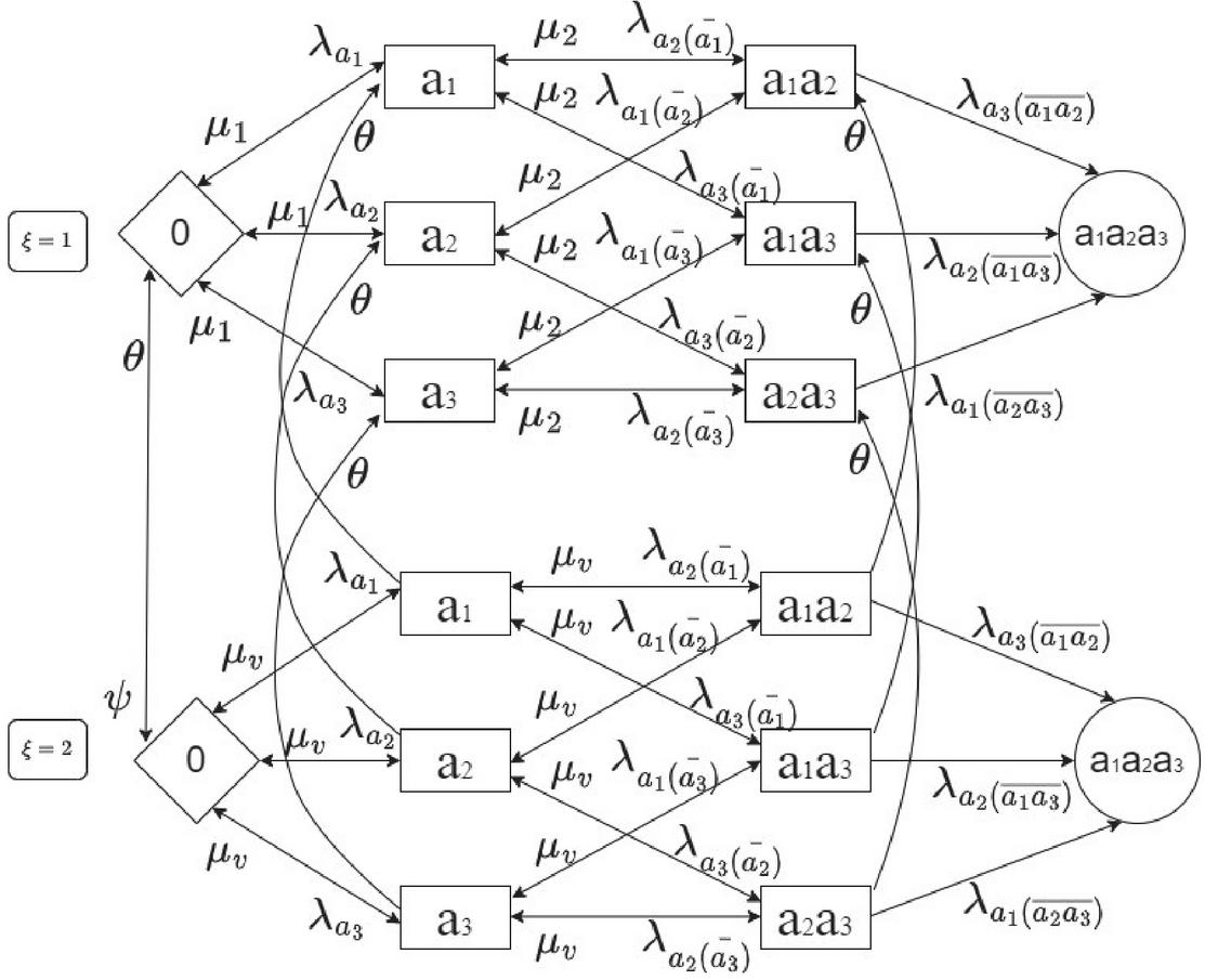
Figure 1 State transition diagram of 1-out-of-3: G system.

5.1 For $\mathit{\xi }=\mathbf{\text{1}}$

$S_0$: when no component fails in the system i.e. n=0.

case 1: all three components are working.

$S_1$: when any one component fails in the system i.e. n=1.

case 1: component 1 fails and components 2, 3 are working.

case 2: component 2 fails and components 1, 3 are working.

case 3: component 3 fails and components 1, 2 are working.

$S_2$: when any two components fail in the system i.e. n=2.

case 1: components 1, 2 fail and component 3 is working.

case 2: components 2, 3 fail and component 1 is working.

case 3: components 1, 3 fail and component 2 is working.

$S_3$: when any three components fail in the system i.e. n=3.

case 1: components 1, 2, 3 fail.

5.2 For $\mathit{\xi }=\mathbf{\text{2}}$

$S_0$: when no component fails in the system i.e. n $=$ 0.

case 1: all three components are working.

$S_1$: when any one component fails in the system i.e. n $=$ 1.

case 1: component 1 fails and components 2, 3 are working.

case 2: component 2 fails and components 1, 3 are working.

case 3: component 3 fails and components 1, 2 are working.

$S_2$: when any two components fail in the system i.e. n $=$ 2.

case 1: components 1, 2 fail and component 3 is working.

case 2: components 2, 3 fail and component 1 is working.

case 3: components 1, 3 fail and component 2 is working.

$S_3$: when any three components fail in the system i.e. n $=$ 3.

case 1: components 1, 2, 3 fail.

Now, system operational characteristics for 1-out-of-3: G system can be given as;

(a) Expected number of failed units in the system:

${\mathrm{E}}_{\mathrm{F}}(\mathrm{t})$	$=p_1^{(1)}(t)+p_2^{(1)}(t)+p_3^{(1)}(t)+2p_{1.2}^{(1)}(t)+2p_{1.3}^{(1)}(t)+2p_{2.3}^{(1)}(t)$
	$\mathrm{\hspace{1em}}+3p_{\mathrm{1.2.3}}^{(1)}(t)+p_1^{(2)}(t)+p_2^{(2)}(t)+p_3^{(2)}(t)+2p_{1.2}^{(2)}(t)$
	$\mathrm{\hspace{1em}}+2p_{1.3}^{(2)}(t)+2p_{2.3}^{(2)}(t)+3p_{\mathrm{1.2.3}}^{(2)}(t)$

(b) Expected number of standby units in the system:

${\mathrm{E}}_{\mathrm{S}}(\mathrm{t})$	$=2p_0^{(1)}(t)+p_1^{(1)}(t)+p_2^{(1)}(t)+p_3^{(1)}(t)+2p_0^{(2)}(t)$
	$\mathrm{\hspace{1em}}+p_1^{(1)}(t)+p_2^{(1)}(t)+p_3^{(1)}(t)$

(c) Probability that server is busy:

${\mathrm{P}}_{\mathrm{B}}(\mathrm{t})$	$=p_1^{(1)}(t)+p_2^{(1)}(t)+p_3^{(1)}(t)+p_4^{(1)}(t)+p_1^{(2)}(t)$
	$\mathrm{\hspace{1em}}+p_2^{(2)}(t)+p_3^{(2)}(t)+p_4^{(2)}(t)$

(d) The system reliability:

$$\mathrm{R}(\mathrm{t})=1-(p_{\mathrm{1.2.3}}^{(1)}(t)+p_{\mathrm{1.2.3}}^{(2)}(t))$$

(e) Failure frequency of the system:

$${\mathrm{W}}_{\mathrm{F}}(\mathrm{t})=\left({\lambda }_{3\left(\overline{1.2}\right)}+{\lambda }_{2\left(\overline{1.3}\right)}+{\lambda }_{1\left(\overline{2.3}\right)}\right)\left(p_{\mathrm{1.2.3}}^{(1)}(t)+p_{\mathrm{1.2.3}}^{(2)}(t)\right)$$

Illustration 2: We consider a load sharing 3-out-of-4: G system having 4 non-identical components consisting different amount of load in the proportion ${\beta }_1:{\beta }_2$:${\beta }_3:{\beta }_4$ and ${\lambda }_1,{\lambda }_2,{\lambda }_3,{\lambda }_4$ are failure rates of components 1, 2, 3 and 4 respectively. The system success states are $S_{\mathrm{n}};\mathrm{n}=0,1$ for 3-out-of-4: G system and can be defined in two stages each for two cases as:

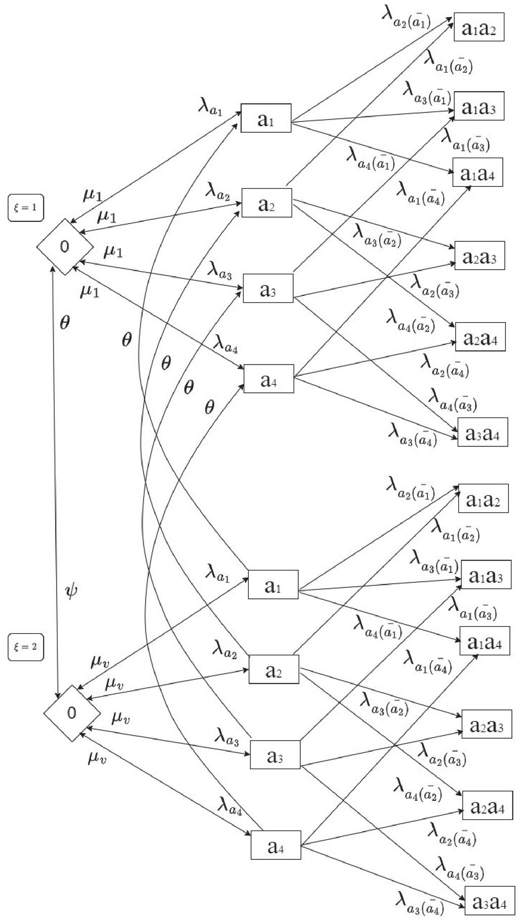
Figure 2 State transition diagram of 3-out-of-4: G system.

5.3 For $\mathit{\xi }=\mathbf{\text{1}}$

$S_0$: when no component fails in the system i.e. n $=$ 0.

case 1: all four components are working.

$S_1$: when any one component fails in the system i.e. n $=$ 1.

case 1: component 1 fails and components 2, 3, 4 are working.

case 2: component 2 fails and components 1, 3, 4 are working.

case 3: component 3 fails and components 1, 2, 4 are working.

case 4: component 4 fails and components 1, 2, 3, are working.

$S_2$: when any two components fail in the system i.e. n $=$ 2.

case 1: components 1, 2 fail and components 3, 4 are working.

case 2: components 1, 3 fail and components 2, 4 are working.

case 3: components 1, 4 fail and components 2, 3 are working.

case 4: components 2, 3 fail and components 1, 4 are working.

case 5: components 2, 4 fail and components 1, 3 are working.

case 6: components 3, 4 fail and components 1, 2 are working.

5.4 For $\mathit{\xi }=\mathbf{\text{2}}$

$S_0$: when no component fails in the system i.e. n $=$ 0.

case 1: all four components are working.

$S_1$: when any one component fails in the system i.e. n $=$ 1.

case 1: component 1 fails and components 2, 3, 4 are working.

case 2: component 2 fails and components 1, 3, 4 are working.

case 3: component 3 fails and components 1, 2, 4 are working.

case 4: component 4 fails and components 1, 2, 3, are working.

$S_2$: when any two components fail in the system i.e. n $=$ 2.

case 1: components 1, 2 fail and components 3, 4 are working.

case 2: components 1, 3 fail and components 2, 4 are working.

case 3: components 1, 4 fail and components 2, 3 are working.

case 4: components 2, 3 fail and components 1, 4 are working.

case 5: components 2, 4 fail and components 1, 3 are working.

case 6: components 3, 4 fail and components 1, 2 are working.

Particularly, system operational characteristics for 3-out-of-4: G redundant-system can be written as;

(a) Expected number of failed units in the system:

$${\mathrm{E}}_{\mathrm{F}}(\mathrm{t})=\sum _{\mathrm{i}=1}^2\sum _{lϵS_i}i{p}_l^{(1)}(\mathrm{t})+\sum _{\mathrm{i}=1}^2\sum _{lϵS_i}i{p}_l^{(2)}(\mathrm{t})$$

(b) Expected number of standby units in the system:

$${\mathrm{E}}_{\mathrm{S}}(\mathrm{t})=\sum _{lϵS_0}{p}_l^{(1)}(\mathrm{t})+\sum _{lϵS_0}{p}_l^{(2)}(\mathrm{t})$$

(c) Probability that server is busy:

$${\mathrm{P}}_{\mathrm{B}}(\mathrm{t})=\sum _{\mathrm{i}=1}^2\sum _{lϵS_i}{p}_l^{(1)}(\mathrm{t})+\sum _{\mathrm{i}=1}^2\sum _{lϵS_i}{p}_l^{(2)}(\mathrm{t})$$

(d) The system reliability:

$$\mathrm{R}(\mathrm{t})=1-\left(\sum _{lϵS_2}{p}_l^{(1)}(\mathrm{t})+\sum _{lϵS_2}{p}_l^{(2)}(\mathrm{t})\right)$$

(e) Failure frequency of the system:

${\mathrm{W}}_{\mathrm{F}}(\mathrm{t})$	$=({\lambda }_{2(\overline{1})}+{\lambda }_{1(\overline{2})})(p_{1.2}^{(1)}(t)+p_{1.2}^{(2)}(t))+({\lambda }_{3(\overline{1})}+{\lambda }_{1(\overline{3})})(p_{1.3}^{(1)}(t)$
	$\mathrm{\hspace{1em}}+p_{1.3}^{(2)}(t))+({\lambda }_{4(\overline{1})}+{\lambda }_{1(\overline{4})})(p_{1.4}^{(1)}(t)+p_{1.4}^{(2)}(t))$
	$\mathrm{\hspace{1em}}+({\lambda }_{3(\overline{2})}+{\lambda }_{2(\overline{3})})(p_{2.3}^{(1)}(t)+p_{2.3}^{(2)}(t))$
	$\mathrm{\hspace{1em}}+({\lambda }_{4(\overline{2})}+{\lambda }_{2(\overline{4})})(p_{2.4}^{(1)}(t)+p_{2.4}^{(2)}(t))$
	$\mathrm{\hspace{1em}}+({\lambda }_{4(\overline{3})}+{\lambda }_{4(\overline{3})})(p_{3.4}^{(1)}(t)+p_{3.4}^{(2)}(t))$

6 Numerical Simulation

In this section, we explore now numerical simulation of different performance measures for variability of the parameters which are simulated on above two illustrations. MATLAB software is used for this purpose. For 1-out-of-3: G system, we set the following default parameters: ${\lambda }_1=0.5,{\lambda }_2=0.3,{\lambda }_3=0.1,{\lambda }_{\mathrm{c}}=0.5,\mathrm{M}=2,\delta =1,{\beta }_1=0.2,{\beta }_2=0.3,{\beta }_3=0.1,{\mu }_1=0.3,{\mu }_2=0.1,\theta =0.01,{\mathrm{V}}_1=1,{\mathrm{V}}_2=2$ and $\phi =0.2$. For 3-out-of-4: G system we set the default parameters as follows: ${\lambda }_1=0.5,{\lambda }_2=0.3,{\lambda }_3=0.1,{\lambda }_4=0.001,{\lambda }_{\mathrm{c}}=0.1,\mathrm{M}=1,\delta =1,{\beta }_1=0.2,{\beta }_2=0.3,{\beta }_3=0.1,{\beta }_4=4,{\mu }_1=0.3,\theta =1,{\mathrm{V}}_1=1$ and $\phi =0.2$.

The numerical results of the system reliability, other operational characteristics are summarized in Figures 3–6 and Tables 2 and 3. Moreover, the cost-estimation of both illustrations can be visualized in Figures 7–11. We also compare cost results with neuro-fuzzy results determined from fuzzy toolbox of MATLAB package.

In Figures 3–6, we display the effect of the system reliability with respect to time ‘t’ by varying parameters ${\lambda }_{\mathrm{c}},{\mu }_1,\delta$ and ${\beta }_1$ respectively. In these figures, we can see a gradual decrease in system reliability with respect to the time and then it becomes asymptotically constant. From Figures 1(i) and 1(ii), we observe that the reliability of 1-out-of-3: G and 3-out-of-4: G systems decrease significantly as common cause failure rate $({\lambda }_{\mathrm{c}})$ increase. Figures 4(i) and 4(ii) show that the reliability of both systems achieves higher values with the increment in repair rate $({\mu }_1)$.

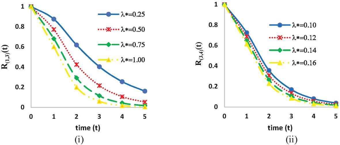
Figure 3 Reliability v/s time by varying ${\lambda }_{\mathrm{c}}=\lambda *$ for (i) 1-out-of-3: G system and (ii) 3-out-of-4: G system.

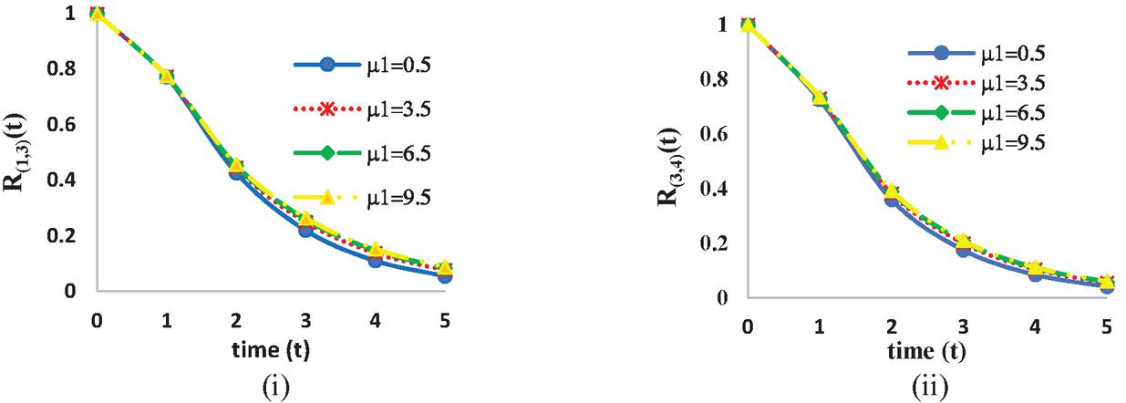
Figure 4 Reliability v/s time by varying ${\mu }_1$ for (i) 1-out-of-3: G system and (ii) 3-out-of-4: G system.

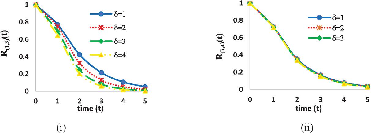
Figure 5 Reliability v/s time by varying $\delta$ system for (i) 1-out-of-3: G system and (ii) 3-out-of-4: G system.

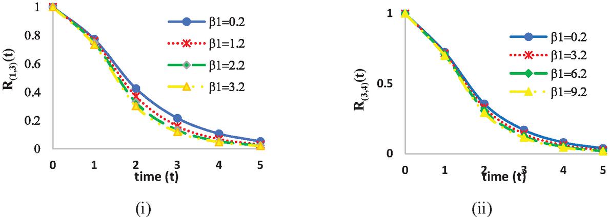
Figure 6 Reliability v/s time by varying ${\beta }_1$ for (i) 1-out-of-3: G system and (ii) 3-out-of-4: G system.

Table 2 Performance indices of 1-out-of-3: G system

Indices of 1-out-of-3 System
Indices	${\mu }_1=0.3$	${\mu }_1=1.3$
$\downarrow$	t $=$ 0	t $=$ 1	t $=$ 2	t $=$ 3	t $=$ 4	t $=$ 0	t $=$ 1	t $=$ 2	t $=$ 3	t $=$ 4
$E_F(t)$	0	0.9846	2.0756	2.5653	2.7904	0	0.9342	1.9618	2.4678	2.7233
$E_S(t)$	1	0.514	0.1664	0.0672	0.0313	1	0.5576	0.2399	0.116	0.0586
A$(t)$	1	0.6718	0.3081	0.1449	0.0699	1	0.6886	0.3461	0.1774	0.0922
$P_B(t)$	0	0.486	0.8336	0.9328	0.9687	0	0.4424	0.7601	0.884	0.9414
$P_V(t)$	0	0.0694	0.119	0.1322	0.1357	0	0.0712	0.1334	0.157	0.1661
$W_F(t)$	0	0.6132	1.5516	2.116	2.4121	0	0.6116	1.5269	2.0728	2.3697
Indices	$V_1=1$	$V_1=2$
$\downarrow$	t $=$ 0	t $=$ 1	t $=$ 2	t $=$ 3	t $=$ 4	t $=$ 0	t $=$ 1	t $=$ 2	t $=$ 3	t $=$ 4
$E_F(t)$	0	0.9846	2.0756	2.5653	2.7904	0	0.9831	2.0678	2.5561	2.7827
$E_S(t)$	1	0.514	0.1664	0.0672	0.0313	1	0.5154	0.1729	0.0743	0.0367
A$(t)$	1	0.6718	0.3081	0.1449	0.0699	1	0.6723	0.3107	0.148	0.0724
$P_B(t)$	0	0.486	0.8336	0.9328	0.9687	0	0.4846	0.8271	0.9257	0.9633
$P_V(t)$	0	0.0694	0.119	0.1322	0.1357	0	0.0694	0.119	0.1323	0.1359
$W_F(t)$	0	0.6132	1.5516	2.116	2.4121	0	0.6132	1.5509	2.1142	2.4099
Indices	${\lambda }_c=0.3$	${\lambda }_c=1.3$
$\downarrow$	t $=$ 0	t $=$ 1	t $=$ 2	t $=$ 3	t $=$ 4	t $=$ 0	t $=$ 1	t $=$ 2	t $=$ 3	t $=$ 4
$E_F(t)$	0	0.9846	2.0756	2.5653	2.7904	0	1.7776	2.7937	2.9643	2.9937
$E_S(t)$	1	0.514	0.1664	0.0672	0.0313	1	0.3118	0.0371	0.0055	0.0009
A$(t)$	1	0.6718	0.3081	0.1449	0.0699	1	0.4075	0.0688	0.0119	0.0021
$P_B(t)$	0	0.486	0.8336	0.9328	0.9687	0	0.6882	0.9629	0.9945	0.9991
$P_V(t)$	0	0.0694	0.119	0.1322	0.1357	0	0.0563	0.0772	0.0786	0.0781
$W_F(t)$	0	0.6132	1.5516	2.116	2.4121	0	1.4343	2.4438	2.6521	2.6913
Indices	${\lambda }_1=0.3$	${\lambda }_1=1.3$
$\downarrow$	t $=$ 0	t $=$ 1	t $=$ 2	t $=$ 3	t $=$ 4	t $=$ 0	t $=$ 1	t $=$ 2	t $=$ 3	t $=$ 4
$E_F(t)$	0	0.9846	2.0756	2.5653	2.7904	0	1.2837	2.4002	2.7733	2.9092
$E_S(t)$	1	0.514	0.1664	0.0672	0.0313	1	0.3252	0.0563	0.0167	0.0067
A$(t)$	1	0.6718	0.3081	0.1449	0.0699	1	0.5721	0.1999	0.0756	0.0303
$P_B(t)$	0	0.486	0.8336	0.9328	0.9687	0	0.6748	0.9437	0.9833	0.9933
$P_V(t)$	0	0.0694	0.119	0.1322	0.1357	0	0.0569	0.0806	0.0837	0.0839
$W_F(t)$	0	0.6132	1.5516	2.116	2.4121	0	1.1356	3.0251	4.0045	4.4182
Indices	${\beta }_2=0.3$	${\beta }_2=1.3$
$\downarrow$	t $=$ 0	t $=$ 1	t $=$ 2	t $=$ 3	t $=$ 4	t $=$ 0	t $=$ 1	t $=$ 2	t $=$ 3	t $=$ 4
$E_F(t)$	0	0.9846	2.0756	2.5653	2.7904	0	1.0163	2.1443	2.6177	2.8227
$E_S(t)$	1	0.514	0.1664	0.0672	0.0313	1	0.513	0.1626	0.0638	0.0288
A$(t)$	1	0.6718	0.3081	0.1449	0.0699	1	0.6612	0.2852	0.1274	0.0591
$P_B(t)$	0	0.486	0.8336	0.9328	0.9687	0	0.487	0.8374	0.9362	0.9712
$P_V(t)$	0	0.0694	0.119	0.1322	0.1357	0	0.0694	0.1185	0.1312	0.1345
$W_F(t)$	0	0.6132	1.5516	2.116	2.4121	0	1.429	3.7028	4.9057	6.320

Table 3 Performance indices of 3-out-of-4: G system

Indices of 3-out-of-4 System
Indices	${\lambda }_c=0.1$	${\lambda }_c=0.2$
$\downarrow$	t $=$ 0	t $=$ 1	t $=$ 2	t $=$ 3	t $=$ 4	t $=$ 0	t $=$ 1	t $=$ 2	t $=$ 3	t $=$ 4
$E_F(t)$	0	0.7848	1.494	1.7715	1.8936	0	1.0842	1.7635	1.9294	1.9778
$E_S(t)$	1	0.4901	0.1493	0.0579	0.0253	1	0.3638	0.0639	0.0156	0.0045
A$(t)$	1	0.6076	0.253	0.1142	0.0532	1	0.4579	0.1182	0.0353	0.0111
$P_B(t)$	0	0.5099	0.8507	0.9421	0.9747	0	0.6362	0.9361	0.9844	0.9955
$P_V(t)$	0	0.0521	0.0476	0.027	0.0139	0	0.0454	0.033	0.0154	0.0065
$W_F(t)$	0	0.3743	0.8237	1.04	1.143	0	0.631	1.128	1.2763	1.3232
Indices	${\lambda }_1=0.3$			${\lambda }_1=1.3$
$\downarrow$	t $=$ 0	t $=$ 1	t $=$ 2	t $=$ 3	t $=$ 4	t $=$ 0	t $=$ 1	t $=$ 2	t $=$ 3	t $=$ 4
$E_F(t)$	0	0.7848	1.494	1.7715	1.8936	0	1.0146	1.6896	1.8881	1.9581
$E_S(t)$	1	0.4901	0.1493	0.0579	0.0253	1	0.3122	0.0562	0.0172	0.0062
A$(t)$	1	0.6076	0.253	0.1142	0.0532	1	0.4927	0.1552	0.0559	0.021
$P_B(t)$	0	0.5099	0.8507	0.9421	0.9747	0	0.6878	0.9438	0.9828	0.9938
$P_V(t)$	0	0.0521	0.0476	0.027	0.0139	0	0.042	0.0292	0.0139	0.0062
$W_F(t)$	0	0.3743	0.8237	1.04	1.143	0	0.8831	1.9218	2.3196	2.4685
Indices	${\mu }_1$=0.3	${\mu }_1$=1.3
$\downarrow$	t $=$ 0	t $=$ 1	t $=$ 2	t $=$ 3	t $=$ 4	t $=$ 0	t $=$ 1	t $=$ 2	t $=$ 3	t $=$ 4
$E_F(t)$	0	0.7848	1.494	1.7715	1.8936	0	0.7373	1.4003	1.7008	1.8498
$E_S(t)$	1	0.4901	0.1493	0.0579	0.0253	1	0.5356	0.2307	0.1137	0.057
A$(t)$	1	0.6076	0.253	0.1142	0.0532	1	0.6313	0.2998	0.1496	0.0751
$P_B(t)$	0	0.5099	0.8507	0.9421	0.9747	0	0.4644	0.7693	0.8863	0.943
$P_V(t)$	0	0.0521	0.0476	0.027	0.0139	0	0.0537	0.0573	0.0383	0.0227
$W_F(t)$	0	0.3743	0.8237	1.04	1.143	0	0.3749	0.8332	1.064	1.1801
Indices	$V_1$=1	$V_1$=2
$\downarrow$	t $=$ 0	t $=$ 1	t $=$ 2	t $=$ 3	t $=$ 4	t $=$ 0	t $=$ 1	t $=$ 2	t $=$ 3	t $=$ 4
$E_F(t)$	0	0.7848	1.494	1.7715	1.8936	0	0.7838	1.4906	1.7689	1.8921
$E_S(t)$	1	0.4901	0.1493	0.0579	0.0253	1	0.4911	0.1524	0.06	0.0264
A$(t)$	1	0.6076	0.253	0.1142	0.0532	1	0.6081	0.2547	0.1155	0.054
$P_B(t)$	0	0.5099	0.8507	0.9421	0.9747	0	0.5089	0.8476	0.94	0.9736
$P_V(t)$	0	0.0521	0.0476	0.027	0.0139	0	0.0521	0.0477	0.0272	0.014
$W_F(t)$	0	0.3743	0.8237	1.04	1.143	0	0.3743	0.8239	1.0408	1.1443
Indices	${\beta }_4=1$	${\beta }_4=4$
$\downarrow$	t $=$ 0	t $=$ 1	t $=$ 2	t $=$ 3	t $=$ 4	t $=$ 0	t $=$ 1	t $=$ 2	t $=$ 3	t $=$ 4
$E_F(t)$	0	0.7848	1.494	1.7715	1.8936	0	0.7875	1.5019	1.7789	1.8986
$E_S(t)$	1	0.4901	0.1493	0.0579	0.0253	1	0.49	0.1484	0.0568	0.0244
A$(t)$	1	0.6076	0.253	0.1142	0.0532	1	0.6062	0.249	0.1106	0.0507
$P_B(t)$	0	0.5099	0.8507	0.9421	0.9747	0	0.51	0.8516	0.9432	0.9756
$P_V(t)$	0	0.0521	0.0476	0.027	0.0139	0	0.0521	0.0475	0.0269	0.0137
$W_F(t)$	0	0.2127	0.5116	0.6631	0.7345	0	0.3743	0.8237	1.04	1.143

Figures 5(i–ii) and 6(i–ii), depict the trend of reliability of systems for different values of parameters $\delta$ and ${\beta }_1$, respectively. Figure 5(i) shows that R(t) decreases by enhancing $\delta$ for 1-out-of-3: G system whereas, no significant effect of $\delta$ in Figure 5(ii) cannot be obtained in the reliability R(t) of 3-out-of-4: G system. Figures 6(i) and 6(ii) show that the reliability of both system decreases by enhancing ${\beta }_1$.

In Tables 2 and 3, we observe that ${\mathrm{E}}_{\mathrm{F}}(\mathrm{t}),{\mathrm{P}}_{\mathrm{B}}(\mathrm{t}),{\mathrm{P}}_{\mathrm{V}}(\mathrm{t})$ and ${\mathrm{W}}_{\mathrm{F}}(\mathrm{t})$ increase with the increase in time (t) whereas ${\mathrm{E}}_{\mathrm{S}}(\mathrm{t})$ and $A(\mathrm{t})$ decrease as time (t) grows. Further, it is examined that the indices ${\mathrm{E}}_{\mathrm{F}}(\mathrm{t}),{\mathrm{P}}_{\mathrm{B}}(\mathrm{t})$ and ${\mathrm{W}}_{\mathrm{F}}(\mathrm{t})$ decrease on enhancing the values of ${\mu }_1$ and ${\mathrm{V}}_1$; on a contrary these measures increase for decreasing values of ${\lambda }_{\mathrm{c}},{\lambda }_1$ and ${\beta }_2/{\beta }_4$ (see Tables 2 and 3).

In this way, reverse pattern of indices ${\mathrm{E}}_{\mathrm{S}}(\mathrm{t}),\mathrm{A}(\mathrm{t})$ and ${\mathrm{P}}_{\mathrm{V}}(\mathrm{t})$ could be noticed for parameters ${\mu }_1,{\mathrm{V}}_1,{\lambda }_{\mathrm{c}},{\lambda }_1$ and ${\beta }_2/{\beta }_4$ (see in Tables 2 and 3).

Table 4 The cost parameters for two different sets

Cost in $	${\mathrm{C}}_{\mathrm{F}}$	${\mathrm{C}}_{\mathrm{S}}$	${\mathrm{C}}_{\mathrm{B}}$	${\mathrm{C}}_{\mathrm{V}}$
Set 1	30	120	50	150
Set 2	30	125	50	140

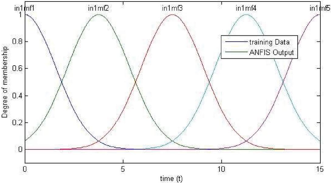
Figure 7 Membership function for time (t).

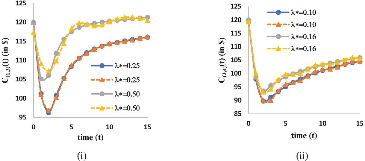
Figure 8 Cost v/s time by varying ${\lambda }_{\mathrm{c}}=\lambda *$ for cost set 1 for (i) 1-out-of-3: G system and (ii) 3-out-of-4: G system.

Figure 9 Cost v/s time by varying $\theta$ for cost set 1 for (i) 1-out-of-3: G system and (ii) 3-out-of-4: G system.

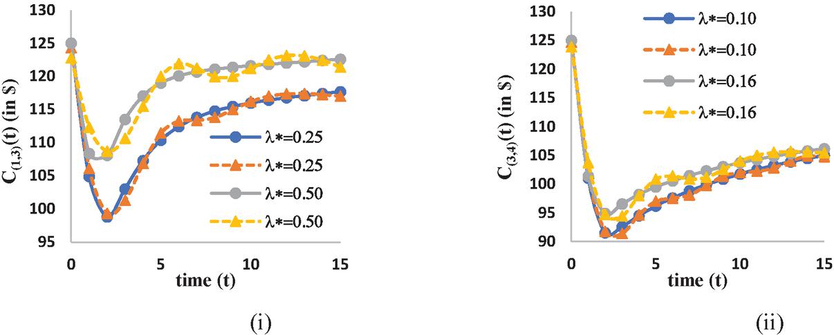
Figure 10 Cost v/s time by varying ${\lambda }_c=\lambda *$ for cost set 2 for (i) 1-out-of-3: G system and (ii) 3-out-of-4: G system.

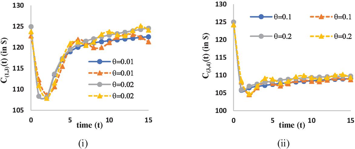
Figure 11 Cost v/s time by varying $\theta$ for cost set 2 for (i) 1-out-of-3: G system and (ii) 3-out-of-4: G system.

The numerical results to examine the behavior of total system cost with respect to time in neuro-fuzzy environment are summarized in Figures 7–11. We consider two sets of unit costs for both the systems 1-out-of-3: G and 3-out-of-4: G, as given in Table 4. The membership function for input-parameter time (t) is described by gaussian distribution in Figure 7. In Figures 8–11, the continuous lines show analytical results whereas doted lines represent artificial neuro fuzzy inference system (ANFIS) based numerical results.

• For cost set-I; Figures 8(i–ii) and 9(i–ii) depict the system total cost with respect to time for different values of ${\lambda }_{\mathrm{c}}$ (see Figure 8) and $\theta$ (see Figure 9) for 1-out-of-3: G system and 3-out-of-4: G systems. In Figures 8(i–ii) and 9(i–ii), there is steep decrease in total cost for lower values of time t, and then it starts to increase gradually, until it attains an asymptotic constant value. We notice that the predicted total cost increase as the value of ${\lambda }_{\mathrm{c}}$ and $\theta$ increase.

• For cost set-II; Figures 10(i–ii) and 11(i–ii) are examined to see the effect of total system cost with respect to time (t) for different values of ${\lambda }_{\mathrm{c}}$ and $\theta$, respectively. We see that total cost of the system first decreases sharply, after getting optimal value it become shows asymptotically increasing pattern and it shows significant increment. The effect of system total cost varying parameters ${\lambda }_{\mathrm{c}}$ and $\theta ,$ is similar as we examined in Figures 8 and 9 respectively.

The following results are observed on the in-depth qualitative and optimal study:

• Regular maintenance of the system is recommended to prevent unit/system failure which has a direct impact on the system performance.

• The repair rate increases, the reliability of the load-sharing K-out-of-N: G system increases. On the contrary, reliability varies significantly in relation to various parameters e.g. failure rates of operating and standby units. The reliability decreases for higher values of failure rates of operating and standby units.

• The reliability of K-out-of-N: G system is very sensitive with respect to parameter of mean failure/repair, but result is found less remarkable for load sensitivity.

• Working vacation is critical component of sustaining a high level of service. As a preventative precaution, the appropriate server vacation rate should be preserved to avoid idle time or additional service costs.

• The tractability of ANFIS results for analysing the system cost has benefitted to establish best fitted comparison with numerical results that match with real life scenarios.

• The proposed reliability assessment characterizes load sharing systems with non-identical components with sensitivity of parameters. Sometimes component failure cannot be controlled, and system may prone to failure. In this point of view, sensitivity analysis of parameters may provide an effective support for decision makers to maintain the reliability for desired levels and to obtain expected number of failed operating/standby components along with the cost of the model which is advantageous to system designers and production engineers in techno-economic sense.

7 Conclusion

The Markovian analysis for the load sharing K-out-of-N: G repairable machining system with the support of non-identical repairable components and common cause failure has been investigated in this paper. The repair provision and working vacation concepts were introduced to analyze real-time repairable system wherein the failed components get immediately repaired by the server (if not on vacation) and unequal load is distributed among remaining surviving components. To determine the transient system probabilities, Chapman Kolmogorov equations were developed and solved using Runge-Kutta method. We have provided the explicit expressions to obtain the system reliability and various average operational indices along with the system cost estimate. The numerical results have been carried out for comparative and optimal analysis of system reliability and cost by taking illustrations. The model can be utilized in a variety of machining systems in a variety of industries, including software and hardware systems, power generation, power plants, communications, among others. The findings could aid production engineers and system designers in improving the reliability of load-sharing systems with component failure dependencies. The current analysis could be extended to include switching failure, standby facing independent failure, additional repairmen, unreliable server, a K-out-of-(P+N): G repairable system with different type of components and more realistic policies such as a N, T or D policy into the current study to improve model insight for coping with a more realistic scenario.

Acknowledgements

The author (Sudeep Kumar) is appreciative to CSIR (council of scientific and industrial research), Delhi for financial support (File No. 09/915(0018)/2019-EMR-I). The authors greatly acknowledge the Associate Editor’s and learned referees’ critical comments and suggestions, which considerably help us in improving this research.

References

[1] S. Eryilmaz, ‘On reliability analysis of a k-out-of-n system with components having random weights’, Reliab. Eng. Syst. Saf., vol. 109, pp. 41–44, Jan. 2013, doi: 10.1016/j.ress.2012.07.010. https://www.sciencedirect.com/science/article/pii/S0951832012001615

[2] Y. Mo, L. Xing, S. V. Amari, and J. Bechta Dugan, ‘Efficient analysis of multi-state k-out-of-n systems’, Reliab. Eng. Syst. Saf., vol. 133, pp. 95–105, Jan. 2015, doi: 10.1016/j.ress.2014.09.006. https://www.sciencedirect.com/science/article/pii/S0951832014002166

[3] T. Yuge, M. Maruyama, and S. Yanagi, ‘Reliability of a k-out-of-n System with Common-cause Failures Using Multivariate Exponential Distribution’, Procedia Comput. Sci., vol. 96, pp. 968–976, Jan. 2016, doi: 10.1016/j.procs.2016.08.101. https://www.sciencedirect.com/science/article/pii/S1877050916318920

[4] R. A. Rahmani, M. Izadi, and B. E. Khaledi, ‘Importance of components in k-out-of-n system with components having random weights’, J. Comput. Appl. Math., vol. 296, pp. 1–9, Apr. 2016, doi: 10.1016/j.cam.2015.09.009. https://www.sciencedirect.com/science/article/pii/S0377042715004616

[5] J. E. Byun, H. M. Noh, and J. Song, ‘Reliability growth analysis of k-out-of-N systems using matrix-based system reliability method’, Reliab. Eng. Syst. Saf., vol. 165, pp. 410–421, Sep. 2017, doi: 10.1016/j.ress.2017.05.001. https://www.semanticscholar.org/paper/Reliability-growth-analysis-of-k-out-of-N-systems-Byun-Noh/c36ced21189d2f2e693db436c9ca003bbe39ce8a

[6] K. O. Kim, ‘Optimal number of components in a load-sharing system for maximizing reliability’, J. Korean Stat. Soc., vol. 47, no. 1, pp. 32–40, Mar. 2018, doi: 10.1016/j.jkss.2017.08.003. https://www.sciencedirect.com/science/article/abs/pii/S1226319217300583

[7] E. Nezakati and M. Razmkhah, ‘Reliability analysis of a load sharing k-out-of-n:F degradation system with dependent competing failures’, Reliab. Eng. Syst. Saf., vol. 203, p. 107076, Nov. 2020, doi: 10.1016/j.ress.2020.107076. https://www.sciencedirect.com/science/article/pii/S0951832020305779

[8] A. Dembinska, N. I. Nikolov, and E. Stoimenova, ‘Reliability properties of k-out-of-n systems with one cold standby unit’, J. Comput. Appl. Math., vol. 388, p. 113289, May 2021, doi: 10.1016/j.cam.2020.113289. https://www.sciencedirect.com/science/article/abs/pii/S037704272030580X

[9] K. Jenab and B. S. Dhillon, ‘Assessment of reversible multi-state k-out-of-n:G/F/Load-Sharing systems with flow-graph models’, Reliab. Eng. Syst. Saf., vol. 91, no. 7, pp. 765–771, Jul. 2006, doi: 10.1016/j.ress.2005.07.003. https://www.sciencedirect.com/science/article/abs/pii/S095183200500147X

[10] T. Yinghui and Z. Jing, ‘New model for load-sharing k-out-of-n: G system with different components’, J. Syst. Eng. Electron., vol. 19, no. 4, pp. 748–842, Aug. 2008, doi: 10.1016/S1004-4132(08)60148-6. https://www.sciencedirect.com/science/article/abs/pii/S1004413208601486

[11] W. Yamamoto, L. Jin, and K. Suzuki, ‘Optimal allocations for load-sharing k-out-of-n:F systems’, J. Stat. Plan. Inference, vol. 139, no. 5, pp. 1777–1781, May 2009, doi: 10.1016/j.jspi.2008.05.029. https://www.sciencedirect.com/science/article/abs/pii/S0378375808002528

[12] J. V. Deshpande, I. Dewan, and U. V. Naik-Nimbalkar, ‘A family of distributions to model load sharing systems’, J. Stat. Plan. Inference, vol. 140, no. 6, pp. 1441–1451, Jun. 2010, doi: 10.1016/j.jspi.2009.12.005. https://www.sciencedirect.com/science/article/abs/pii/S0378375809003759

[13] B. Singh and P. K. Gupta, ‘Load-sharing system model and its application to the real data set’, Math. Comput. Simul., vol. 82, no. 9, pp. 1615–1629, May 2012, doi: 10.1016/j.matcom.2012.02.010. https://www.sciencedirect.com/science/article/pii/S0378475412000699

[14] H. Z. Abou-Ziyan and A. F. Alajmi, ‘Effect of load-sharing operation strategy on the aggregate performance of existed multiple-chiller systems’, Appl. Energy, vol. 135, pp. 329–338, Dec. 2014, doi: 10.1016/j.apenergy.2014.06.065. https://www.sciencedirect.com/science/article/pii/S0306261914006473

[15] N. Zhang, M. Fouladirad, and A. Barros, ‘Maintenance analysis of a two-component load-sharing system’, Reliab. Eng. Syst. Saf., vol. 167, pp. 67–74, Nov. 2017, doi: 10.1016/j.ress.2017.05.027. https://www.sciencedirect.com/science/article/pii/S0951832016302344

[16] J. Zhang, Y. Zhao, and X. Ma, ‘Reliability modeling methods for load-sharing k-out-of-n system subject to discrete external load’, Reliab. Eng. Syst. Saf., vol. 193, p. 106603, Jan. 2020, doi: 10.1016/j.ress.2019.106603. https://www.sciencedirect.com/science/article/pii/S0951832019302145

[17] Y. Zhang, ‘Reliability Analysis of Randomly Weighted k-out-of-n Systems with Heterogeneous Components’, Reliab. Eng. Syst. Saf., vol. 205, p. 107184, Jan. 2021, doi: 10.1016/j.ress.2020.107184. https://www.sciencedirect.com/science/article/pii/S0951832020306852

[18] R. Gupta and Z. Tasneem, ‘Load sharing repairable system with imperfect coverage in fuzzy environment’, Int. J. Qual. Reliab. Manag., vol. 39, no. 7, pp. 1725–1744, Feb. 2022, doi: 10.1108/IJQRM-08-2021-0298. https://www.emerald.com/insight/content/doi/10.1108/IJQRM-08-2021-0298/full/html

[19] C. H. Lin and J. C. Ke, ‘Multi-server system with single working vacation’, Appl. Math. Model., vol. 33, no. 7, pp. 2967–2977, Jul. 2009, doi: 10.1016/j.apm.2008.10.006. https://sci-hub.se/10.1016/j.apm.2008.10.006

[20] L. Yuan and Z. D. Cui, ‘Reliability analysis for the consecutive-k-out-of-n: F system with repairmen taking multiple vacations’, Appl. Math. Model., vol. 37, no. 7, pp. 4685–4697, Apr. 2013, doi: 10.1016/j.apm.2012.09.008. https://www.sciencedirect.com/science/article/pii/S0307904X12005057

[21] W. Wu, Y. Tang, M. Yu, and Y. Jiang, ‘Reliability analysis of a k-out-of-n:G repairable system with single vacation’, Appl. Math. Model., vol. 38, no. 24, pp. 6075–6097, Dec. 2014, doi: 10.1016/j.apm.2014.05.020. https://www.sciencedirect.com/science/article/pii/S0307904X14002820

[22] M. Habib, F. Yalaoui, H. Chehade, N. Chebbo, and I. Jarkass, ‘Design optimization and redundant dependency study of series k-out-of-n: G repairable systems’, IFAC-Papers On Line, Jan. 2016, vol. 49, no. 28, pp. 126–131, doi: 10.1016/j.ifacol.2016.11.022. https://www.sciencedirect.com/science/article/pii/S2405896316324466

[23] H. Kim, ‘Optimal reliability design of a system with k-out-of-n subsystems considering redundancy strategies’, Reliab. Eng. Syst. Saf., vol. 167, pp. 572–582, Nov. 2017, doi: 10.1016/j.ress.2017.07.004. https://www.sciencedirect.com/science/article/pii/S0951832017300959

[24] Y. Zhang, W. Wu, and Y. Tang, ‘Analysis of an k-out-of-n:G system with repairman’s single vacation and shut off rule’, Oper. Res. Perspect., vol. 4, pp. 29–38, 2017, doi: 10.1016/j.orp.2017.02.002. https://www.sciencedirect.com/science/article/pii/S2214716016301002

[25] D. Y. Yang and C. L. Tsao, ‘Reliability and availability analysis of standby systems with working vacations and retrial of failed components’, Reliab. Eng. Syst. Saf., vol. 182, pp. 46–55, Feb. 2019, doi: 10.1016/j.ress.2018.09.020. https://www.sciencedirect.com/science/article/pii/S0951832018303302

[26] C. Shekhar, A. Kumar, and S. Varshney, ‘Load sharing redundant repairable systems with switching and reboot delay’, Reliab. Eng. Syst. Saf., vol. 193, p. 106656, Jan. 2020, doi: 10.1016/j.ress.2019.106656. https://www.sciencedirect.com/science/article/pii/S0951832019305174

[27] C. Wu, R. Pan, X. Zhao, and S. Cao, ‘Reliability evaluation of consecutive-k-out-of-n: F systems with two performance sharing groups’, Comput. Ind. Eng., vol. 153, p. 107092, Mar. 2021, doi: 10.1016/j.cie.2020.107092. https://www.sciencedirect.com/science/article/pii/S0360835220307622

[28] M. Jain and R. Gupta, ‘Load sharing M-out of-N: G system with non-identical components subject to common cause failure’, Int. J. Math. Oper. Res., vol. 4, no. 5, pp. 586–605, 2012, doi: 10.1504/IJMOR.2012.048932. https://www.inderscienceonline.com/doi/abs/10.1504/IJMOR.2012.048932

Biographies

Sudeep Kumar has received his MSc degree in 2017. He is presently conducting research leading to PhD Degree in the Department of Mathematics, Amity Institute of Applied Science, Amity University, Noida, India. He has attended and presented his work in International and National conferences/seminars. His areas of interest are software and hardware reliability and performance analysis of machine repair problems.

Ritu Gupta is faculty in Department of Mathematics, Amity University, Noida, India. She received Ph.D. degree from Department of Mathematics, Institute of Basic Science, Dr. B. R. Ambedkar University, Agra, India. She has published several research papers in reputed journals/refereed proceedings. She has attended and presented her work in twenty-five International and National Conferences/Seminars. Her areas of interest are reliability modeling of software/hardware systems, performance modeling of fault tolerant systems, machine repairing systems and queueing problems.

Journal of Reliability and Statistical Studies, Vol. 15, Issue 2 (2022), 583–616.
doi: 10.13052/jrss0974-8024.1528
© 2022 River Publishers