The Bayesian Reliability Analysis of the Alpha Power Gompertz Model

Joseph Thomas Eghwerido^1,* Suraju Olaniyi Ogundele¹, Lawrence Chukwudumebi Nzei² and Friday Ikechukwu Agu³

¹Department of Statistics, Federal University of Petroleum Resources, Effurun, Delta State, Nigeria
²Department of Statistics, University of Benin, Edo State, Nigeria
³Department of Statistics, University of Calabar, Cross-River State, Nigeria
E-mail: eghwerido.joseph@fupre.edu.ng
*Corresponding Author

Received 03 October 2020; Accepted 09 August 2022; Publication 28 September 2022

Abstract

This article introduced the determination of reliability analysis of the alpha power Gompertz model using the Bayesian techniques. The method developed has been evaluated using women breast cancer in the Stan implementation in R. A survival data used illustrates the proposed Bayesian approach.

Keywords: Bayesian inference, posterior, prior, regression analysis, rstan package, simulation.

1 Introduction

Modeling survival time in an event has received attention recently. This may be due to an upsurge in data analyses and their applications. However, modeling survival time in events depends on the statistical distributions. Thus, there is a need to developed a model that represents the true characteristics of the survival datasets. In statistical distribution, most newly developed traditional distributions do not characterised the true characteristics of the data set. However, to improve these distributions, families of statistical distributions are being developed to extend, make adequate, and improve existing traditional distributions. One of such all times classical distribution is the Gompertz distribution.

The Gompertz distribution is a continuous probability distribution named after the author Benjamin Gompert. The Gompertz distribution is often applied to describe the distribution of adult lifespans and more recently, it has been applied to failure rates of computer code. The Gompertz distribution has exponentially increasing failure rate. Thus, a monotonic increasing survival rate function are used to describe survival rates in epidemiology, biology, chemistry, engineering, hydrology, gerontology, public health, and economics. Thus, because of its all inclusions applications, there is need to modify the Gompertz model to represent the true nature of the applied data set. The alpha power Gompertz distribution proposed by Eghwerido et al. 2020 has found its tractability, simplicity, applicability and flexibility in classical statistical literature.

A number of distinct Bayesian models have been proposed in existing literature researched. [14] presented the Marshall-Olkin one-parameter transformation. [1] proposed the Bayesian analysis of the Marshall-Olkin model with special attention to exponential, exponentiated exponential and exponential extension. [2] proposed the Bayesian survival analysis of the type I generalized exponential model. [5] proposed the Bayesian analysis of the generalized log-Burr family of distribution. [3] proposed the Bayesian analysis with Stan with emphasis on the exponential model. [8] proposed the Bayesian method of analysis for data analysis. [4] proposed a Bayesian analysis of the Topp-Leone generalized model. [19] obtained the unimodal density using the Bernstein polynomials. [15] proposed the Bayesian analysis of the Topp-Leone generalized exponential model. [11] proposed the prior distribution for variance parameters. [16] proposed the Bayesian model with the inverse Gaussian model prior. [13] proposed the Bayesian procedure using Fourier series residual to fit the logistic growth model. [18] proposed the adaptive Bayesian credible bands using the Gaussian prior. [7] proposed the Bayes estimator for Topp-Leone distribution. [12] proposed the Bayes estimation for Gompertz distribution. [20] proposed the Bayesian analysis of the Normal model. [6] proposed the Bayesian reliability analysis of the binomial model. [10] proposed the Bayesian and non-Bayesian reliability analysis for the Topp-Leone model under type 11 censored data, and [17] proposed the Bayes estimator of the reliability function of the parameter of the inverted exponential model.

This article is motivated as a result of researched literature. Thus, introducing a class of Bayesian technique with a bathtub shaped using the rstan package in R. The Bayesian reliability of the alpha power Gompertz (APGz) model is proposed.

This study aims to propose a Bayesian reliability analysis of the alpha power Gompertz model for survival time data.

2 The Alpha Power Gompertz Model (APGz)

Let $M$ be a random variable such that $M\sim APGz(\alpha ,\sigma ,\beta )$ with $\alpha$ as the extra shape parameter. Then [9] expressed the pdf as

$$f(m)=\frac{\log \alpha }{(\alpha -1)}\sigma e^{(\beta m+\frac{\sigma }{\beta }(1-e^{\beta m}))}{\alpha }^{(1-e{}^{(\frac{\sigma }{\beta }(1-e^{\beta m}))})}$$
$$\alpha \in (\mathrm{\Re }{}^{+}-\{1\}),\beta ,\sigma >0,$$	(1)

and cdf

$$F(m)=\frac{{\alpha }^{(1-e{}^{(\frac{\sigma }{\beta }(1-e{}^{\beta m}))})}-1}{(\alpha -1)}\mathit{\hspace{1em}}\alpha \in (\mathrm{\Re }{}^{+}-\{1\}),\beta ,\sigma >0.$$

(2)

The reliability and hazard rate functions of the Equation (1) are expressed as

$S(m)$	$=1-{\displaystyle \frac{1}{(\alpha -1)}}({\alpha }^{(1-e{}^{(\frac{\sigma }{\beta }(1-e{}^{\beta m}))})}-1)$
	$\mathrm{\hspace{1em}\hspace{1em}}\alpha \in (\mathrm{\Re }{}^{+}-\{1\}),\beta ,\sigma >0,$	(3)
$H(m)$	$=\sigma e^{\beta m+\frac{\sigma }{\beta }(1-e{}^{\beta m})}\frac{\alpha {}^{-e^{\frac{\sigma }{\beta }(1-e^{\beta m})}}}{(1-\alpha {}^{-e^{\frac{\sigma }{\beta }(1-e^{\beta m})}})}\log \alpha ,$
	$\mathrm{\hspace{1em}\hspace{1em}}\alpha \in ({\mathrm{\Re }}^{+}-\{1\}),\beta ,\sigma >0.$	(4)

However, since the APGz model has a variety of applications in biology, gerontology, computer codes failure rate, survival analysis etc., it becomes very important for the flexibility, simplicity and tractability of the APGz distribution to be enhanced to represent the true characteristics of the data set. Thus, lifetime survival data were used to verify this distribution.

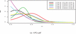
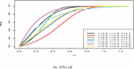
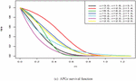
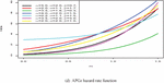
Figure 1 shows the pdf, cdf, survival, and hazard rate functions respectively of the APGz model. Figure 1 indicates that the APGz distribution is unimodal, left skewed, increasing, decreasing and bathtub shaped.

The R codes for generating the various functions are provided in Appendix A.

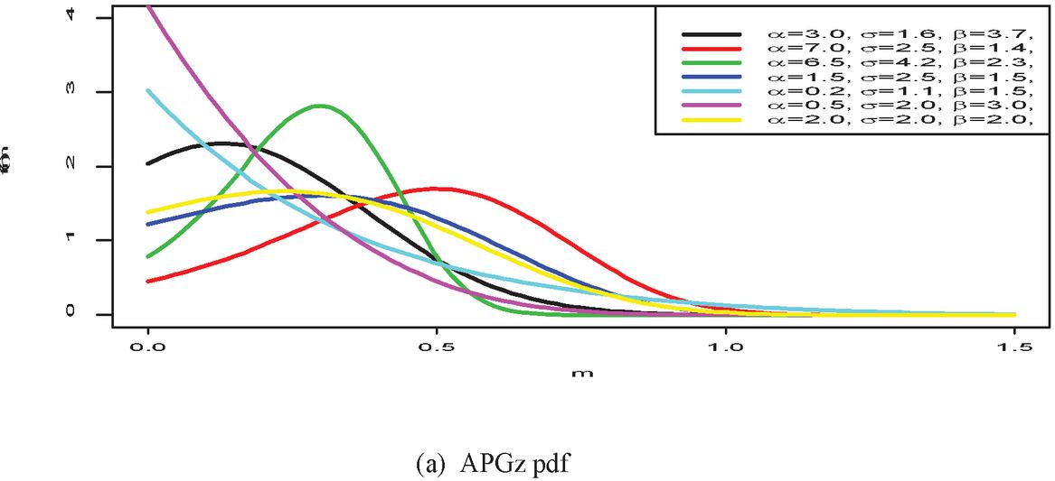
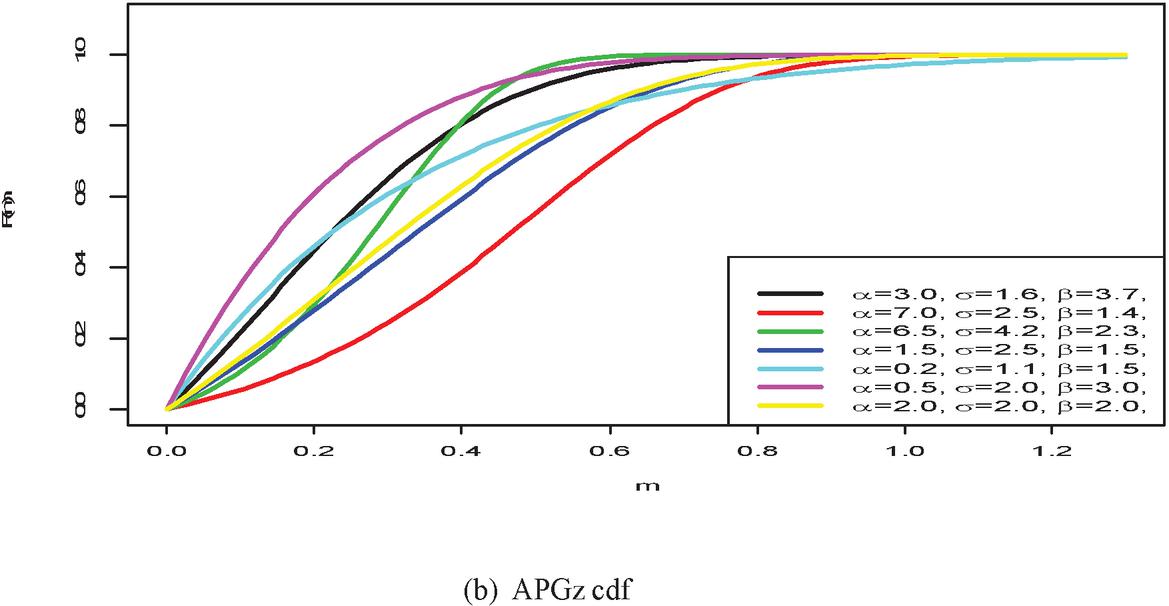
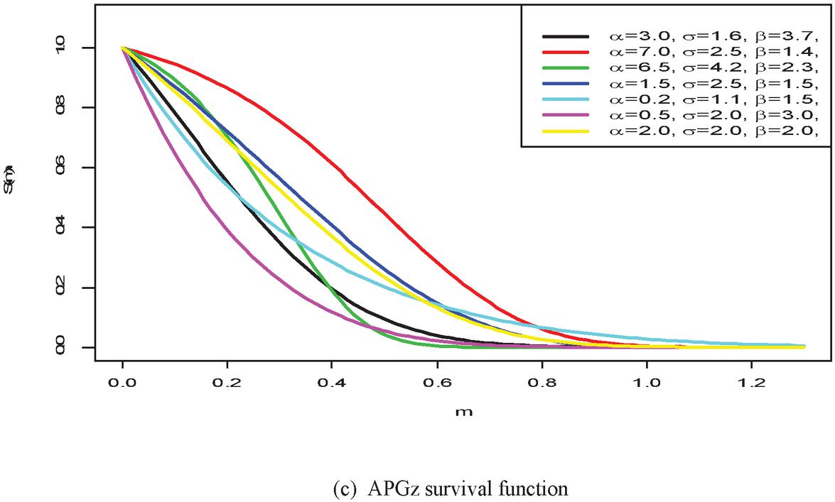
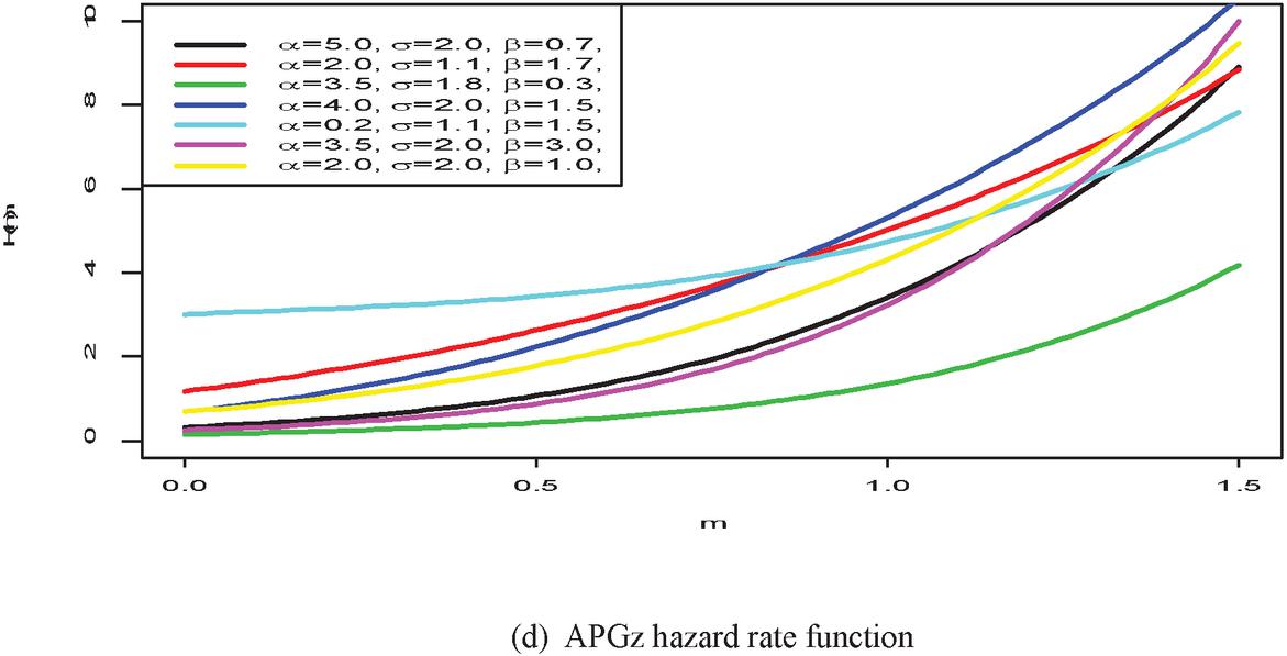
Figure 1 The pdf, cdf, survival and hazard rate plots of the APG model.

3 The Regression Analysis

Parametric models are often used to estimate the survival function of univariate distributions. These parametric models that provide good fit provide precise estimates for quantities of interest.

Let $M$ be APGz random variable with pdf in Equation (1). Then, a regression model for location parameter for random variable $X=\log (M)$ is log APGz (LOAPGz) distributed. Then,

$X=\eta (\phi )+Z$, $Z$ is not in $\phi$ and $Z$ is the residual term.

More so, the cdf and pdf of the $X$ for a support $x$ is expressed in alpha power transformation as

$$F(x-\phi )=\frac{\alpha {}^{G(x-\eta )}-1}{(\alpha -1)}\mathit{\hspace{1em}}\alpha \in ({\mathrm{\Re }}^{+}-\{1\}),$$

(5)

and

$$f(x-\eta )=\frac{\log \alpha }{(\alpha -1)}g(x-\phi )\alpha {}^{G(x-\phi )}\mathit{\hspace{1em}}\alpha \in (\mathrm{\Re }{}^{+}-\{1\}).$$

(6)

3.1 The Log APGz Model

Let $M$ be APGz distributed and $X=\log (M)$ the log APGz distribution. Then, the density function of $X(x\in \mathrm{\Re })$ can be expressed as

$f(x)$	$={\displaystyle \sum _{j=0}^i}{\displaystyle \sum _{i=0}^{\mathrm{\infty }}}{(-1)}^j\sigma {\displaystyle \frac{1}{j!(i-j)!}}{\displaystyle \frac{{(\log \alpha )}^{1+i}}{(\alpha -1)}}$
	$\mathrm{\hspace{1em}}\cdot e^{\frac{\sigma }{\beta }(1-e{}^{\beta \exp (x-\phi )})(1+j)+\beta \exp (x-\phi )},$	(7)

where $\phi \in \mathrm{\Re }$ is the location parameter. However, for a linear location regression model with response variable $X_i$ and explanatory variable vector ${\phi }_i$, we have

$$X_i={\eta }_i^T\lambda +Z_i\mathit{\hspace{1em}}i=1,2,3,4,5,\mathrm{\dots }n.$$

(8)

The standardized density function of Equation (7) is expressed as

$$q(x)=\sum _{j=0}^i\sum _{i=0}^{\mathrm{\infty }}{(-1)}^j\sigma \frac{1}{j!(i-j)!}\frac{{(\log \alpha )}^{1+i}}{(\alpha -1)}{e}^{\frac{\sigma }{\beta }(1-e{}^{\beta \exp (z)})(1+j)+\beta \exp (z)}.$$

(9)

4 The Prior Distribution

In Bayesian analysis, the prior is specified irrespective of the parameter of interest before using the pdf to analyze the experimental data.

Several priors like the Gaussian and the Uniform distributions have been used in literature. However, the uniform prior has been very useful in Bayesian analysis because it assumes that the value of the parameters for the prior is equally likely and is impossible for a particular threshold. Thus, the Half-Cauchy distribution with upper tail with a large mass that approaches zero for large values is preferred because, it exhibit the characteristics of the uniform distribution for a scale parameter of 25.

However, the pdf of the Half-Cauchy is expressed as

$$h(m)=\frac{2\psi }{\mathrm{\Pi }(m^2+{\psi }^2)}\mathit{\hspace{1em}}m>0,\psi >0,$$

(10)

with $\psi$ as the scale parameter. It is important to note that, the variance and mean of the Half-Cauchy model do not exist. However, the Half-Cauchy has a mode of zero. Now, for a scale parameter of 25, the pdf of the Half-Cauchy is almost flat (see Figure 2). Hence, this gives the Half-Cauchy a better edge as a prior to provide enough information that can be used to evaluate the algorithm numerically that can explore the required target posterior density. Thus, the Half-Cauchy distribution with a scale parameter of 25 is used as a prior in this study. (see [2, 14–16]).

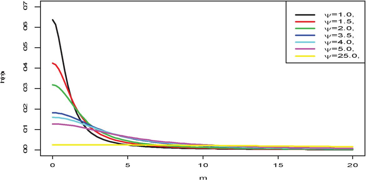
Figure 2 Half-Cauchy pdf for different parameter values.

5 Bayesian Reliability Analysis of the APGz Model

The Bayesian reliability analysis can be obtained using the pdf given in Equation (1) and the corresponding survival function Equation (3), the likelihood function can be expressed as

$$L=\prod _{\upsilon =1}^{\rho }{[h(y_{\upsilon })]}^{{\delta }_{\upsilon }}{[S(y_{\upsilon })]}^{1-{\delta }_{\upsilon }}$$

Such that for ${\delta }_{\upsilon }=0$ for censored and ${\delta }_{\upsilon }=1$ for uncensored. Hence,

$L$	$={\displaystyle \prod _{\upsilon =1}^{\rho }}{\left[{\displaystyle \frac{\log \alpha }{(\alpha -1)}}\sigma e^{(\beta y+\frac{\sigma }{\beta }(1-e^{\beta y}))}{\alpha }^{(1-e{}^{(\frac{\sigma }{\beta }(1-e^{y\beta }))})}\right]}^{{\delta }_{\upsilon }}$
	$\mathrm{\hspace{1em}}\times {\left[1-{(\alpha -1)}^{-1}({\alpha }^{(1-e{}^{(\frac{\sigma }{\beta }(1-e{}^{\beta y}))})}-1)\right]}^{1-{\delta }_{\upsilon }}.$	(11)

However, the joint posterior density can be expressed as

$p(\alpha ,\lambda ,\sigma |y,M)$	$\propto L(y,M|\alpha ,\lambda ,\sigma )\times p(\alpha )\times p(\sigma )$
	$\propto {\displaystyle \prod _{\upsilon =1}^{\rho }}{\left[{\displaystyle \frac{\log \alpha }{(\alpha -1)}}\sigma e^{(\beta y+\frac{\sigma }{\beta }(1-e^{\beta y}))}{\alpha }^{(1-e{}^{(\frac{\sigma }{\beta }(1-e^{y\beta }))})}\right]}^{{\delta }_{\upsilon }}$
	$\mathrm{\hspace{1em}}\times \left[1-{(\alpha -1)}^{-1}({\alpha }^{(1-e{}^{(\frac{\sigma }{\beta }(1-e{}^{\beta y}))})}-1)\right]$
	$\times {\displaystyle \prod _d^D}{\displaystyle \frac{1}{\sqrt{2000\mathrm{\Pi }}}}{e}^{-\frac{{\lambda }_d^2}{2000}}\times {\displaystyle \frac{50}{\mathrm{\Pi }({\alpha }^2+625)}}\times {\displaystyle \frac{50}{\mathrm{\Pi }({\sigma }^2+625)}},$	(12)

where

$$\alpha \sim HC(0,25),\sigma \sim HC(0,25)\mathit{and}{\lambda }_d\sim N(0,{10}^3),$$

$$d=1,2,3,4,5,\mathrm{\dots },D,\mathit{\text{with HC}}=\mathit{\text{Half-Cauchy}}.$$

The closed form of Equation (14) does not exist. Thus, the marginal (the basis of the Bayesian inference) posterior densities of the parameter cannot be obtained in a closed form. Hence, MCMC methods are used to evaluate the posterior parameters. The posterior parameters can be evaluated using the rstan package in R to fit the Bayesian contest.

6 The Stan Implementations

The Bayesian analysis of the APGz model using the rstan package is carried out following the log survival, log hazard rate functions and defining the sampling models for the right censored data steps. However, the distribution at the stage is built on the function definition blocks, data block and parameter block; which allows the variable used in the model to be defined in terms of the data and parameters used. rstan Code for the implementation is shown in Appendix B.

7 Data Creation and Implementation

This section presents the dataset used for the analysis and how the data are coded in the Stan package. The value of the Rhat is used to investigate the applicability and flexibility of the Bayesian model. The closer the Rhat is to 1, the better the model.

The data represent the number of women breast cancer cases in the Western World Hospital as used in [15] and [1]. Censored survival times are indicated as an asterisk. The data are represented as follows:

Negatively stained: 23, 47, 69, 70*, 71*, 100*, 101*, 148, 181, 198*, 208*, 212*, 224*

Positively stained: 5, 8, 10, 13, 18, 24, 26, 26, 31, 35, 40, 41, 48, 50, 59, 61, 68, 71, 76*, 105*, 107*, 109*, 113, 116*, 118, 143*, 154*, 162*, 188*, 212*, 217*, 225*

In this regard, Censored is denoted with 0 and uncensored is recorded as 1. The data are recorded as data in matrix form. The summary results for the performance rating are shown in Table 1. In Table 1, the following abbreviations where used; posterior mean is denoted as mean, se-mean is the Monte Carlo standard errors, posterior standard deviation is denoted as std, numbers of effective sample size denoted as NE and spits is denoted as (Rhat).

Table 1 Performance results with rstan function for APGz model (approximate) values

	Std	Mean	Se-mean	97.5%	75%	50%	25%	2.5%	Rhat	NE
dev	2.03	312.40	0.03	320.27	317.59	310.56	310.27	309.49	1.09	2157
Beta[1]	0.50	-1.31	0.01	-0.05	-0.58	-1.00	-1.14	-2.11	1.05	1997
Beta[0]	1.51	6.51	0.09	11.49	9.13	7.61	4.76	1.54	1.00	1094
lp_	1.51	-155.24	0.04	-119.51	-120.71	-121.28	-122.42	-139.55	1.03	1203
shape	419.51	19.10	5.82	56.25	5.49	0.68	0.25	0.15	1.00	2267
scale	6.17	0.61	0.11	7.16	0.87	0.21	0.12	0.01	1.00	2217

Table 1 shows the Stan results for individual and merged chains. The posterior Bayesian estimate of ${\beta }_0$ is $6.51\pm 1.51$ with percentage confidence of 1.54, 11.49 with Rhat 1.00. This implies that it is significant. Also, The posterior Bayesian estimate of ${\beta }_1$ is $-1.31\pm 0.51$ with percentage confidence of $(-2.11,-0.05)$ with Rhat 1.05. This implies that it is significant since the Rhat is close to 1.

Conclusion

This article has introduced the APGz Bayesian reliability analysis that extends the usual conventional classical statistical properties of the APGz distribution in [9]. The APGz regression analysis was also derived in this study to further enhanced its applicability. The rstan package for the implementation of the Bayesian analysis was explicitly derived and investigated. The proposed model was also applied to real-life data to examine the model flexibility. The results show that the Bayesian approach is flexible, applicable and tractable in censored data.

Appendix A

Function for APGz Distribution in R

In this subsection, the R codes for generating the various functions are provided. The following variables where used $a=\mathit{alpha},b=\mathit{beta}$ and $L=\mathit{sigma}$.

1 R code for APGz pdf

APGz-pdf$<$-function(x,a,L,b){

((log(a))/(a – 1))*L*exp(b*x – (L/b)*(exp(b*x) – 1))*a${}^{\wedge }$(1 – exp (–(L/b)*(exp(b*x) – 1)))

}

2 R code for APGz cdf

APGz-cdf $<$-function(x,a,L,b){

((a${}^{\wedge }$(1 – exp(-(L/b)*(exp(b*x) – 1))) – 1)/(a – 1))}

3 R code for generating APGz random numbers

APGz-r $<$-function(u,a,L,b){

(b${}^{\wedge }$-1)*log(1 – (b/L)*log(1 – (((log (a))${}^{\wedge }$(-1))*log(u*(a – 1) + 1))))}

4 R code for APGz survival function

APGz-S $<$-function(x,a,L,b){

1- (((a${}^{\wedge }$(1 – exp(-(L/b)*(exp(b*x) – 1))) – 1)/(a – 1)))}

5 R code for APGz hazard rate function

APGz-H $<$-function(x,a,L,b){

(L*exp(b*x – (L/b)*(exp(b*x) – 1)))*((a${}^{\wedge }$(1 – exp(-(L/b)*(exp(b*x) – 1)) -1))/(1 – a${}^{\wedge }$(1 – exp(-(L/b)*(exp(b*x) – 1)) – 1))) *log(a)}

Appendix B

stan(file, model_name = “anon_model”, model_code = “”,fit = NA, data = list(), pars = NA, chains = 4, iter = 2000, warmup = floor(iter/2), thin = 1, init = “random”,algorithm = c(“NUTS”, “HMC”, “Fixed_param”),)

library(rstan)

APGz=”

functions{

//defined survival

vector log_s(vector t, real shape, real scale,

vector rate){

vector[num_elements(t)] log_s;

for(i in 1:num_elements(t)){log_s[i]=log(1- ((((rate[i])${}^{\wedge }$(1 – exp(-(shape/

scale)*(exp(shape*t[i]) – 1))) – 1)/(rate[i] – 1)))}

);

//define log_ft

vector log_ft(vector t, real shape,real scale,

vector rate){

vector[num_elements(t)] log_ft;

for(i in 1:num_elements(t)){

log_ft[i]= log(((log(rate[i]))/(rate[i] – 1))*shape*exp(scale*t[i] –

(shape/scale)*(exp(scale*t[i]) – 1))*a${}^{\wedge }$(1 – exp(-(shape/scale)*

(exp(scale*t[i]) – 1))))

return log_ft;}

//define log hazard

vector log_h(vector t, real shape,real scale, vector

rate){

vector[num_elements(t)] log_h;

vector[num_elements(t)] logft;

vector[num_elements(t)] logs;

logft=log_ft(t,shape,scale,rate);

logs=log_s(t,shape,scale,rate);

log_h=logft-logs;

return log_h;

}

//define the sampling distribution

real surv_APGz_lpdf(vector t, vector d,

real shape,real scale, vector rate){

vector[num_elements(t)] log_lik;

real prob;

log_lik=d .* log_h(t,shape,scale,rate)+log_s

(t,shape,scale,rate);

prob=sum(log_lik);

return prob;

}}

//data block

data {

int N; // number of observations

vector$<$lower=0$>$[N] y; // observed times

vector$<$lower=0,upper=1$>$[N] censor;//censoring indicator

(1=observed, 0=censored)

int M; // number of covariates

matrix[N, M] x; // matrix of covariates (with n rows and

H columns)}

parameters {

vector[M] beta; // Coefficients in the linear predictor

(including intercept)

real$<$lower=0$>$ shape; // shape parameter

real$<$lower=0$>$ scale;}

transformed parameters {

vector[N] linpred;

vector[N] rate;

linpred = x*beta;

for (i in 1:N) {

rate[i] = exp(linpred[i]);

}}

model {

shape $\sim$cauchy(0,25);

scale $\sim$cauchy(0,25);

beta $\sim$normal(0,1000);

y $\sim$surv_APGz(censor, shape, scale, rate);

}

generated quantities{

real dev;

dev=0;

dev=dev + (-2)*surv_APGz_lpdf(y|censor,

shape,scale,rate);

}

#regression coefficient with log(y) as a guess to

initialize

beta1=solve(crossprod(x),crossprod(x,log(y)))

#convert matrix to a vector

beta1=c(beta1)

S1$<$-stan(model_code=model_code1,init=list

(list(beta=beta1),list(beta=2*beta1)),

data=dat,iter=5000,chains=2)

print(S1,c(“beta”,“shape”,“dev”),digits=2)

”

stan_ac(S1,“beta”)

Appendix C

y$<$c(23,47,69,70,71,100,101,148,181,198,208,212,224,5,8,10,13,18,24,26,

26,31,35,40,41,48,50,59,61,68,71, 76,105,107,109,113,116,118,143,154,

162,188,212,217,225)

x1$<$-c(rep(0,13), rep(1,32))

censor$<$-c(rep(1,3),rep(0,4),rep(1,2),rep(0,4),rep(1,18),

rep(0,4),1,0,1,1,rep(0,6))

x $<$- cbind(1,x1)

N = nrow(x)

M = ncol(x)

event=censor

dat $<$- list( y=y, x=x, event=event, N=N, M=M)

References

[1] AbuJarad, M. H., Khan, A. A., Khaleel, M. A., AbuJarad, E. S. A., AbuJarad, A. H. and Oguntunde, P. E. Bayesian Reliability Analysis of Marshall and Olkin Model. Annals of Data Science, 2019. doi.org/10.1007/s40745-019-00234-3.

[2] AbuJarad, M. H, AbuJarad, E. S. A., and Khan, A. A. Bayesian survival analysis of type I general exponential distributions. Annals of Data Science, 2019. doi.org/10.1007/s40745-019-00228-1.

[3] AbuJarad, M. H. and Khan, A. A. Exponential model: A Bayesian study with Stan. International Journal of Recent Scientific Research 9(8):28495–28506, 2018.

[4] AbuJarad M. H, Khan A. A. Bayesian survival analysis of Topp–Leone generalized family with Stan. Int J Stat Appl 8(5):274–290, 2018a.

[5] Akhtar, M. T., and Khan, A. A. Bayesian analysis of generalized log-Burr family with R. Spinger Plus, 3, 185, 2014. doi: 10.1186/2193-1801-3-185.

[6] Akhtar, M. T. and Khan, A. A. Bayesian reliability analysis of binomial model – Application to success/failure data. Journal of Modern Applied Statistical Methods, 17(2), 2018. eP2623. doi: 10.22237/jmasm/1553803862.

[7] Arora, S. Mahajan, K. K. and Kumari, R. Bayes estimators for the reliability and hazard rate functions of Topp-Leone distribution using Type-II censored data. Communications in Statistics – Simulation and Computation, 2019. doi: 10.1080/03610918.2019.1602646.

[8] Carlin, B. P., and Louis, T. A. Bayesian methods for data analysis. CRC Press, Boca Raton, 2008.

[9] Eghwerido, J. T., Nzei, L. C. and Agu, F. I. The Alpha Power Gompertz Distribution:Characterization, Properties, and Applications. Sankhya A: The Indian Journal of Statistics, 2020. doi.org/10.1007/s13171-020-00198-0.

[10] El-Sayed, M. A., Abd-Elmougod, G. A. and Abdel-Rahman, E. O. Estimation for coefficient of variation of Topp-Leone distribution under adaptive Type-II progressive censoring scheme: Bayesian and non-Bayesian approaches. Journal of Computational and Theoretical Nanoscience 12(11):4028–35, 2015. doi: 10.1166/jctn.2015.4314.

[11] Gelman, A. Prior Distributions for Variance Parameters in Hierarchical Models. Bayesian analysis, 1(3), 515–534, 2006.

[12] Ismail, A. A. Bayes estimation of Gompertz distribution parameters and acceleration factor under partially accelerated life tests with type-I censoring, Journal of Statistical Computation and Simulation, 80:11, 1253–1264, 2010. doi: 10.1080/00949650903045058.

[13] Kamar, S. H. Bayesian procedure modified by Fourier series residual to fitting the logistic growth model. Pakistan Journal of Statistics, 35(4), 301–313, 2019.

[14] Khan, N., Akhtar, M. T. and Khan, A. A. Bayesian Analysis of Marshall-Olkin family of distributions, International Journal Recent Scientific Research, 8(7), 18692–18699, 2017.

[15] Khan, N. and Khan, A. A. Bayesian Analysis of Topp-Leone Generalized Exponential Distribution. Austrian Journal of Statistics, 47, 1–15, 2018. doi: 10.17713/ajs.v47i4.716.

[16] Khan, N., Akhtar, M. T., and Khan, A. A. A Bayesian approach to survival analysis of inverse Gaussian model with Laplace approximation. International Journal of Statistics and Applications, 6(6): 391–398. 2016. doi: 10.5923/j.statistics.20160606.08.

[17] Singh, S. K., Singh, U. and Kumar, D. Bayes estimators of the reliability function and parameter of inverted exponential distribution using informative and non-informative priors, Journal of Statistical Computation and Simulation, 83(12):2258–69. 2013. doi: 10.1080/00949655.2012.690156.

[18] Sniekers, S. and van der Vaart, A. Adaptive Bayesian credible bands in regression with a Gaussian process prior, Sankhya A: The Indian Journal of Statistics, 2019. doi.org/10.1007/s13171-019-001850.

[19] Turnbull, B. C. and Ghosh, S. K. Unimodal density estimation using Bernstein polynomials, Computational Statistics and Data Analysis, 72, 13–29, 2014.

[20] Yousuf, F. and Khan, A. A. Bayesian Analysis of Normal Model with Stan and Inla. Journal of Emerging Technologies and Innovative Research, 6(6), 406–416, 2019.

Biographies

Joseph Thomas Eghwerido received his B.Sc. and M.Sc. in Statistics from the Obafemi Awolowo University Ile-Ife in years 2008 and 2013 respectively. He then proceeded to the University of Benin Edo State, Nigeria where he obtained his Ph.D. in Industrial Mathematics with Options in Statistics in 2019. He is the Pioneer and current Head of the Department of Statistics, Federal University of Petroleum Resources, Effurun, Delta State, Nigeria. He has several publications in Spatial Statistics, Data Science, Portfolio Management, Probability Theory, and Distribution Theory. He is a member of the Editorial Team of Mathematical Reviews (MathSciNet), Mathematica Slovaca, Scientific African, Thailand Statistician, Fupre Journal of Scientific and Industrial Research, Gazi University Journal of Science, Scientometrics, Austrian Journal of Statistics, and lots more. He is a member of the Nigerian Statistical Association, Nigerian Mathematical Society, and International Biometric Society.

Suraju Olaniyi Ogundele received his B.Sc. and M.Sc. in Statistics from the Federal University of Agriculture Abeokuta in years 2002 and the University of Ibadan in 2007 respectively. He then proceeded to the University of Benin Edo State, Nigeria where he obtained his Ph.D. in Industrial Mathematics with Options in Statistics in 2019. He is a lecturer at the Department of Statistics, Federal University of Petroleum Resources, Effurun, Delta State, Nigeria. He has several publications in Computational Statistics and Robust Statistical Modelling. He is a member of the Nigerian Statistical Association.

Lawrence Chukwudumebi Nzei had his B.Sc. Industrial Mathematics from Delta State University, Abraka, Nigeria in 2008 and proceeded to the University of Benin, Benin City where he obtained an M.Sc. Industrial Mathematics (with an option in Statistics) in the year 2015. Currently, Lawrence C. Nzei is a Ph.D. Statistics student in the Department of Statistics, University of Benin, Benin City, Nigeria. He is a Mathematics tutor at the University of Benin Foundation Program. He has several publications in Probability Distribution Theory, Survival analysis and Bayesian analysis. He is also a Reviewer of Thailand Statistician, Pakinstan Journal of Statistics and Operation Research, Gazi University Journal of Science, and lots more. He is a member of the Nigerian Statistical Association, Nigerian Mathematical Society, and International Biometric Society.

Friday Ikechukwu Agu is a Statistician, Researcher, Data Analyst, Academic Adviser, and Lecturer at the Department of Statistics, University of Calabar, Nigeria. He obtained a Bachelor of Science in Mathematics and Statistics from Ebonyi State University, Abakaliki, Nigeria, and a Master of Science in Statistics from the University of Calabar, Calabar, Nigeria. Both programs were completed with research components. Currently, he is a Ph.D. student in statistics. Friday’s research interests include Distribution Theory, Aggregate Claim Modeling in Insurance, Copula, and Financial Tail Dependence. He has published several research articles in high reputable journals. In addition, he is also a reviewer/editor for several academic journals. Friday is a member of the Nigerian Statistical Association and the professional statistician society of Nigeria.

Journal of Reliability and Statistical Studies, Vol. 15, Issue 2 (2022), 617–634.
doi: 10.13052/jrss0974-8024.1529
© 2022 River Publishers

Abstract

1 Introduction

2 The Alpha Power Gompertz Model (APGz)

3 The Regression Analysis

3.1 The Log APGz Model

4 The Prior Distribution

5 Bayesian Reliability Analysis of the APGz Model

6 The Stan Implementations

7 Data Creation and Implementation

Conclusion

Appendix A

Function for APGz Distribution in R

Appendix B

Appendix C

References

Biographies