Uncovering Regional Disparities in Infrastructural Development of Uttar Pradesh: An Exploratory Factor Analysis
Madhulika Dube, Subhash Kr. Yadav* and Vishwajeet Singh
Department of Statistics, Babasaheb Bhimrao Ambedkar University,
Lucknow, India
E-mail: drskystats@gmail.com
Corresponding Author
Received 17 May 2021; Accepted 17 December 2021; Publication 28 January 2022
Abstract
In developmental studies, the infrastructural sector is considered as an important component of overall economic development. The infrastructural growth in the state of Uttar Pradesh is undoubtedly critical since independence. The main focus of this paper is to uncover the principal factors or dimensions of infrastructural characteristics and to quantify the level of infrastructural development of Uttar Pradesh into five clusters having different grade of development using Exploratory Factor Analysis & K-means Cluster Analysis. The analysis has been carried out by taking into account various infrastructural indicators for the time period of two years from 2018 to 2019. The results of the present analysis led to the identification of the five factors of infrastructural characteristics, and the classification of all the seventy-five districts of Uttar Pradesh into five regions with different degree of infrastructural development. The ‘infrastructural regions’ uncovered through this procedure allow a much more useful characterization of Uttar Pradesh for the policy making purpose. The same technique may be applied to the whole country and other countries as well.
Keywords: Regional infrastructural disparities, exploratory factor analysis (EFA), K-means cluster analysis, Uttar Pradesh.
1 Introduction
In the last quarter of twentieth century, Uttar Pradesh was attributed as agricultural powerhouse of India but in past two decades, the gradual transference towards a service-oriented economy has originated the problem of regional disparity in infrastructural sector of the state. Since Uttar Pradesh is one of the densely populated state of India, regional disparities emerged as the outcome of lopsided infrastructural development influenced by the uneven regional allocation of economic wealth, subsidies, population and natural sources (Dube et al., 2020a). Regional disparities are a worrying issue in India, and they are continuously rising despite the government’s varied policy measures to develop backward areas. Policymakers and economists have faced significant challenges as a result of disparities in social and economic growth, employment, and infrastructure facilities across and within regions (Jose, 2019). Regional disparities in infrastructural sector generally reflects the variations in infrastructural facilities among the districts of the state, which involves an adequate set of socio-economic, demographic, historical & environmental factors (Dube et al., 2020b). Regional disparities are mostly the result of globalization and changes in the sectoral composition of economies (Carvers and Mayhew, 2021). The presence of multiple and complex relationship between infrastructural growth and economic development affects the process of production and consumption directly and also generates lot of dependent and independent extraneous factors which may cause larger flow of expenditure there by creating more employment opportunities (Ghosh and De, 2005). The 11th Finance Commission report of India suggested that, “The use of infrastructural index as one of the yardsticks for transmission has also been put forwarded by various states. In our opinion, the accessibility of better infrastructural services plays a pivotal character in fascinating investments, and states with the lower values of infrastructural index need to be supported in order to raise their level of infrastructural development (11th Finance Commission report, Government of India, 2000, p. 58).
The sharp intra-regional disparities in agricultural infrastructure are the major source of variation in agricultural productivity among the different regions in Uttar Pradesh (Kumar and Joshi, 2018). In order to intensify the economic growth in less developed states of India, there should be substantial emphasis on infrastructural sector (Sahoo and Dash, 2009). Spending more on infrastructural facilities like, transport, agricultural infrastructure, power supply, educational institutions, healthcare facilities will show a strong influence on rural productivity and poverty degradation in Uttar Pradesh (Kozel and Parker, 2003). According to the foundational economy approach to balanced economic development, policymakers should prioritize the quantification and removal of regional disparities in various areas of the economy (Hansen, 2021). Therefore, the scientists and policy makers are trying to measure the different levels of infrastructural development in Uttar Pradesh. A single indicator may not be sufficient to gauge the level of development of any region or a country. Using different statistical techniques, researchers have directed their efforts towards working out disparities in Infrastructural, Socio-economic and Agricultural development in various regions of India as well as in other different countries over the years (see; e.g., Yang and Hu, 2008; Zali et al., 2013; Ohlan, 2013; Dube et al., 2014; Mittal and Devi, 2015; Salvati et al., 2017; Hryhoruk et al., 2019; Dube et al., 2020a, b; Hooda and Nain, 2021, among others and references cited therein).
From the past two decades, a large number of studies have addressed the problem of regional disparities but no one dealt specifically with the regional disparities in infrastructural development of Uttar Pradesh. There is no literature available in reference to the quantification of latent factors (infrastructural dimensions) responsible for the infrastructural growth of Uttar Pradesh. No such literature has also been found in the context of Uttar Pradesh which can classify all the seventy-five districts of the state into different clusters according to their similar infrastructural characteristics using robust statistical methodology. Thus, realizing the importance and solemnity of the problem of regional infrastructural disparities in Uttar Pradesh, the present article deals with the two important objectives: first, to identify a smaller number of infrastructural dimensions or constructs which sufficiently summarizes the statistics captured by various indicator variables which are responsible for sustainable infrastructural development in Uttar Pradesh; second, to look for the homogeneous grouping of all the seventy-five districts of Uttar Pradesh into few clusters in terms of different levels of infrastructural development using the multivariate statistical methods namely, Exploratory Factor Analysis (EFA) and K-means Cluster Analysis.
2 Data: Selection of Indicators for Infrastructural Sector
The study is based on twenty-one indicator variables of infrastructural sector that have been obtained from ‘District Wise Development Indicators Uttar Pradesh 2019’ published annually by the Economics and Statistics Division, State Planning Institute, Planning Department (UPDES), Government of Uttar Pradesh. The data on the following infrastructural development indicators have been taken into account:
1. No. of hospitals/dispensaries per lakh of population.
2. No of beds in hospitals per lakh of population.
3. No. of Veterinary hospitals per lakh of population.
4. No. of Higher Senior schools per lakh of population.
5. No. of Polytechnic’s per lakh of population.
6. No. of villages with distance 5 km. or more from Railway Stations/ Halts.
7. No. of villages with distance 5 km. or more from Bus Stations/ Stops.
8. Total length of Pucca roads per thousand square Km.
9. Per capita electricity consumption (KWH.).
10. Percentage of electricity consumption in industry to total consumption.
11. No. of L.P.G. consumers per lakh of population.
12. No. of post offices per lakh of population.
13. AI centers/sub-centers per lakh of population.
14. Livestock development centers per lakh of population.
15. No. of villages with distance 5 km. or more from Industrial/Grameen/Co-operative banks.
16. No. of villages with distance 5 km. or more from Co-operative Milk collection centers.
17. No. of industrial areas per lakh of population.
18. No. of small-scale industries per lakh of population.
19. No. of registered working factories per lakh of population.
20. No. of Scheduled commercial banks per lakh of population.
21. No. of primary agricultural credit societies per lakh of rural Population.
3 Identification of the Inherent Infrastructural Dimensions
To identify infrastructural dimensions ‘Exploratory Factor analysis (EFA)’ has been used to extract fewer numbers of infrastructural dimensions that sufficiently summarize the statistics hidden in the original set of indicators. The Exploratory Factor Analysis (EFA) using PCA is a multivariate method used to investigate the constructs or dimensions assumed to underlie a set of inter dependent variables. The factors obtained through exploratory factor analysis are linearly related set of original variables which are highly correlated with each other.
3.1 Analyzing the Adequacy of EFA
Analyzing the adequacy of EFA means evaluating either the set of indicators used in the analysis are significant and sufficiently interrelated with each other so that their dimensions can be reduced into fewer number of factors or components by using the CFA model. In the present study both the KMO index, with a measure 0.764, and the Bartlett test of sphericity, with a value 1048.454 with p-value 0.000 (0.05) suggested that Confirmatory Factor analysis can be proceeded (see; Field 2009, Pallant 2010).
3.2 Multiple Criteria for Determining the Number of Factors to be Extracted
In order to determining the number of factors to be extracted, four criteria have been used:
(1) Eigen value criterion
(2) Scree plot criterion
(3) Percentage of variance criterion
(4) Interpretability of the factor structure solution.
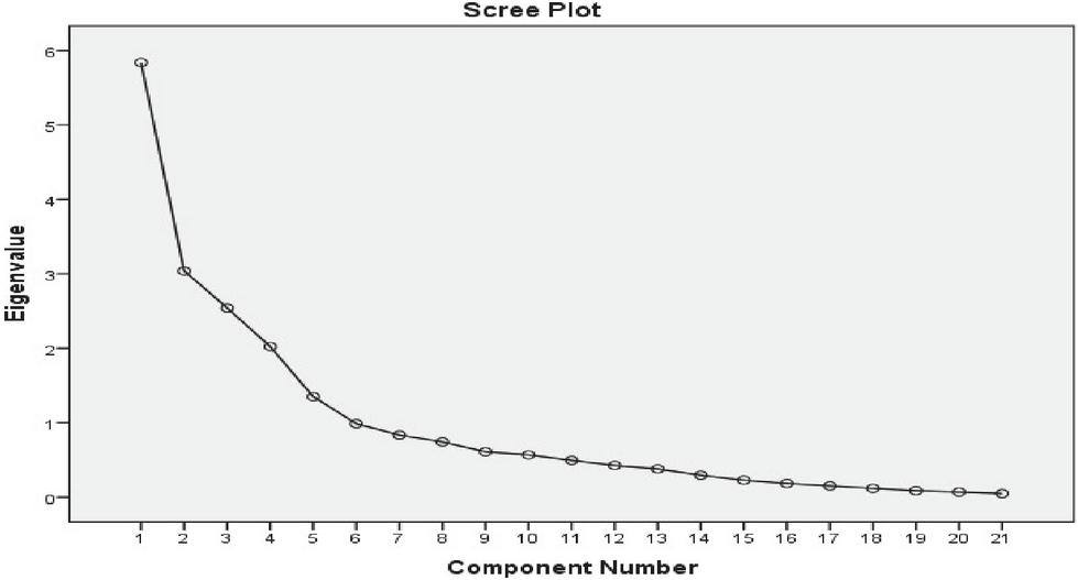
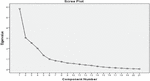
Figure 1 Scree Plot for EFA.
Table 1 Eigen values and percentage of variance explained
| Initial Eigen Values | |||
| Number of Components | Eigen Values | Percentage of Variance | Cumulative % of Var. |
| 1 | 5.837 | 27.795 | 27.795 |
| 2 | 3.040 | 14.478 | 42.273 |
| 3 | 2.540 | 12.094 | 54.367 |
| 4 | 2.023 | 9.633 | 64.000 |
| 5 | 1.347 | 6.416 | 70.416 |
| 6 | 0.985 | 4.693 | 75.109 |
| 7 | 0.833 | 3.968 | 79.076 |
| 8 | 0.741 | 3.527 | 82.604 |
| 9 | 0.609 | 2.900 | 85.504 |
| 10 | 0.568 | 2.703 | 88.207 |
| 11 | 0.494 | 2.351 | 90.557 |
| 12 | 0.425 | 2.026 | 92.583 |
| 13 | 0.379 | 1.803 | 94.386 |
| 14 | 0.294 | 1.402 | 95.788 |
| 15 | 0.228 | 1.084 | 96.872 |
| 16 | 0.183 | 0.873 | 97.745 |
| 17 | 0.151 | 0.718 | 98.463 |
| 18 | 0.119 | 0.565 | 99.027 |
| 19 | 0.086 | 0.410 | 99.437 |
| 20 | 0.070 | 0.331 | 99.768 |
| 21 | 0.049 | 0.232 | 100.000 |
Following Hair et al. (2010), five factors having eigen values larger than one has been retained which is also in agreement with the scree plot (Figure 1). The percentage of variance criterion, postulates that more than 60% of the total variance of the original set of variables can be used to decide the number of factors to be extracted (see; Hair et al. 2010). In view of this, Table1 is suggestive of extracting minimum four factors. Last but not the least, the ability of interpretative ability and an eloquent assignment to the extracted factors, is yet another enormously important criterion in reaching a decision about the final number of factors to be extracted (Hair et al., 2010).
We notice that in our study five factors, which accounted for 70.416% of the total variance of the original set of variables, were sufficient to be retained to reveal and highlight the results of the exploratory factor analysis model. Lastly, Varimax orthogonal rotation with Kaiser Normalization has been used to provide more reasonable factor model.
Table 2 Rotated component matrix table for factor loadings
| Rotated Component Matrix | |||||
| Component | |||||
| Indicator Variables | 1 | 2 | 3 | 4 | 5 |
| Scheduled comm. banks | 0.903 | – | – | – | – |
| LPG consumers | 0.884 | – | – | – | – |
| Per capita electricity cons. | 0.862 | 0.306 | – | – | – |
| Registered working factories | 0.842 | – | – | – | – |
| Small scale industries | 0.721 | – | – | – | – |
| No. of industrial areas | 0.611 | – | – | – | 0.477 |
| % of electricity cons in ind. | 0.588 | – | – | – | 0.358 |
| Railway Stations/Halts | – | 0.932 | – | – | – |
| Bus Stations | – | 0.924 | – | – | – |
| Ind./Grameen/Co-op. banks | – | 0.886 | – | – | – |
| Co-op. milk collection centre | – | 0.867 | – | – | – |
| No. of polytechnics | – | 0.332 | – | 0.300 | – |
| Livestock development centre | – | – | 0.889 | – | – |
| Veterinary hospitals | – | – | 0.842 | – | – |
| AI centres/sub-centres | – | – | 0.741 | – | – |
| No. of beds in hospitals | – | – | – | 0.786 | – |
| No. of hospitals/dispensaries | 0.374 | – | – | 0.651 | 0.364 |
| Higher secondary schools | – | – | – | 0.596 | – |
| No. of post offices | – | – | – | 0.412 | 0.768 |
| Length of pucca roads | 0.430 | – | – | – | 0.582 |
| Primary agricultural societies | – | .371 | – | – | 0.577 |
| Method of Extraction: P C A. Method of Rotation: Varimax rotation with Kaiser Normalization. | |||||
| a. Rotation converged in 6 iterations. | |||||
3.3 Interpretation and Naming the Factors
In an ideal component matrix, factor loadings larger than 0.30 are recognized as significant; and loadings larger than 0.50 are recognized as highly significant (see; Soares et al. (2003)). From Table 2, it is clear that in the present analysis factor loading greater than 0.30 are used to determine the infrastructural dimensions of Uttar Pradesh. The first factor, labelled as “Power Consumption and Industries”, has high loadings on the Scheduled commercial banks, LPG consumers, Per capita electricity consumption, Registered working factories, Small scale industries, Number of industrial areas, % of electricity consumption in industry.
The second factor, labelled as “Transport Facilities and Co-operative Centres” has high loadings on the Railway stations, Bus stations, Industrial/Grameen/Co-operative banks, Co-operative Milk collection centres and significant ladings on No. of polytechnics.
The third factor has high loadings on Livestock development centres, Veterinary hospitals, Artificial insemination (AI) centres/sub-centres. This factor was labelled as “Livestock Facilities”.
The fourth factor, named “Health Care and Education Facilities” has high loading on the variables No. of beds in hospitals, No. of hospitals/dispensaries, No. of higher secondary schools.
The fifth factor, represents No. of post offices, Length of pucca roads, No. of primary agricultural societies, named as Road “Road Length and Postal Services”.
4 Clustering the Districts
Cluster Analysis is recognized as most appropriate tool for classifying various districts into different groups of similar characteristics, and has widely used in the field of Social Sciences. In the present study K-means clustering which is a non-hierarchical clustering procedure has been used to form five clusters of districts at five different levels of infrastructural development. In order to achieve this, at first step we compute Composite indices of Infrastructural development using the methodology given by Narain et al. (1991). The composite indices of infrastructural development thus obtained are non-negative and lies in the interval . The value of composite index close to one indicates a lower level of infrastructural development whereas its value closer to zero indicates otherwise.
In the next step we use these values of composite indices of infrastructural development for each district as a variables and districts as cases with K 5 number of clusters to perform the K-Means Cluster analysis. For intensive study of the results the following table gives the district wise values, the mean and coefficient of variation for the different clusters:
Table 3 Clustering of different districts
| Cluster 1 (N 1) | ||
| Districts | C.I. | Rank |
| G. B. Nagar | 0.5437 | 1 |
| Mean | 0.5437 | |
| C. V. | 0 | |
| Cluster 2 (N 9) | ||
| Lucknow | 0.6596 | 2 |
| Ghaziabad | 0.6910 | 3 |
| Kanpur Nagar | 0.7082 | 4 |
| Meerut | 0.7269 | 5 |
| Kanpur Dehat | 0.7313 | 6 |
| Agra | 0.7470 | 7 |
| Baghpat | 0.7473 | 8 |
| Hapur | 0.7527 | 9 |
| Mathura | 0.76668 | 10 |
| Mean | 0.7257 | |
| CV | 0.0320 | |
| Cluster 3 (N 20) | ||
| Etah | 0.7723 | 11 |
| Bulandsahar | 0.7806 | 12 |
| Auraiya | 0.7906 | 13 |
| Muzaffar Nagar | 0.7912 | 14 |
| Hamirpur | 0.8041 | 15 |
| Jhansi | 0.8090 | 16 |
| Shamli | 0.8094 | 17 |
| Etawah | 0.8102 | 18 |
| Aligarh | 0.8108 | 19 |
| Hathras | 0.8120 | 20 |
| Moradabad | 0.8139 | 21 |
| Jalaun | 0.8251 | 22 |
| Firozabad | 0.8272 | 23 |
| Amethi | 0.8323 | 24 |
| Prayagraj | 0.8344 | 25 |
| Amroha | 0.8422 | 26 |
| Saharanpur | 0.8424 | 27 |
| Pratapgarh | 0.8425 | 28 |
| Mainpuri | 0.8442 | 29 |
| Sultanpur | 0.8451 | 30 |
| Mean | 0.8116 | |
| CV | 0.0210 | |
| Cluster 4 (N 25) | ||
| Districts | C.I. | Rank |
| Ayodhya | 0.8515 | 31 |
| Fatehpur | 0.8574 | 32 |
| Kannauj | 0.8593 | 33 |
| Gorakhpur | 0.8598 | 34 |
| Raebareli | 0.8603 | 35 |
| Kausambi | 0.8626 | 36 |
| Barabanki | 0.8631 | 37 |
| Mau | 0.8635 | 38 |
| Unnao | 0.8651 | 39 |
| Mahoba | 0.8664 | 40 |
| Varanasi | 0.8707 | 41 |
| Ambedkar Nagar | 0.8711 | 42 |
| Farukkhabad | 0.8776 | 43 |
| Bareily | 0.88038 | 44 |
| Deoria | 0.8859 | 45 |
| Banda | 0.8662 | 46 |
| Lalitpur | 0.8895 | 47 |
| Sant Kabir Nagar | 0.8903 | 48 |
| Baliya | 0.8913 | 49 |
| Rampur | 0.8918 | 50 |
| Bijnor | 0.8937 | 51 |
| Chitrakoot | 0.8974 | 52 |
| Pilibhit | 0.8994 | 53 |
| Shahjahanpur | 0.9005 | 54 |
| Basti | 0.9082 | 55 |
| Mean | 0.8777 | |
| CV | 1.8336 | |
| Cluster 5 (N 20) | ||
| Sambhal | 0.9182 | 56 |
| Mahrajganj | 0.9182 | 57 |
| Kasganj | 0.9245 | 58 |
| Shrawasti | 0.9272 | 59 |
| Chandauli | 0.9287 | 60 |
| Hardoi | 0.9292 | 61 |
| Siddharth Nagar | 0.9295 | 62 |
| Badayun | 0.9333 | 63 |
| Kushi Nagar | 0.9357 | 64 |
| Ghazipur | 0.9373 | 65 |
| Sitapur | 0.9381 | 66 |
| Gonda | 0.9411 | 67 |
| Balrampur | 0.9456 | 68 |
| Kheri | 0.9474 | 69 |
| Jaunpur | 0.9543 | 70 |
| Bahraich | 0.9546 | 71 |
| Azamgarh | 0.9616 | 72 |
| Sant Ravidas Nagar | 0.9731 | 73 |
| Mirzapur | 0.9765 | 74 |
| Sonbhadra | 0.9962 | 75 |
| Mean | 0.9471 | |
| CV | 3.3852 |
Cluster 1, named “Highly developed areas”, consists only G.B. Nagar which is the top ranked district in terms of infrastructural development with mean value of C.I. as 0.5437 which is the lowest among all the five clusters during this period. This means that this cluster is more developed as compared to the remaining four clusters.
Cluster 2, named “Developed areas”, consists of nine districts which are ranked from 2 to 10 with mean value of C.I. as 0.7257 which is greater than the value of cluster 1 and value of Coefficient of Variation (CV) as 0.0320 which means that the districts of this cluster are similar in terms of infrastructural development.
Cluster 3, named “Developing areas”, consists of twenty districts which are ranked from 11 to 30 with mean value of C.I. as 0.8811 which is greater than the values of cluster 1 and 2 and value of CV is 0.0210 which implies that all the districts lying in this cluster having almost same level of infrastructural characteristics.
Cluster 4, named as “Less developed areas”, consists of maximum number of districts viz. 25 with mean value of C.I. as 0.8777 which is largest than the previous clusters indicating that this cluster has low level of infrastructural development as compared to cluster 1, 2 & 3. The value of CV in this cluster is 1.8336 which is also greater than the values of previous three clusters indicating that infrastructural disparity is maximum as compared to cluster 1, 2 & 3.
Cluster 5, named, “Least developed areas”, consists of twenty districts with lowest rank ranging from 56 to 75. The mean value of C.I. and CV is 0.9471 and 3.3852 respectively, which are largest among all the five clusters indicating that districts falling under this cluster are poorly developed in terms of infrastructural facilities. Also, values of CV in cluster 4 & 5 are larger than the other clusters indicative of the high regional disparities and calls for plentiful efforts of the government to get a balanced regional infrastructural development of these two clusters.
5 Conclusions and Policy Implications
The first and most important conclusion of the present study is that the ‘Exploratory Factor Analysis’ and ‘K-means Clustering’ techniques were successfully utilized in quantifying (a) the principal dimensions of infrastructural characteristics (factors), and (b) the level of infrastructural development of Uttar Pradesh with different grades of development. The next inference of the analysis reinforces a widely-known fact in Uttar Pradesh: that G.B. Nagar, Lucknow, Ghaziabad and Kanpur Nagar are developing far better than the other districts of the state in the infrastructural development. The state government and policy makers have to handle with this fact, in order to reduce the migration of unemployed population to these developed districts by creating employment and better health care and education facilities in less and least developed areas. Further, remarkable disparities in regional infrastructural development have been observed in each of the four administrative regions viz. Central region, Eastern region, Bundelkhand region and, Western region of Uttar Pradesh through classification of districts using clustering. So, an appropriate policy may be made by the Government to eliminate this regional disparity. The districts of G. B. Nagar, Lucknow, Ghaziabad, Kanpur Nagar & Meerut are the top five districts with respectively highest level of infrastructural development in the state and their composite index of infrastructural development ranges between 0.54–0.72. While, the districts of Sonbhadra, Mirzapur, Sant Ravidas Nagar, Azamgarh & Bahraich are the five districts with respectively the lowest level of infrastructural development in the state and their C.I. values ranges between 0.99–0.95. The C.I. values for the majority of districts are found to be closer to 1, indicating that the infrastructure sector is still need more attention to attain uniform regional development. It is also observed that, the level of infrastructural development in cluster 1 & 2 is much higher than the clusters 4 & 5 and calls plentiful efforts of the government to get a balanced regional in the state. The methodology used in this study may be applied to the any state of India as well as to the whole nation. Similarly, the same may be used to any state of the nation or any country of the world to remove the disparities in the infrastructural development.
References
Corvers, F. and Mayhew, K. (2021). Regional Inequalities: Causes and Cures. Oxford Review of Economic Policy, 37(1), pp. 1–46.
Dube, M., Lakra, S. and Manocha V. (2014). Spatio-Temporal Agricultural Development in India. International Journal of Agricultural and Statistical Sciences, 10(1), pp. 133–137.
Dube, M., Yadav, S. K. and Singh, V. (2020a). Agricultural Development in Uttar Pradesh: A Statistical Evaluation. International Journal of Agricultural and Statistical Sciences, 16(Supplement), pp. 1033–1040.
Dube, M., Yadav, S. K. and Singh, V. (2020b). Assessment of the Regional Disparities in Development of Agricultural Sector in Uttar Pradesh: A Statistical Analysis. International Journal of Agricultural and Statistical Sciences, 16(2), pp. 617–624.
Field, A. (2009) Discovering Statistics Using SPSS. London: Sage Publications.
Ghosh, B. and De, P. (2005). Investigating the Linkage Between Infrastructure and Regional Development in India: Era of Planning to Globalization. Journal of Asian Economics, 15, pp. 1023–1050.
Government of India (2000). Report of the eleventh Finance Commission. www.fincomindia.nic.in.
Hair, J.F., Black, W.C., Babin, B.J.&Anderson, R.E. (2010). Multivariate Data Analysis. Upper Saddle River, NJ: Prentice-Hall.
Hansen, T. (2021). The Foundational Economy and Regional Development. Regional Studies. https://doi.org/10.1080/00343404.2021.1939860
Hryhoruk, P.M., Khrusch, N.A., Grygoruk, S.S. (2019). The Rating Model of Ukraine’s Regions According to the level of Economic Development. Periodicals of Engineering and Natural Sciences, 7(2), pp. 712–722.
Jose, A. (2019). India’s Regional Disparity and its Policy Responses. Journal of Public Affairs, e 1933. https://doi.org/10.1002/pa.1933
Kozel, V. and Parker, B. (2003). A Profile and Diagnostic of Poverty in Uttar Pradesh. Economic & Political Weekly, 38(4), pp. 385–403.
Kumar, S. and Joshi, D. (2018). Role of Agricultural Infrastructure and Climate Change on Agricultural Efficiency in Uttar Pradesh: A Panel Data Analysis. Economic Affairs, 63(4), pp. 01–12.
Mittal, P. and Devi, J. (2015). An Inter-State Analysis of Regional Disparity Pattern in India. International Journal of Management Research and Social Sciences, 2(4), pp. 95–99.
Narain, P., Rai, S.C. and Shanti Sarup (1991). Statistical evaluation of Development in Orissa. Journal of Indian society of Agricultural Statistics, 45, pp. 249–278.
Nain, M. and Hooda, B. K. (2021). Regional Frequency Analysis of Maximum Monthly Rainfall in Haryana State of India Using L-Moments. Journal of Reliability and Statistical Studies, 14(1), pp. 33–56.
Ohlan, R. (2013). Pattern of Regional Disparities in Socio-economic Development in India: District Level Analysis. Social Indicators Research. 114, pp. 841–873.
Pallant, J. (2010). SPSS survival manual. New York: McGraw-Hill.
Sahoo, P., Dash, R. K. (2009). Infrastructure Development and Economic Growth in India. Journal of the Asia Pacific Economy, 141(4), pp. 351–365.
Salavati, L., Zitti, M., Carlucci, M. (2017). In-between Regional Disparities and Spatial Heterogeneity; a Multivariate Analysis of Territorial Divides in Italy. Journal of Environmental Planning and Management, 60(6), pp. 997–1015.
Soares, J. O., Marques, M. M. L. and Monteiro, C. M. F. (2003). A Multivariate Methodology to Uncover Regional Disparities: A Contribution to Improve European Union and Governmental Decisions. European Journal of Operational Research, 145, pp. 121–135.
Yang, Y. and Hu, A. (2008). Investigating Regional Disparities of China’s Human Development with cluster Analysis: A Historical Perspective. Social Indicators Research. 86, pp. 417–432.
Zali, N., Ahmad, H., Faroughi, S.M. (2013). An Analysis of Regional Disparities Situation in the East Azerbaijan Province. Journal of Urban and Environmental Engineering. 7(1), pp. 183–194.
Biographies

Madhulika Dube is presently holding the position of Professor in the Department of Statistics, BBAU, Lucknow and has also served as its Head from April, 2018 to April, 2021. A member of various international and national associations and scientific societies, Professor Madhulika has more than 55 research papers in various reputed international & national journals. She began her academic career in the year 1986 as lecturer at Maharishi Dayanand University Rohtak, Haryana where she stayed till 2016 continuing with her research and teaching and heading the Department of Statistics, M. D. University, Rohtak from 2012-2015. Ten students have been awarded PhD. Degrees and more than 20 students have been awarded M. Phil in Statistics under her supervision. She has 35 years teaching experience at UG and PG level and 37 years research experience. She also authored a book on the Statistical methods in Biological and Health Sciences. She is an expert member in the national and several state level service commissions in India. Her areas of interest are Regression Modelling, Multivariate Analysis, Econometrics, Biostatistics, Statistical Inference.

Subhash Kr. Yadav is presently holding the position of Associate Professor in the Department of Statistics, BBAU, Lucknow. A member of various international and national associations and scientific societies, Dr. Yadav has more than 50 research papers in various reputed international & national journals. Earlier, he has taught at Dr. RMLA University, Ayodhya in U.P. He has 14 years teaching experience at UG and PG level and 14 years research experience. He also authored two books on Advanced Sampling. His areas of interest are Sampling, Operations Research & Regression Analysis.

Vishwajeet Singh is currently pursuing PhD under the joint supervision of Dr. S. K. Yadav & Dr. Madhulika Dube in the department of Statistics, SPDS, BBAU, Lucknow. He completed his master’s degree in Statistics in 2011 from University of Lucknow. He published 2 research papers in an international journal. He also attended 3 international conferences and participated in many workshops related to Statistics, SEM, R, & LATEX etc. From 2011–18 he has worked as a lecturer and taught various papers related to Statistics & O. R. at BBD University, Lucknow and Sri Sharda Group of Institutions, Lucknow.
Journal of Reliability and Statistical Studies, Vol. 15, Issue 1 (2022), 21–36.
doi: 10.13052/jrss0974-8024.1512
© 2022 River Publishers