Performance Assessment and Sensitivity Analysis of a Computer Lab Network Through Copula Repair with Catastrophic Failure

Praveen Kumar Poonia

Department of General Requirement, Ibri College of Applied Sciences,
Oman
E-mail: pkpmrt@gmail.com

Received 11 July 2021; Accepted 09 February 2022; Publication 16 March 2022

Abstract

The advent of copula distribution by Gumhel-Hougaard family spurred a new direction of research in multi-state complex engineering systems and is widely applied in various series-parallel systems. Considering this aspect, in this paper we study various reliability measures of a complex system consisting of eight identical computer labs as star topology working under 5-out-of-8: G policy, two different centralized data base servers working under 1-out-of-2: G policy, and a switch in series configuration. Failure rates of all the units are assumed to be constant and follow exponential distribution, while repair supports general distribution and copula distribution. The objective of this paper is to evaluate availability of the system, reliability of the system, mean time to failure and expected profit analysis by choosing arbitrary values of the parameters in a way that numerical solutions can be obtained systematically in a reasonable computational time. The problem is modelled using supplementary variable technique, Laplace transform and copula repair. We highlight the use of copula repair, while identifying the factors for improvement and future directions of work.

Keywords: Computer lab, k-out-of-n: G system, sensitivity, catastrophic failure, Gumbel-Hougaard family copula distribution.

1 Introduction

Warm standby redundancy has a number of key uses in a variety of systems, including power systems, computer networks, and telecommunications systems. Based on the failure characteristics of the components in the standby state, standby redundancy is further classified as cold, warm, or hot. Inactive (redundant) components in cold standby have a zero-failure rate, while same failure rate as active components under hot standby. Inactive components with a failure rate varying from cool to hot are referred as warm standby. As a result, the active redundancy model can be considered as a special case of the warm standby model. For example, consider a computing system with two servers in which the data is mirrored in real time, ensuring that the data on both servers is identical. When the primary server fails, the secondary server, which is in hot standby mode, automatically takes over and replaces it. A typical and successful technique to boost reliability and availability is to set up a computer lab with multiple personal computers connected via a network. Students practice their skills to tackle programming problems in the computer lab and learn not only computer science, but also mathematics and other subjects. Computer laboratories may be found in practically every school/college, and they are used in almost every course. A network is required to move files from one machine to another or to connect all the computers to the instructor’s computer. As a result, computer-networking laboratories are a valuable resource for academic and industrial organizations seeking to give vital capabilities to their pupils. In today’s world, network reliability is critical. The primary focus of network reliability research is on connectivity. Recently, network performance has gotten a lot of attention, and the concept of network performance reliability has been popularized. Many researchers looked at the resilience of various computer lab networks and proposed solutions to increase their reliability and availability. Many studies have been published in the past about the reliability and availability of computer lab networks, resulting in a massive amount of literature. Several scholars spoke about evaluation of network reliability in their papers such as k-terminal network reliability using ordinary binary decision diagram by Yeh et al. (2002), node failure under cost constraint of an information network by Lin (2007), budget constraint by Lin (2010), network with multiple sources by Lin and Yeng (2012), reliability characteristics of k-out-of-n incorporating copula by Nautiyal et al. (2020), 1-out-of-n cold standby system with imperfect switching by Niaki and Yaghoubi (2021), repair time threshold by Qiu and Cui (2019) and many more. As we have already discussed the techniques for determining network reliability, the effect of combining computers in series and parallel should be discussed to make the reliability better. Considering this aspect, many authors studied series-parallel networks. In particular, Ding et al. (2019), Kızılaslan (2021), Nailwal and Singh (2012), Munjal and Singh (2014), Negi and Singh (2015), Ismail et al. (2022), and Renu et al. (2021) studied various forms of series and parallel networks under the conditions of power failure, weighted subsystems, two human operators and interval values universal generating function, while Malik et al. (2010), Deswal and Malik (2015), Jibril et al. (2022), and Kadyan et al. (2020) analyzed numerous complex networks with two or three units in parallel under conditions like helping unit, inspection of units, weather conditions and multi-failure threats. Furthermore, Kumar and Kumar (2020) and Kumar and Singh (2016) modelled wireless communication network and reboot relay type real engineering applications for series parallel systems and evaluated reliability under different assumptions.

Every human-made system is random in the sense that it deteriorate with time and with use; for example, all hardware degrades not only owing to the passage of time, but also due to their continuous use. Furthermore, some failures are catastrophic in nature, resulting in enormous financial losses, human casualties, and major environmental damage. We must make extraordinary efforts to restore such broken systems, as authors have previously relied on general repairs. Copula repair, which combines multivariate functions into 1-d function, may be considered to increase repair facility. Many authors have presented their work employing copula repair under catastrophic failure in the last decade. Singh et al. (2016) developed a system having three subsystems with three, two and one units respectively in series configuration. The authors evaluated all the reliability features with constant failure rates and Goumbel-Hougard copula repair. Ram and Goyal (2018) developed a legion stochastic model for repairable systems in which researchers predicted the effect of the coverage factor using copula approach of the designed system. Goyal et al. (2017) studied sensitivity analysis of a three unit series system under k-out-of-n type redundancy. Sharma and Kumar (2017), Yaghoubi et al. (2020), Poonia et al. (2021), Singh and Poonia (2022), Nautiyal et al. (2020) and Tyagi et al. (2019) studied k-out-of-n: G type of subsystems in series configuration for various values of n and k under various conditions. All the authors used copula repair for completely failed units with switching device in one or in both the subsystems under catastrophic failure. They compared cost analysis under copula and general repair and proved that system performance is better if copula repair is being used for repairing. Poonia (2022) provided exact reliability formula for a warm standby repairable k-out-of-n computer lab network with similar computers and all the computers are connected in parallel to a data server and a router. The author modelled the problem as a finite series using supplementary variable technique, Laplace transform and copula repair. Poonia (2021) analyzed a computer network system comprising of two load balancers, five web servers, and three database replica servers as a series parallel system with four subsystems. In this model the author developed the first order partial differential equations and solved using supplementary variable techniques and copula modus-operandi. The analysis of results indicates that copula repair is more effective in availability and expected profit analysis. Sanusi and Yusuf (2021) studied various reliability characteristics of a hybrid series cum parallel system having two subsystems under the policy 2-out-of-4: G. They considered that both the systems having exponential failure and repair. Lastly, Yusuf and Musa (2021) deals with a hybrid system containing three subsystems. Subsystems I and III each has two processors while subsystem II has two unit in active parallel system. Subsystem I is linked to unit I while subsystem II is linked to unit II for the smooth operation of the system. The results shown that availability can be enhanced with minor failure and major repair.

2 Model Explanation and Notations

2.1 System Explanation

Several models with warm standby unit (s) have been extensively researched in the above-mentioned literature. Furthermore, numerous scholars have investigated the configuration of k-out-of-n: G/F, but due to the intricacy of the configuration, investigators have not paid ample attention to the structure of k-out-of-n: G type under series and parallel configurations. Moreover, the clients also need greater level of reliability and availability and at the same time the complexity of the models is growing. Also, the systems where switch might fail, and a catastrophic failure may occur was less studied. Considering this aspect, in this paper we study a system having eight computer labs as a star topology connected in parallel configuration and working under 5-out-of-8: G policy. Two non-identical data servers are there to store the data that are working on 1-out-of-2: G policy. All the units are connected via switch which may be unreliable at the time of need. Failure rates of all the computer labs, servers and the switch are assumed to be constant and follow exponential distribution, while the repair supports two distributions namely general distribution and copula distribution. As we all know, in today’s complicated world, we can’t be confident of software, hardware, power supply, environmental conditions, fabricated disturbances, or any other wild disruption that could jeopardize the system’s operation, so we use catastrophic failure in this model. The system becomes inoperable as a result of a catastrophic failure. The system studied by supplementary variable technique, Laplace transforms and copula methodology and discussed availability of the system, reliability of the system, mean time to failure (MTTF), sensitivity, and expected profit analysis.

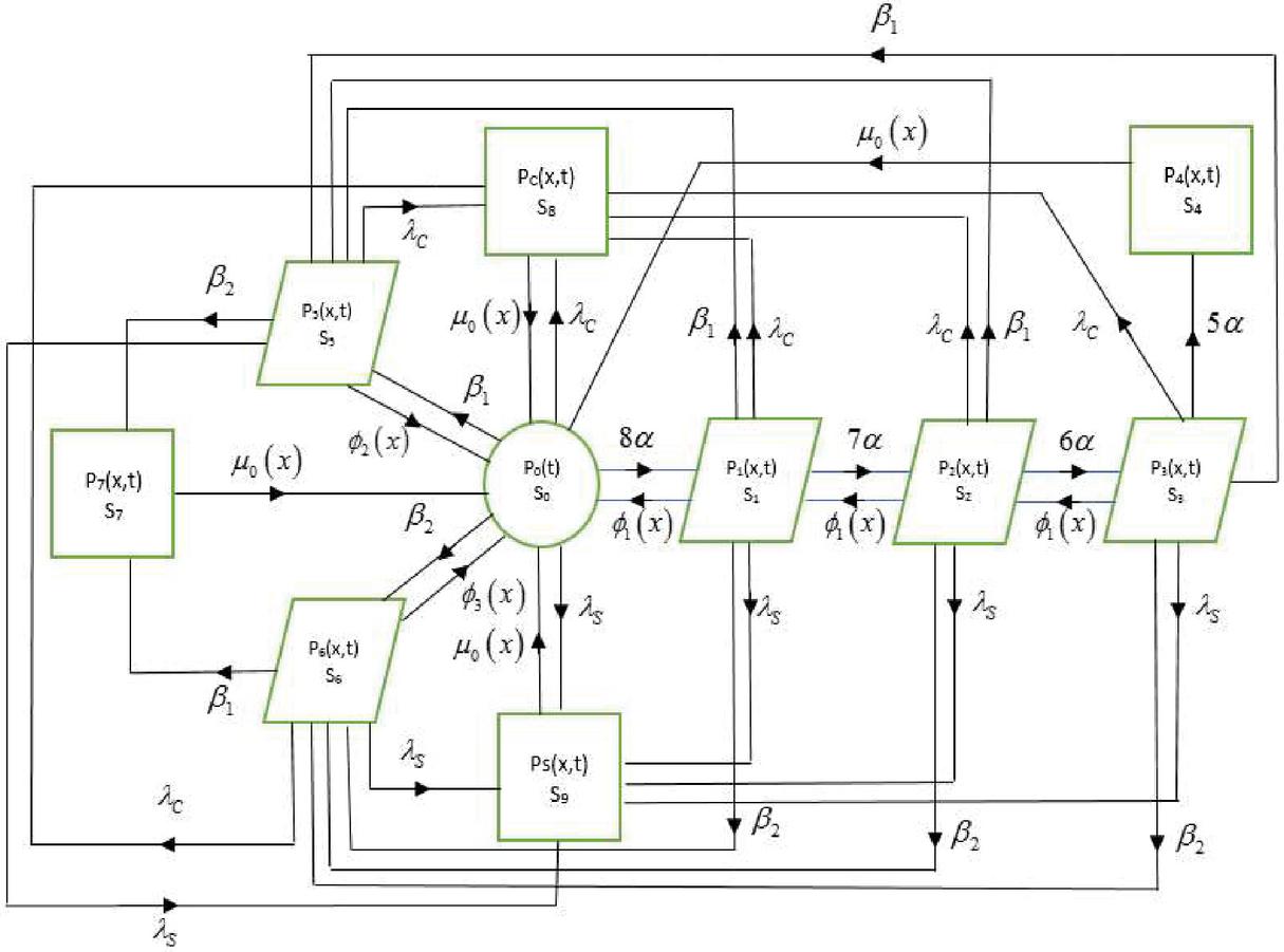
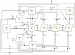
The paper is designed in six sections as follows: Section-2 labels the summary of system explanation together with assumptions and nomenclature. Section 3 consists of state description, system configuration and transition diagram. In Section 4 differential equations are developed with boundary conditions and then find the solutions. The results of the system performance like reliability, availability, MTTF, sensitivity and expected profit are given in Section 5. Results and conclusion with explanations are offered in Section 6 with the help of graphs. All the solutions including inverse Laplace transformation are obtained with help of MAPLE software. System configuration of the model is shown in Figure 1(a) and state transition diagram in Figure 1(b).

2.2 Assumptions

The following assumptions are made through this paper:

1. Initially the system is in state S${}_0$ and all the computer labs including two servers and switch are working perfectly.

2. There are eight computer labs in the system that are working under the policy 5-out-of-8: G, two non-identical data servers working under the policy 1-out-of-2: G and a switch that may be imperfect at the time of need.

3. The repairman is on-call around the clock and can be contacted as soon as the system fails completely or partially.

4. The failure rate of all the computer labs is the same and the database servers are different, but all the failure rates are constant in nature and follow exponential distribution.

5. Partially failed states can be repaired using a general repair policy, whereas completely failed states must be repaired right away for that the Goumbel-Hougard family copula repair policy can be implemented.

6. When a unit’s repair is finished, it becomes an active standby unit again (almost new). During the repair, there appears to be no harm.

2.3 Nomenclature

$s$, $t$	Laplace transform/Time scale variable.
$\alpha /{\beta }_1/{\beta }_2/{\lambda }_S/{\lambda }_C$	Failure rate of a computer lab/failure rate of server-1/ failure rate of server-2/failure rate of switch/failure rate due to catastrophic failure.
${\varphi }_1(x)/{\varphi }_2(x)/{\varphi }_3(x)$	Repair rate of a computer lab/repair rate of server-1/ repair rate of server-2 for supplementary variable $x$.
$P_i(t)$	The state transition probabilities that the system is in state $S_i$ for $i=0$ to 9.
$\overline{P}(s)$	Laplace transformation of the state transition probability $P(t)$.
$P_i(x,t)$	The probability that the system is in the state $S_i$ for $i=1\sim 9$ with elapsed repair time is $x$. $x$ is repair variable and $t$ is time variable.
$E_p(t)$	Expected profit in the interval $[0,t)$.
$K_1,K_2$	Revenue generated and service cost per unit time, respectively.
$S_{\varphi }(x)$	Notation function $S_{\varphi }(x)=\varphi (x)e^{-{\int }_0^x\varphi (x)\mathit{d}x}$ with repair distribution $\varphi (x)$.
${\overline{S}}_{\varphi }(s)$	Laplace transform of $S_{\varphi }(x)$ i.e. ${\overline{S}}_{\varphi }(x)={\int }_0^{\mathrm{\infty }}{e}^{-sx}\varphi (x)e^{-{\int }_0^x\varphi (x)\mathit{d}x}$.
${\mu }_0(x)$	Repair rate for completely failed states for supplementary variable $x$. It is joint probability function by Goumbel-Hougard copula family from complete failed state S${}_i$ to S${}_0$.

3 System Configuration and State Transition Diagram

In transition diagram, S${}_0$ is perfect state, S${}_1$, S${}_2$, S${}_3$, S${}_5$ and S${}_6$ partial failed/degraded and S${}_4$, S${}_7$, S${}_8$ and S${}_9$ are completely failed states. The system approach to S${}_1$, S${}_2$ and S${}_3$ due to failure of one, two or three computer labs respectively. The transitions approach to S${}_5$ or S${}_6$ after failing first or second server respectively. The state S${}_4$ and S${}_7$ are completely failed states due to failure of more than 4 computer labs and both the servers respectively, while S${}_8$ is completely failed state due to switch failure. The state S${}_9$ is completely failed due to catastrophic failure.

Figure 1(a): System configuration of the model.

Figure 1(b): State transition diagram of the model.

4 Formulation of Mathematical Model

By probability of considerations and continuity arguments, we can obtain the following set of difference-differential equations associated with the present mathematical model.

$\left[{\displaystyle \frac{\partial }{\partial t}}+8\alpha +{\beta }_1+{\beta }_2+{\lambda }_S+{\lambda }_C\right]P_0(t)$

$\mathrm{\hspace{1em}\hspace{1em}}={\displaystyle {\int }_0^{\mathrm{\infty }}}{\varphi }_1(x)P_1(x,t)\mathit{d}x+{\displaystyle {\int }_0^{\mathrm{\infty }}}{\varphi }_2(x)P_5(x,t)\mathit{d}x$

$\mathrm{\hspace{1em}\hspace{1em}}\mathit{\hspace{1em}}+{\displaystyle {\int }_0^{\mathrm{\infty }}}{\varphi }_3(x)P_6(x,t)\mathit{d}x+{\displaystyle {\int }_0^{\mathrm{\infty }}}{\mu }_0(x)P_i(x,t)\mathit{d}x;i=4,7,c,s$

$\left[{\displaystyle \frac{\partial }{\partial t}}+{\displaystyle \frac{\partial }{\partial x}}+7\alpha +{\beta }_1+{\beta }_2+{\lambda }_S+{\lambda }_C+{\varphi }_1(x)\right]P_1(x,t)=0$

$\left[{\displaystyle \frac{\partial }{\partial t}}+{\displaystyle \frac{\partial }{\partial x}}+6\alpha +{\beta }_1+{\beta }_2+{\lambda }_S+{\lambda }_C+{\varphi }_1(x)\right]P_2(x,t)=0$

$\left[{\displaystyle \frac{\partial }{\partial t}}+{\displaystyle \frac{\partial }{\partial x}}+5\alpha +{\beta }_1+{\beta }_2+{\lambda }_S+{\lambda }_C+{\varphi }_1(x)\right]P_3(x,t)=0$

$\left[{\displaystyle \frac{\partial }{\partial t}}+{\displaystyle \frac{\partial }{\partial x}}+{\beta }_2+{\lambda }_S+{\lambda }_C+{\varphi }_2(x)\right]P_5(x,t)=0$

$\left[{\displaystyle \frac{\partial }{\partial t}}+{\displaystyle \frac{\partial }{\partial x}}+{\beta }_1+{\lambda }_S+{\lambda }_C+{\varphi }_3(x)\right]P_6(x,t)=0$

$[{\displaystyle \frac{\partial }{\partial t}}+{\displaystyle \frac{\partial }{\partial x}}+\exp {[x^{\theta }+{\left\{\log \varphi (x)\right\}}^{\theta }]}^{1/\theta }]P_j(x,t)=0;j=4,7,c,s$

Boundary conditions

$P_1(0,t)$	$=8\alpha P_0(t)$
$P_2(0,t)$	$=7\alpha P_1(0,t)=56{\alpha }^2{P}_0(t)$
$P_3(0,t)$	$=6\alpha P_2(0,t)=336{\alpha }^3{P}_0(t)$
$P_4(0,t)$	$=5\alpha P_3(0,t)=1680{\alpha }^4{P}_0(t)$
$P_5(0,t)$	$={\beta }_1[P_0(t)+P_1(0,t)+P_2(0,t)+P_3(0,t)]$
$P_6(0,t)$	$={\beta }_2[P_0(t)+P_1(0,t)+P_2(0,t)+P_3(0,t)]$
$P_7(0,t)$	$={\beta }_1{P}_6(0,t)+{\beta }_2{P}_5(0,t)$
$P_S(0,t)$	$={\lambda }_S[P_0(t)+P_1(0,t)+P_2(0,t)$
	$\mathrm{\hspace{1em}}+P_3(0,t)+P_5(0,t)+P_6(0,t)]$
$P_C(0,t)$	$={\lambda }_C[P_0(t)+P_1(0,t)+P_2(0,t)$
	$\mathrm{\hspace{1em}}+P_3(0,t)+P_5(0,t)+P_6(0,t)]$

Initial conditions

$$P_0(0)=1,\text{ and other state probabilities are zero at }t=0$$

(1)

Solution of the model.

Taking Laplace transformation of all the above equations using Equation (1), we obtain

$[s+8\alpha +{\beta }_1+{\beta }_2+{\lambda }_S+{\lambda }_C]{\overline{P}}_0(s)$

$\mathrm{\hspace{1em}\hspace{1em}}=1+{\displaystyle {\int }_0^{\mathrm{\infty }}}{\varphi }_1(x){\overline{P}}_1(x,s)\mathit{d}x+{\displaystyle {\int }_0^{\mathrm{\infty }}}{\varphi }_2(x){\overline{P}}_5(x,s)\mathit{d}x$

$\mathrm{\hspace{1em}\hspace{1em}}\mathit{\hspace{1em}}+{\displaystyle {\int }_0^{\mathrm{\infty }}}{\varphi }_3(x){\overline{P}}_6(x,s)\mathit{d}x+{\displaystyle {\int }_0^{\mathrm{\infty }}}{\mu }_0(x){\overline{P}}_i(x,s)\mathit{d}x;i=4,7,c,s$

$\left[s+{\displaystyle \frac{\partial }{\partial x}}+7\alpha +{\beta }_1+{\beta }_2+{\lambda }_S+{\lambda }_C+{\varphi }_1(x)\right]{\overline{P}}_1(x,s)=0$

$\left[s+{\displaystyle \frac{\partial }{\partial x}}+6\alpha +{\beta }_1+{\beta }_2+{\lambda }_S+{\lambda }_C+{\varphi }_1(x)\right]{\overline{P}}_2(x,s)=0$

$\left[s+{\displaystyle \frac{\partial }{\partial x}}+5\alpha +{\beta }_1+{\beta }_2+{\lambda }_S+{\lambda }_C+{\varphi }_1(x)\right]{\overline{P}}_3(x,s)=0$

$\left[s+{\displaystyle \frac{\partial }{\partial x}}+{\beta }_2+{\lambda }_S+{\lambda }_C+{\varphi }_2(x)\right]{\overline{P}}_5(x,s)=0$

$\left[s+{\displaystyle \frac{\partial }{\partial x}}+{\beta }_1+{\lambda }_S+{\lambda }_C+{\varphi }_3(x)\right]{\overline{P}}_6(x,s)=0$

$[s+{\displaystyle \frac{\partial }{\partial x}}+\exp {[x^{\theta }+{\left\{\log \varphi (x)\right\}}^{\theta }]}^{1/\theta }]{\overline{P}}_j(x,s)=0;j=4,7,c,s$

Boundary conditions

${\overline{P}}_1(0,s)$	$=8\alpha {\overline{P}}_0(s)$
${\overline{P}}_2(0,s)$	$=7\alpha {\overline{P}}_1(0,s)=56{\alpha }^2{\overline{P}}_0(s)$
${\overline{P}}_3(0,s)$	$=6\alpha {\overline{P}}_2(0,s)=336{\alpha }^3{\overline{P}}_0(s)$
${\overline{P}}_4(0,s)$	$=5\alpha {\overline{P}}_3(0,s)=1680{\alpha }^4{\overline{P}}_0(s)$
${\overline{P}}_5(0,s)$	$={\beta }_1\left(1+8\alpha +56{\alpha }^2+336{\alpha }^3\right){\overline{P}}_0(s)$
${\overline{P}}_6(0,s)$	$={\beta }_2\left(1+8\alpha +56{\alpha }^2+336{\alpha }^3\right){\overline{P}}_0(s)$
${\overline{P}}_7(0,s)$	$={\beta }_1{\overline{P}}_6(0,s)+{\beta }_2{\overline{P}}_5(0,s)$
	$=2{\beta }_1{\beta }_2\left(1+8\alpha +56{\alpha }^2+336{\alpha }^3\right){\overline{P}}_0(s)$
${\overline{P}}_S(0,s)$	$={\lambda }_S\left(1+{\beta }_1+{\beta }_2\right)\left(1+8\alpha +56{\alpha }^2+336{\alpha }^3\right){\overline{P}}_0(s)$
${\overline{P}}_C(0,s)$	$={\lambda }_C\left(1+{\beta }_1+{\beta }_2\right)\left(1+8\alpha +56{\alpha }^2+336{\alpha }^3\right){\overline{P}}_0(s)$

Laplace transformation of boundary conditions after repair

${\overline{P}}_1(0,s)$	$={\displaystyle \frac{8\alpha }{1-7\alpha {\overline{S}}_{{\varphi }_1}\left(s+6\alpha +{\beta }_1+{\beta }_2+{\lambda }_S+{\lambda }_C\right)}}{\overline{P}}_0(s)$
	$={\displaystyle \frac{8\alpha }{1-7\alpha P}}{\overline{P}}_0(s)$
${\overline{P}}_2(0,s)$	$={\displaystyle \frac{56{\alpha }^2}{1-6\alpha {\overline{S}}_{{\varphi }_1}\left(s+5\alpha +{\beta }_1+{\beta }_2+{\lambda }_S+{\lambda }_C\right)}}{\overline{P}}_0(s)$
	$={\displaystyle \frac{56{\alpha }^2}{1-6\alpha Q}}{\overline{P}}_0(s)$

Solving all the above equations with the implications of boundary conditions and ${\overline{P}}_i(s)={\int }_0^{\mathrm{\infty }}{\overline{P}}_i(x,s)\mathit{d}x$ we may get Laplace transform of state transition probabilities as:

${\overline{P}}_0(s)$	$={\displaystyle \frac{1}{D(s)}}$	(2)
${\overline{P}}_1(s)$	$={\displaystyle \frac{8\alpha }{D(s)}}{\displaystyle \frac{1-R}{\left(s+7\alpha +{\beta }_1+{\beta }_2+{\lambda }_S+{\lambda }_C\right)\left(1-7\alpha P\right)}}$	(3)
${\overline{P}}_2(s)$	$={\displaystyle \frac{56{\alpha }^2}{D(s)}}{\displaystyle \frac{1-P}{\left(s+6\alpha +{\beta }_1+{\beta }_2+{\lambda }_S+{\lambda }_C\right)\left(1-6\alpha Q\right)}}$	(4)
${\overline{P}}_3(s)$	$={\displaystyle \frac{336{\alpha }^3}{D(s)}}{\displaystyle \frac{1-Q}{\left(s+5\alpha +{\beta }_1+{\beta }_2+{\lambda }_S+{\lambda }_C\right)}}$	(5)
${\overline{P}}_4(s)$	$={\displaystyle \frac{1680{\alpha }^4}{D(s)}}{\displaystyle \frac{1-U}{s}}$	(6)
${\overline{P}}_5(s)$	$={\displaystyle \frac{{\beta }_1\left(1+8\alpha +56{\alpha }^2+336{\alpha }^3\right)}{D(s)}}{\displaystyle \frac{1-S}{\left(s+{\beta }_2+{\lambda }_S+{\lambda }_C\right)}}$	(7)
${\overline{P}}_6(s)$	$={\displaystyle \frac{{\beta }_2\left(1+8\alpha +56{\alpha }^2+336{\alpha }^3\right)}{D(s)}}{\displaystyle \frac{1-T}{\left(s+{\beta }_1+{\lambda }_S+{\lambda }_C\right)}}$	(8)
${\overline{P}}_7(s)$	$={\displaystyle \frac{2{\beta }_1{\beta }_2\left(1+8\alpha +56{\alpha }^2+336{\alpha }^3\right)}{D(s)}}{\displaystyle \frac{1-U}{s}}$	(9)
${\overline{P}}_S(s)$	$={\displaystyle \frac{{\lambda }_S\left(1+{\beta }_1+{\beta }_2\right)\left(1+8\alpha +56{\alpha }^2+336{\alpha }^3\right)}{D(s)}}{\displaystyle \frac{1-U}{s}}$	(10)
${\overline{P}}_C(s)$	$={\displaystyle \frac{{\lambda }_C\left(1+{\beta }_1+{\beta }_2\right)\left(1+8\alpha +56{\alpha }^2+336{\alpha }^3\right)}{D(s)}}{\displaystyle \frac{1-U}{s}}$	(11)

Where

$D(s)$	$=s+8\alpha +{\beta }_1+{\beta }_2+{\lambda }_S+{\lambda }_C-{\displaystyle \frac{8\alpha R}{1-7\alpha P}}$
	$\mathrm{\hspace{1em}}-(1+8\alpha +56{\alpha }^2+336{\alpha }^3)({\beta }_{1}S+{\beta }_{2}T)$
	$\mathrm{\hspace{1em}}-U\{1680{\alpha }^4+(1+8\alpha +56{\alpha }^2+336{\alpha }^3)$
	$\mathrm{\hspace{1em}\hspace{1em}}\mathit{\hspace{1em}\hspace{1em} }(2{\beta }_1{\beta }_2+({\lambda }_S+{\lambda }_C)(1+{\beta }_1+{\beta }_2))\}$
$P$	$={\overline{S}}_{{\varphi }_1}\left(s+6\alpha +{\beta }_1+{\beta }_2+{\lambda }_S+{\lambda }_C\right)$
	$={\displaystyle \frac{{\varphi }_1}{s+6\alpha +{\beta }_1+{\beta }_2+{\lambda }_S+{\lambda }_C+{\varphi }_1}}$
$Q$	$={\overline{S}}_{{\varphi }_1}(s+5\alpha +{\beta }_1+{\beta }_2+{\lambda }_S+{\lambda }_C)$
	$={\displaystyle \frac{{\varphi }_1}{s+5\alpha +{\beta }_1+{\beta }_2+{\lambda }_S+{\lambda }_C+{\varphi }_1}}$
$R$	$={\overline{S}}_{{\varphi }_1}(s+7\alpha +{\beta }_1+{\beta }_2+{\lambda }_S+{\lambda }_C)$
	$={\displaystyle \frac{{\varphi }_1}{s+7\alpha +{\beta }_1+{\beta }_2+{\lambda }_S+{\lambda }_C+{\varphi }_1}}$
$S$	$={\overline{S}}_{{\varphi }_2}(s+{\beta }_2+{\lambda }_S+{\lambda }_C)={\displaystyle \frac{{\varphi }_2}{s+{\beta }_2+{\lambda }_S+{\lambda }_C+{\varphi }_2}}$
$T$	$={\overline{S}}_{{\varphi }_3}(s+{\beta }_1+{\lambda }_S+{\lambda }_C)={\displaystyle \frac{{\varphi }_3}{s+{\beta }_1+{\lambda }_S+{\lambda }_C+{\varphi }_3}}$
$\text{and}\mathit{\hspace{1em}}U$	$={\overline{S}}_{{\mu }_0}(s)={\displaystyle \frac{{\mu }_0}{s+{\mu }_0}}$

Sum of Laplace transformations of the state transitions, where the system is in operational mode, is as follows

$${\overline{P}}_{up}(s)={\overline{P}}_0(s)+{\overline{P}}_1(s)+{\overline{P}}_2(s)+{\overline{P}}_3(s)+{\overline{P}}_5(s)+{\overline{P}}_6(s)$$

(12)

5 Analytical Study

5.1 Availability Analysis

To evaluate availability, let us consider two different cases for repair of the computer labs (i) general repair and (ii) Gumbel-Hougaard family copula repair. Let us fix the Laplace transforms as

${\overline{S}}_{{\mu }_0}(s)$	$={\overline{S}}_{\exp {[x^{\theta }+{\{\log \varphi (x)\}}^{\theta }]}^{1/\theta }}(s)={\displaystyle \frac{\exp {[x^{\theta }+{\{\log \varphi (x)\}}^{\theta }]}^{1/\theta }}{s+\exp {[x^{\theta }+{\{\log \varphi (x)\}}^{\theta }]}^{1/\theta }}}\mathit{\hspace{1em}}\text{and}$
${\overline{S}}_{{\alpha }_i}(s)$	$={\displaystyle \frac{{\alpha }_i}{s+{\alpha }_i}},i=1,2,3.$

Taking the values of different parameters of failure rates as $\alpha =0.02$, ${\beta }_1=0.03,{\beta }_2=0.031,{\lambda }_S=0.025,$ ${\lambda }_C=0.1$ and $x=1$.

Case-I: Taking repair rates as ${\varphi }_i(x)=1(i=1\sim 3)$ and ${\mu }_0=2.718$ in Equation (12). After taking inverse Laplace transformation, one may get the expression for availability under copula repair as

$P_{up}(t)$	$=0.3548e^{-1.2860t}+0.0598e^{-2.8996t}-0.0402e^{-1.3814t}$
	$\mathrm{\hspace{1em}}-0.3617e^{-1.2862t}+0.0003e^{-1.1589t}$
	$\mathrm{\hspace{1em}}+6.0759{10}^{-6}{e}^{-1.1554t}+0.9912e^{-0.0151t}-0.0042e^{-1.3060t}$	(13)

Case-II: Taking repair rates as ${\varphi }_i(x)=1(i=1\sim 3)$ and ${\mu }_0=1$ in Equation (12). After taking inverse Laplace transformation, one may get the expression for availability under general repair as

$P_{up}(t)$	$=0.0283e^{-1.4859t}-0.0377e^{-1.3070t}-0.0005e^{-1.1591t}$
	$\mathrm{\hspace{1em}}-0.0477e^{-1.0574t}+0.9136e^{-0.0139t}$
	$\mathrm{\hspace{1em}}+1.0513{10}^{-5}{e}^{-1.1554t}+0.0031e^{-1.2860t}-0.0444e^{-1.3060t}$	(14)

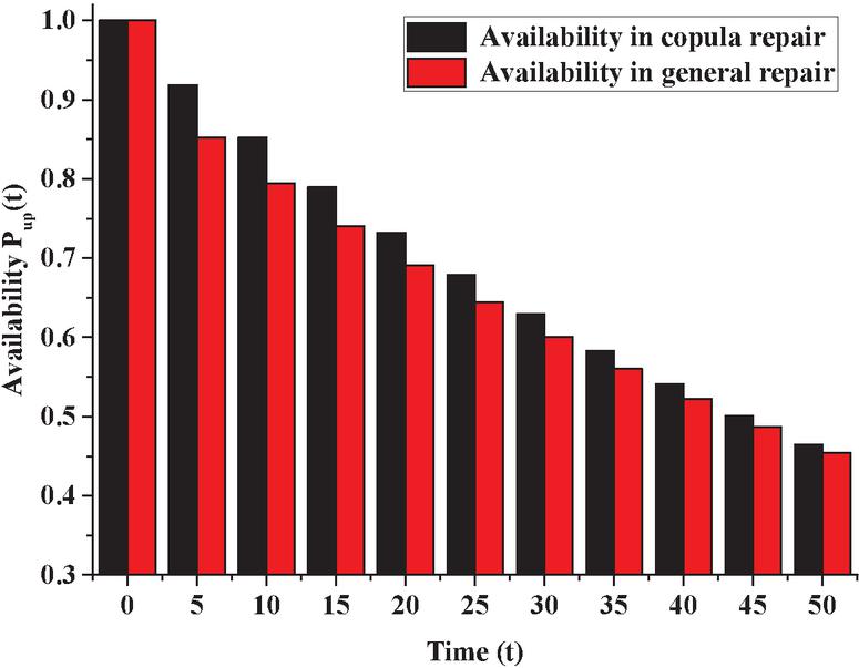
Fixing values of time variable as $t=0$,5,10,15,20,25,30,35,40,45 and 50 units of time in Equations (13) and (14). The comparison between the two cases for availability $P_{up}(t)$ is presented in Figure 2.

Figure 2 Comparison in availabilities w.r.t time under different repair policies.

5.2 Reliability of the System

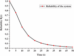
Reliability is the probability that the system will perform its intended function for a given period. It is obtained by putting all repair rates to zero and then obtain inverse Laplace transform of Equation (12). An expression for the reliability of the system after fixing the failure rates as $\alpha =0.02,$ ${\beta }_1=0.03,{\beta }_2=0.031,{\lambda }_S=0.025,{\lambda }_C=0.1$ may be obtain as –

$R_i(t)$	$=0.1871e^{-0.0560t}+0.0448e^{-0.1860t}-0.5600e^{-0.2060t}$
	$\mathrm{\hspace{1em}}-8.0000e^{-0.2260t}+7.9842e^{-0.2460t}+0.1923e^{-0.0550t}$	(15)

Fixing values of time variable as $t=0$,5,10,15,20,25,30,35,40,45 and 50 units of time in Equation (15), we can get different values of $R_i(t)$ with the help of (15) as shown in Figure 3.

Figure 3 Variation in reliability with respect to time.

5.3 Mean Time to Failure (MTTF)

The mean time to failure indicates how long an item is expected to function before failing and it can be obtained by taking all repair rates to zero i.e. ${\varphi }_1={\varphi }_2={\varphi }_3={\mu }_0=0$ and the limit as s tends to zero in Equation (12) for the exponential distribution, we can obtain the MTTF as:

$\mathit{MTTF}$	$={\displaystyle \frac{1}{A}}[1+{\displaystyle \frac{8\alpha }{(A-\alpha )}}+{\displaystyle \frac{56{\alpha }^2}{(A-2\alpha )}}+{\displaystyle \frac{336{\alpha }^3}{(A-3\alpha )}}$
	$\mathrm{\hspace{1em}}+{\displaystyle \frac{{\beta }_{1}B}{({\beta }_2+{\lambda }_S+{\lambda }_C)}}+{\displaystyle \frac{{\beta }_{2}B}{({\beta }_1+{\lambda }_S+{\lambda }_C)}}]$	(16)

where $A=8\alpha +{\beta }_1+{\beta }_2+{\lambda }_S+{\lambda }_C$ and $B=1+8\alpha +56{\alpha }^2+336{\alpha }^3$.

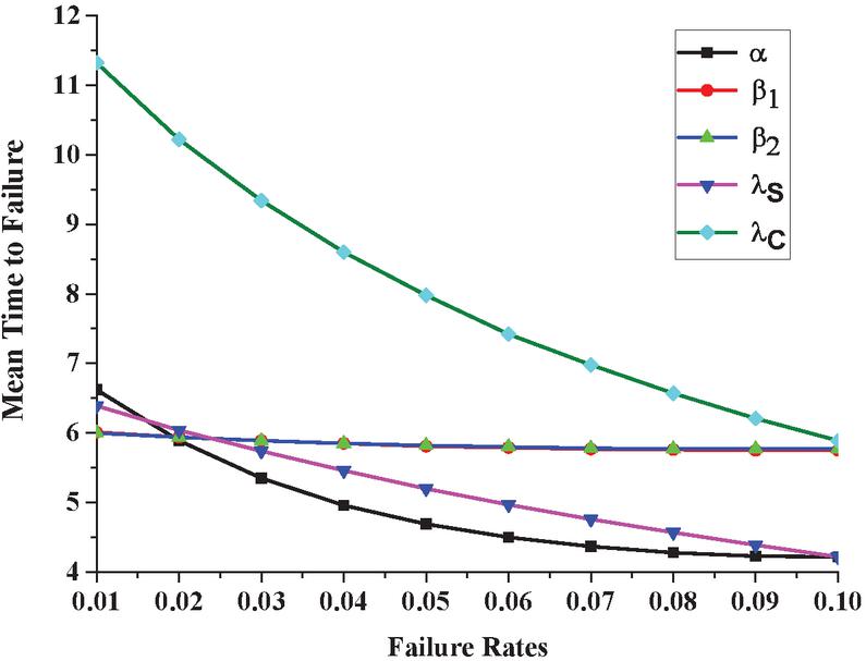
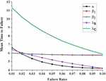
By taking the different values of parameters as $\alpha =0.02,{\beta }_1=0.03,{\beta }_2=0.031,{\lambda }_S=0.025,{\lambda }_C=0.1$ and varying $\alpha ,{\beta }_1,{\beta }_2,{\lambda }_S$ and ${\lambda }_C$ one by one by fixing values as 0.01, 0.02, 0.03, 0.04, 0.05, 0.06, 0.07, 0.08, 0.09 and 0.10 in Equation (16). The variation in MTTF w.r.t. failure rate can be obtained in Figure 4.

Figure 4 MTTF as a function of failure rates.

5.4 Sensitivity Variation of the System

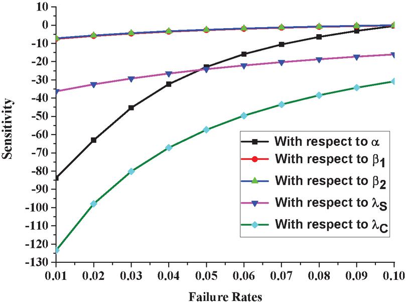
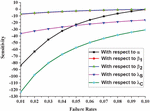
The effect of modeling parameters on a system’s expected dependability is measured through sensitivity analysis. The partial differentiation of the mean time to failure regarding the system’s failure rates can be used to determine sensitivity. Setting the parameters as $\alpha =0.02,{\beta }_1=0.03,{\beta }_2=0.031$, ${\lambda }_S=0.025$, and ${\lambda }_C=0.1$ in the partial differentiation of Equation (16) obtained using Maple, we get the sensitivity of the system as shown in Figure 5.

Figure 5 Variation in sensitivity in MTTF corresponding to failure rates.

5.5 Cost Analysis

Let the failure rates are $\alpha =0.02,{\beta }_1=0.03,{\beta }_2=0.031,$ ${\lambda }_S=0.025$, ${\lambda }_C=0.1$ and $x=1$ and the service facility be constantly available, then the expected profit during the interval $[0,t)$ is

$$E_p(t)=K_1{\int }_0^t{P}_{up}(t)\mathit{d}t-K_{2}t$$

Where K${}_1$ and K${}_2$ are service and revenue costs per unit of time.

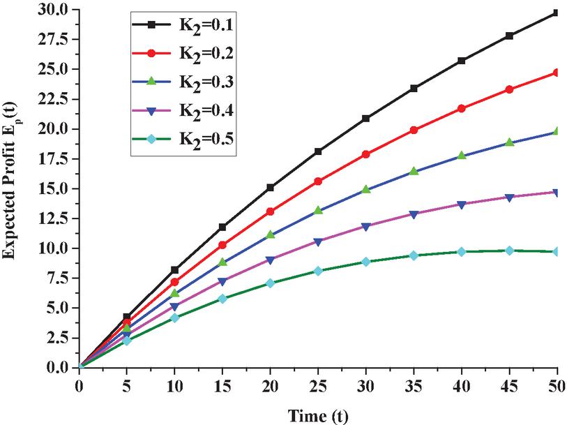
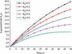
Figure 6 Expected profit E${}_{\mathrm{p}}$(t) under copula repair w.r.t time t.

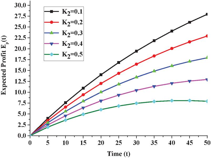
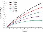
Figure 7 Expected profit E${}_{\mathrm{p}}$(t) under general repair w.r.t time t.

Figure 8 Comparison in expected profit for copula Vs general repair for K${}_2=0.1$.

Then the expected profit incurred during $[0,t)$ under copula repair is –

$R_i(t)$	$=K_1\{65.37-0.0206e^{-2.8996t}+0.2812e^{-1.2862t}$
	$\mathrm{\hspace{1em}}-5.2584{10}^{-6}{e}^{-1.1554t}+0.0291e^{-1.3814t}$
	$\mathrm{\hspace{1em}}-0.0002e^{-1.1589t}-65.39e^{-0.0151t}+0.0032e^{-1.3060t}$
	$\mathrm{\hspace{1em}}-0.2759e^{-1.2860t}\}-K{}_{2}t$	(17)

and profit incurred under general repair is –

$R_i(t)$	$=K_1\{65.37-0.0190e^{-1.4859t}+0.0289e^{-1.3070t}$
	$\mathrm{\hspace{1em}}-9.0988{10}^{-6}{e}^{-1.1555t}-0.0004e^{-1.1591t}$
	$\mathrm{\hspace{1em}}-0.0452e^{-1.0573t}-65.31e^{-0.0139t}-0.0340e^{-1.3060t}$
	$\mathrm{\hspace{1em}}-0.0024e^{-1.2860t}\}-K{}_{2}t$	(18)

Fixing revenue cost K${}_1$ at 1 and varying service cost K${}_2$ as 0.1, 0.2, 0.3, 0.4 and 0.5 and changing the time as $t=0$,5,10,15,20,25,30,35,40,45 and 50 in Equations (17) and (18), one can see the expected profit under copula repair in Figure 6 and expected profit under general repair in Figure 7. A comparison in expected profit for copula and general repair for K${}_2=0.1$ can be seen in Figure 8. Similar comparisons can be made for other values of K${}_2$.

6 Results and Conclusion

This paper studies the reliability characteristics of a computer lab network system consisting of eight computer labs working on 5-out-of-8: G policy, two non-identical data servers working on 1-out-of-2: G policy and a switch. The system may experience catastrophic failure due to unwanted circumstances like software failure, power failure, hardware failure etc. The authors utterances the following important observations:

1. Figure 2 provides information on availability under copula repair Vs general repair with respect to time when we fixed failure parameters at $\alpha =0.02,{\beta }_1=0.03,{\beta }_2=0.031,{\lambda }_S=0.025$ and ${\lambda }_C=0.1$. It can be revealed from the graph that availability decreases as time increases. Moreover, the availability is better in case of copula repair as compared to general repair, which shows that the decision managers may opt for copula repair as it gives better performance.

2. The reliability of the system can be revealed from Figure 3 for the same set of parameters except all type of repairs are zero. One can easily conclude that reliability is decreasing sharply for higher values of t and with the passage of time, ultimately it becomes zero. Undoubtedly, the availability is far better than reliability for various values of t, which indicates the requirement for repairing of the system.

3. Figure 4 shows the graph of MTTF Vs failure rates $\alpha ,{\beta }_1,{\beta }_2,{\lambda }_S$ and ${\lambda }_C$. Observation revealed that MTTF is same for ${\beta }_1$ and ${\beta }_2$, lower for $\alpha$ and higher for ${\lambda }_C$. However, in all the five cases it decreases as the failure rate increases and stabilizes for higher values of $\alpha ,{\beta }_1,{\beta }_2,{\lambda }_S$ and ${\lambda }_C$.

4. The sensitivities of the system reliability with respect to $\alpha ,{\beta }_1,{\beta }_2,{\lambda }_S$ and ${\lambda }_C$ can be depicted in Figure 5 while varying all from 0.01 to 0.10. We perceive that sensitivity is almost same for ${\beta }_1$ and ${\beta }_2$ as compared to ${\lambda }_C$. Furthermore, the influence of $\alpha$ and ${\lambda }_C$ on the system reliability increases more as $\alpha$ and ${\lambda }_C$ increases. We observe that system reliability is more sensitive with respect to $\alpha$.

5. The variation in expected profit under copula repair for various t is presented in Figure 6 and with respect to general repair in Figure 7. A comparison in expected profit for copula and general repair for service cost K${}_2=0.1$ can be seen in Figure 8. By observations from the figure, one can see that expected profit reduces as the service cost increases from 0.1 to 0.6 with respect to time. Besides this, the expected profit is higher if we repair the system via copula repair.

In comparison to some previous publications, the results are more thorough and improved. The use of an additional security server is anticipated for future work, as data servers are focused on gathering, storing, processing, allocating, or granting access to massive amounts of data.

References

[1] Deswal, S. and Malik, S. C. (2015). Reliability measures of a system of two non-identical units with priority subject to weather conditions. Journal of Reliability and Statistical Studies, 8(1), 181–190.

[2] Ding, Y., Lin, Y., Peng, R. and Zuo, M.J. (2019). Approximate Reliability Evaluation of Large-Scale Multistate Series-Parallel Systems. IEEE Transactions on Reliability, 68(2), 539–553.

[3] Goyal, N., Ram, M., Amoli, S. and Suyal, A. (2017). Sensitivity analysis of a three-unit series system under K-out-of-n redundancy. International Journal of Quality and Reliability Management, 34(6), 770–784.

[4] Ismail, A.L., Abdullahi, S. and Yusuf, I. (2022). Performance evaluation of a hybrid series–parallel system with two human operators using Gumbel–Hougaard family copula. International Journal of Quality & Reliability Management, 39(1), 297–315.

[5] Jibril, A.B., Singh, V.V. and Rawal, D.K. (2022). Probabilistic assessment of complex system consisting three subsystems, multi-failure threats and copula repair approach. International Journal of Quality & Reliability Management, doi: 10.1108/IJQRM-03-2021-0061.

[6] Kadyan, S., Malik S. C. and Gitanjali (2020). Stochastic Analysis of a Three-Unit Non-Identical Repairable System with Simultaneous Working of Cold Standby Units. Journal of Reliability and Statistical Studies, 13(2–4), 385–400.

[7] Kızılaslan, F. (2021). Stochastic comparisons of series and parallel systems with independent heterogeneous Gumbel and truncated Gumbel components”, International Journal of Quality & Reliability Management, 38(8), 1771–1791.

[8] Kumar, A. and Kumar, P. (2020). Application of Markov process/mathematical modelling in analysing communication system reliability. International Journal of Quality & Reliability Management, 37(2), 354–371.

[9] Kumar, D. and Singh, S.B. (2016). Stochastic analysis of the complex repairable system with deliberate failure emphasizing reboot delay. Communication in Statistics – Simulation and Computation, 45(2), 1–20.

[10] Lin, Y.K. (2007). Reliability evaluation for an information network with node failure under cost constraint. IEEE Trans. Syst., Man, Cybern. - Part A: Syst., Humans, 37(2), 180–188.

[11] Lin, Y.K. (2010). Evaluation of network reliability for a computer network subject to a budget constraint. International Journal of Innovative Computing, Information and Control, 59(3), 539–550.

[12] Lin, Y.K. and Yeng, L.C. (2012). Evaluation of Network Reliability for Computer Networks with Multiple Sources. Mathematical Problems in Engineering, vol. 2012, Article ID 737562, 18 pages.

[13] Malik S.C., Bhardwaj R. K. and Grewal A. S. (2010). Probabilistic analysis of a system of two non-identical parallel units with priority to repair subject to inspection, Journal of Reliability and Statistical Studies, 3(1), 1–11.

[14] Munjal, A. and Singh, S. B. (2014). Reliability analysis of a complex repairable system composed of a 2-out-of-3: G subsystem and a series subsystem connected in parallel. Journal of Reliability and Statistical Studies, 7, 19–39.

[15] Nailwal, B. and Singh, S. B. (2012). Reliability measures and sensitivity analysis of a Complex matrix system including power failure, IJE Transactions A: Basics, 25(2), 115–130.

[16] Nautiyal, N., Singh, S.B. and Bisht, S. (2020). Analysis of reliability and its characteristics of a k-out-of-n network incorporating copula. International Journal of Quality & Reliability Management, 37(4), 517–537.

[17] Negi, S. and Singh, S. B. (2015). Reliability analysis of non-repairable complex system with weighted subsystems connected in series. Applied Mathematics and Computation, 262, 79–89.

[18] Niaki, S.T.A. and Yaghoubi, A. (2021). Exact equations for the reliability and mean time to failure of 1-out-of-N cold standby system with imperfect switching. J. Optim. Indus. Eng. 14(2), 197–203.

[19] Poonia, P.K. (2022). Exact reliability formula for n-clients computer network with catastrophic failure and copula repair. Int. J. of Computing Science and Mathematics. (In press).

[20] Poonia, P.K. (2021). Performance assessment of a multi-state computer network system in series configuration using copula repair. Int. J. Reliability and Safety, 15(1/2), 68–88.

[21] Poonia, P.K., Sirohi, A. and Kumar, A. (2021). Cost analysis of a repairable warm standby k-out-of-n: G and 2-out-of-4: G systems in series configuration under catastrophic failure using copula repair. Life Cycle Reliab Saf Eng., 10(2), 121–133.

[22] Qiu, Q. and Cui, L. (2019). Availability analysis for general repairable systems with repair time threshold. Communications in Statistics – Theory and Methods, 48(3), 1–20.

[23] Ram, M. and Goyal, N. (2018). Bi-directional system analysis under copula-coverage approach. Communications in Statistics-Simulation and Computation, 47(6), 1831–1844.

[24] Renu, Bisht, S. and Singh, S. B. (2021). Reliability Evaluation of Repairable Parallel-Series Multi-State System Implementing Interval Valued Universal Generating Function. Journal of Reliability and Statistical Studies, 14(1), 81–120.

[25] Sanusi, A. and Yusuf, I. (2021). Cost analysis of 2-out-of-4 system connected to two-unit parallel supporting device for operation. Life Cycle Reliab Saf Eng, 10, 113–119.

[26] Sharma, R. and Kumar, G. (2017). Availability improvement for the successive K-out-of-n machining system using stand by with multiple working vacations. International Journal of Reliability and Safety, 11(3/4), 256–267.

[27] Singh, V.V., Gulati, J., Rawal, D.K. and Goel, C.K. (2016). Performance analysis of complex system in the series configuration under different failure and repair discipline using copula. International Journal of Reliability, Quality, and Safety Engineering, 23(2), 1–21.

[28] Singh, V.V. and Poonia, P. K. (2022). Stochastic analysis of k-out-of-n: G type of repairable system in combination of subsystems with controllers and multi repair approach, J. Optim. Indus. Eng., 15(1), 121–130.

[29] Tyagi, V., Arora, R., Ram, M., and Yadav, O.P. (2019). 2-Out-of-3: F System analysis under catastrophic failure. Nonlinear Studies, 26(3), 557–574.

[30] Yaghoubi, A., Niaki, S.T.A. and Rostamzadeh, H. (2020). A closed-form equation for steady-state availability of cold standby repairable k-out-of-n: G systems. International Journal of Quality & Reliability Management, 37(1), 145–155.

[31] Yeh, F.M., Lu, S.K. and Kuo, S.Y. (2002). Obdd-based evaluation of k-terminal network reliability. IEEE Transactions on Reliability, 51(4), 443–451.

[32] Yusuf, I. and Musa, I. M. (2021). Availability Enhancement of a Complex Hybrid System Consisting of Three Subsystems. Int. J. of Operations Research, 18(1), 1–9.

Biography

Praveen Kumar Poonia is presently working as Assistant Professor in the Department of General Requirements, University of Technology and Applied Sciences, Ibri College of Applied Sciences, Ibri, Sultanate of Oman. Previously he served as a professor at Bharat Institute of Technology, Meerut, India for sixteen years under Dr. APJ Abdul Kalam Technical University, India. He received his Ph. D degree in Mathematics from Chaudhary Charan Singh University, Meerut, UP, India in 2005. He has published several research papers in renowned international journals. His research interests include reliability theory and reliability modelling. He is reviewer in various highly respected journals in the areas of Reliability, Statistics, and Optimization. Dr. Poonia has been a member/life member of various academic/professional bodies.

Journal of Reliability and Statistical Studies, Vol. 15, Issue 1 (2022), 105–128.
doi: 10.13052/jrss0974-8024.1515
© 2022 River Publishers

Abstract

1 Introduction

2 Model Explanation and Notations

2.1 System Explanation

2.2 Assumptions

2.3 Nomenclature

3 System Configuration and State Transition Diagram

4 Formulation of Mathematical Model

5 Analytical Study

5.1 Availability Analysis

5.2 Reliability of the System

5.3 Mean Time to Failure (MTTF)

5.4 Sensitivity Variation of the System

5.5 Cost Analysis

6 Results and Conclusion

References

Biography