A New Generalization of the Exponentiated Fréchet Distribution with Applications

Lamya A. Baharith

Department of Statistics, Faculty of Science, King Abdulaziz University, Jeddah 21551, Saudi Arabia
E-mail: lbaharith@kau.edu.sa

Received 16 August 2021; Accepted 09 February 2022; Publication 16 March 2022

Abstract

The addition of an extra parameter to standard distributions is a common technique in statistical theory. This study introduces a new generalization of the Exponentiated Fréchet distribution named alpha power exponentiated Fréchet distribution (APEF). The APEF allows for a significant amount of versatility in modeling various data forms as it accommodates upside-down bathtubs, decreasing, and reversed-J shapes for hazard rate function. Some of the APEF’s mathematical properties are derived in close forms. The maximum likelihood technique is used to estimate the new distribution parameters. Numerical results are calculated to demonstrate the estimators’ performance. Five well-known real-life applications show the flexibility and potentiality of the APEF empirically. The APEF outperforms other competing distributions based on model selection criteria.

Keywords: Alpha Power Exponentiated Fréchet, Exponentiated Fréchet Distribution, entropy, moment.

1 Introduction

In recent years, many statistical studies have developed different methods and techniques to introduce more flexible distributions for various types of applications by combining standard distributions or adding parameter(s) to the existing distributions; see for example [18, 13, 38, 10, 5, 6].

Recent works by [26] introduced a new useful technique that incorporates the skewness to any distribution called alpha power transformation (APT). This technique adds an extra parameter, $\alpha$, to base distribution, making the resulting distribution more flexible in real-life modeling data with different failure rates. Several authors employed APT to propose new distributions such as the APT-Weibull by [32], APT-inverse Lindley by [14], APT-Pareto by [20], APT-Marshall–Olkin by [33], APT-Fréchet (APF) by [31], APT-Weibull Fréchet by [15], APT-inverse Lomax by [42], APT-Gompertz by [16], APT-exponentiated Weibull-exponential by [22] and APT-Weibull—exponential by [7], among others. The cumulative distribution function (CDF) and probability density function (PDF) of an APT are defined as:

$F_{APT}(x)$	$=\{\begin{array}{cc}{\displaystyle \frac{{\alpha }^{R(x)}-1}{\alpha -1}}\mathit{\hspace{1em}}\hfill & \text{if }\alpha >0,\alpha \ne 1,\hfill \\ R(x)\mathit{\hspace{1em}}\hfill & \text{if }\alpha =1,\hfill \end{array}$	(1)
$f_{APT}(x)$	$=\{\begin{array}{cc}{\displaystyle \frac{\log \alpha }{\alpha -1}}r(x){\alpha }^{R(x)}\mathit{\hspace{1em}}\hfill & \text{if }\alpha >0,\alpha \ne 1,\hfill \\ r(x)\mathit{\hspace{1em}}\hfill & \text{if }\alpha =1,\hfill \end{array}$	(2)

where $R(x)$ and $r(x)$ are the CDF and PDF of any base distribution.

The Fréchet distribution is a well-known distribution in extreme value theory due to its many applications in different spheres [23, 12]. Several researchers proposed different extension of the Fréchet distribution in order to model different types of real life applications in all fields of study. Among these, the exponentiated Fréchet (EF) [28, 29], the beta Fréchet [9], the gamma extended Fréchet [37], the Marshall-Olkin Fréchet (MO-F) [24], the transmuted exponentiated Fréchet (TEF) [17], the Kumaraswamy Fréchet [27], the Wiebull Fréchet [1], the odd Fréchet-G [19], the extended odd Fréchet-G [30], the Fréchet Topp Leone-G [34], the generalized transmuted Fréchet [36], the exponential transmuted Fréchet [35] and recently the exponentiated Fréchet-Lomax distributions [8].

The exponentiated Fréchet distribution (EF) is motivated by its attractive physical interpretation and the Fréchet’s multitude of applications, see [17, 29]. The CDF and PDF of EF distribution with shape parameters $\theta ,c>0$, and scale parameter $b>0$ are as follows:

$G(x;b,\theta ,c)$	$=1-{\left[1-\exp \left\{-{\left({\displaystyle \frac{b}{x}}\right)}^{\theta }\right\}\right]}^c,x>0,$	(3)
$g(x;b,\theta ,c)$	$=b^{\theta }\theta c{x}^{-(\theta +1)}\exp \left\{-{\left({\displaystyle \frac{b}{x}}\right)}^{\theta }\right\}{\left[1-\exp \left\{-{\left({\displaystyle \frac{b}{x}}\right)}^{\theta }\right\}\right]}^{c-1}.$	(4)

This research aims to introduce and study a more flexible and simpler extended model of the EF called the Alpha power exponentiated Fréchet (APEF) distribution. That is, the following are the primary motives for proposing APEF in practice:

• Increase the flexibility of EF using the APT technique.

• Introduce an extended version of EF with simple and attractive expressions for a number of desirable features like moments, order statistics, and entropy.

• Provide a more suitable fit for modeling various data in many areas compared to modified competitive models.

This article is structured as follows: Section 2 presents the APEF distribution with some graphical representations. Important Expansion of the APEF density is obtained in Section 3. Section 4 investigates some of the APEF structural properties. Sections 5 and 6 provide maximum likelihood (ML) estimation of APEF parameters in addition to numerical studies. In Section 7, five applications in a variety of fields are analyzed to examine the potentiality and efficiency of the APEF distribution. Finally, conclusions are reported in Section 8.

2 The APEF Distribution

In this section, we introduce the APEF distribution. The APEF’s PDF and CDF are obtained by substituting Equation (3) and Equation (4) in Equation (1) and Equation (2) as follows:

$F(x)=\{\begin{array}{cc}{\displaystyle \frac{{\alpha }^{1-{\left[1-\exp \left\{-{\left(\frac{b}{x}\right)}^{\theta }\right\}\right]}^c}-1}{\alpha -1}},\hfill & \alpha \ne 1,\hfill \\ & \\ 1-{\left[1-\exp \left\{-{\left({\displaystyle \frac{b}{x}}\right)}^{\theta }\right\}\right]}^c,\hfill & \alpha =1,\hfill \end{array}$

(5)

and

$$f(x)=\{\begin{array}{cc}\frac{\log \alpha }{\alpha -1}\alpha b^{\theta }\theta c{x}^{-(\theta +1)}\exp \left\{-{\left(\frac{b}{x}\right)}^{\theta }\right\}\mathit{\hspace{1em}}\hfill & \\ & \\ {\left[1-\exp \left\{-{\left(\frac{b}{x}\right)}^{\theta }\right\}\right]}^{c-1}{\alpha }^{-{\left[1-\exp \left\{-{\left(\frac{b}{x}\right)}^{\theta }\right\}\right]}^c},\hfill & \alpha \ne 1,\hfill \\ & \\ b^{\theta }\theta c{x}^{-(\theta +1)}\exp \left\{-{\left(\frac{b}{x}\right)}^{\theta }\right\}{\left[1-\exp \left\{-{\left(\frac{b}{x}\right)}^{\theta }\right\}\right]}^{c-1},\hfill & \alpha =1,\hfill \end{array}$$

(6)

where $\alpha$, $b$, $c$, $\theta >0$, $x\ge 0$.

The APEF’s Survival function, $S(x)$, is expressed as

$$S(x)=\{\begin{array}{cc}\frac{\alpha }{\alpha -1}\left(1-{\alpha }^{-{\left[1-\exp \left\{-{\left(\frac{b}{x}\right)}^{\theta }\right\}\right]}^c}\right),\hfill & \alpha \ne 1,\hfill \\ & \\ {\left[1-\exp \left\{-{\left(\frac{b}{x}\right)}^{\theta }\right\}\right]}^c,\hfill & \alpha =1.\hfill \end{array}$$

(7)

The hazard rate function, HRF, of the APEF is expressed as

$$\mathit{HRF}(x)=\{\begin{array}{cc}{b}^{\theta }\theta c\exp \left\{-{\left(\frac{b}{x}\right)}^{\theta }\right\}\mathit{\hspace{1em}}\hfill & \\ & \\ \frac{{\left[1-\exp \left\{-{\left(\frac{b}{x}\right)}^{\theta }\right\}\right]}^{c-1}{\alpha }^{-{\left[1-\exp \left\{-{\left(\frac{b}{x}\right)}^{\theta }\right\}\right]}^c}}{x^{(\theta +1)}\left(1-{\alpha }^{-{\left[1-\exp \left\{-{\left(\frac{b}{x}\right)}^{\theta }\right\}\right]}^c}\right)}\log \alpha ,\hfill & \alpha \ne 1,\hfill \\ & \\ b^{\theta }\theta c{x}^{-(\theta +1)}\exp \left\{-{\left(\frac{b}{x}\right)}^{\theta }\right\}\mathit{\hspace{1em}}\hfill & \\ & \\ {\left[1-\exp \left\{-{\left(\frac{b}{x}\right)}^{\theta }\right\}\right]}^{-1},\hfill & \alpha =1.\hfill \end{array}$$

(8)

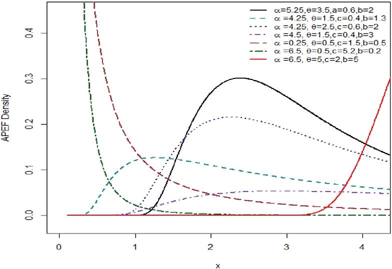
Figure 1 Plots of the APEF densities.

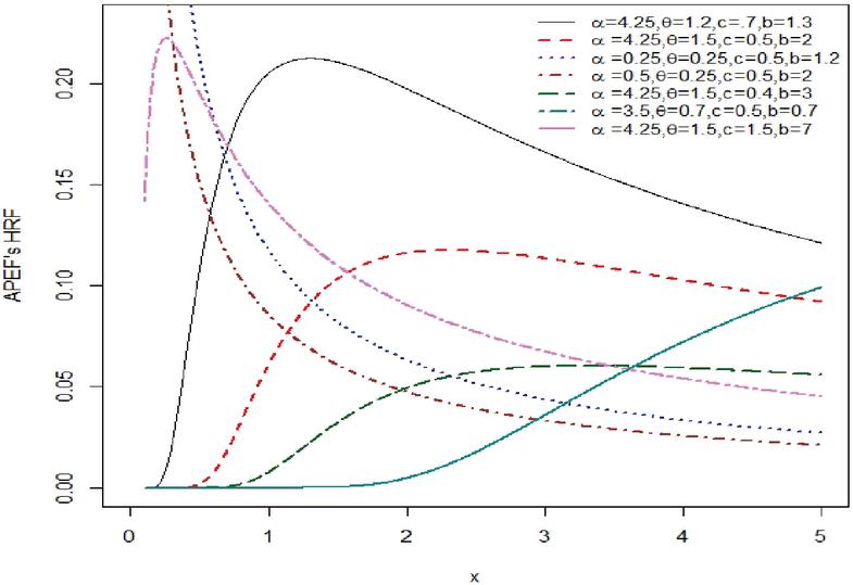
Figure 2 Plots of the APEF hazard rates.

Plots of the APEF density in Equation (6) and hazard rate in Equation (8) are displayed, respectively, in Figures 1 and 2. It is observed from Figure 1 the various shapes of APEF density function as it takes decreasing, increasing, and right-skewed shapes. Additionally, as demonstrated in Figure 2, the HRF of APEF can take several shapes, including monotonically decreasing, uni-modal, and reversed j-shape. Therefore, this illustrates APEF’s considerable versatility, making it ideal for a wide range of real-world applications.

2.1 Special Sub-Models

The APEF approaches several distributions such as the Fréchet, EF, inverse exponential (IE) [21], APT-Fréchet and APT-IE [11]. Table 1 shows the essential sub-models of APEF.

Table 1 Special sub-models of the APEF

$\alpha$	b	c	$\theta$	Resulting Distribution
$-$	$b$	$-$	$\theta$	Fréchet
$-$	$b$	$c$	$\theta$	EF
$-$	b	$-$	$-$	IE
$\alpha$	$b$	$-$	$\theta$	APF
$\alpha$	b	$-$	$-$	AP-IE

3 Important Expansion of the APEF Density

This section presents essential expansion of the APEF density to simplify the derivation of APEF structural properties. The exponential series representation for ${\alpha }^{-z}$ is expressed as

$${\alpha }^{-z}=\sum _{{\nu }_1=0}^{\mathrm{\infty }}\frac{{(-\log \alpha )}^{{\nu }_1}}{{\nu }_1!}{\left(z\right)}^{{\nu }_1}.$$

(9)

Therefore, employing Equation (9) to Equation (6) for $\alpha \ne 1$, the PDF of APEF will be

$f(x)$	$={\displaystyle \frac{\log \alpha }{\alpha -1}}\alpha b^{\theta }\theta c{x}^{-(\theta +1)}\exp \left\{-{\left({\displaystyle \frac{b}{x}}\right)}^{\theta }\right\}{\displaystyle \sum _{{\nu }_1=0}^{\mathrm{\infty }}}{\displaystyle \frac{{(-\log \alpha )}^{{\nu }_1}}{{\nu }_1!}}$
	$\mathrm{\hspace{1em}}\times {\left[1-\exp \left\{-{\left({\displaystyle \frac{b}{x}}\right)}^{\theta }\right\}\right]}^{c{\nu }_1+(c-1)}.$

Then, by employing the following binomial series expansion

$${(1-z)}^{a-1}=\sum _{{\nu }_2=0}^{\mathrm{\infty }}{(-1)}^{{\nu }_2}\left(\genfrac{}{}{0pt}{}{a-1}{{\nu }_2}\right){(z)}^{{\nu }_2},$$

(10)

the PDF will be

$f(x)$	$={\displaystyle \frac{\alpha b^{\theta }\theta c}{\alpha -1}}{x}^{-(\theta +1)}{\displaystyle \sum _{{\nu }_1,{\nu }_2=0}^{\mathrm{\infty }}}{\displaystyle \frac{{(\log \alpha )}^{{\nu }_1+1}}{{\nu }_1!}}{(-1)}^{{\nu }_1+{\nu }_2}$
	$\mathrm{\hspace{1em}}\times \left({\displaystyle \genfrac{}{}{0pt}{}{c(\nu 1+1)-1}{{\nu }_2}}\right){\left[\exp \left\{-{\left({\displaystyle \frac{b}{x}}\right)}^{\theta }\right\}\right]}^{{\nu }_2+1}.$

Then, the PDF of APEF can be reduced to

$$f(x)=b^{\theta }\theta \sum _{{\nu }_2=0}^{\mathrm{\infty }}{\eta }_{{\nu }_2}{x}^{-(\theta +1)}\exp \left\{-({\nu }_2+1){\left(\frac{b}{x}\right)}^{\theta }\right\},$$

(11)

where

$${\eta }_{{\nu }_2}=\frac{\alpha c}{\alpha -1}\sum _{{\nu }_1}^{\mathrm{\infty }}\frac{{(-1)}^{{\nu }_1+{\nu }_2}{(\log \alpha )}^{{\nu }_1+1}}{{\nu }_1!}\left(\genfrac{}{}{0pt}{}{c({\nu }_1+1)-1}{{\nu }_2}\right).$$

(12)

4 Mathematical Properties

The following mathematical features of the APEF are investigated:

4.1 Quantile and Median

The $p^{th}$ quantile of the APEF could be expressed in the following form

$$Q_p=\frac{b}{{\left[-log\left(1-{\left(1-\frac{\log (p(\alpha -1)+1)}{log\alpha }\right)}^{\frac{1}{c}}\right)\right]}^{\frac{1}{\theta }}}.$$

(13)

Then setting $p=0.5$ in Equation (13), the median of the APEF is

$$Med=Q_{0.5}=\frac{b}{{\left[-log\left(1-{\left(1-\frac{\log (0.5(\alpha +1))}{log\alpha }\right)}^{\frac{1}{c}}\right)\right]}^{\frac{1}{\theta }}}.$$

(14)

4.2 Moments, Moment Generating and Characteristics Functions

The $r^{th}$ moment is obtained from Equation (11) as

$\begin{array}{cc}\hfill {\mu }_r& =E\left(x^r\right)={\displaystyle {\int }_0^{\mathrm{\infty }}}{x}^r{f}_{APEF}(x)\mathit{d}x\hfill \\ & =b^{\theta }\theta {\displaystyle \sum _{{\nu }_2=0}^{\mathrm{\infty }}}{\eta }_{{\nu }_2}{\displaystyle {\int }_0^{\mathrm{\infty }}}{x}^r{x}^{-(\theta +1)}\exp \left\{-({\nu }_2+1){\left({\displaystyle \frac{b}{x}}\right)}^{\theta }\right\}\mathit{d}x.\hfill \end{array}$

Taking $g=({\nu }_2+1){\left(\frac{b}{x}\right)}^{\theta },dx=\frac{x^{(\theta +1)}dg}{-b^{\theta }\theta ({\nu }_2+1)}$ , limits will change from $\mathrm{\infty }$ to $0$, then after some simplification, we have

$$E(x^r)=\sum _{{\nu }_2=0}^{\mathrm{\infty }}{\eta }_{{\nu }_2}\frac{b^r}{{({\nu }_2+1)}^{(1-\frac{r}{\theta })}}{\int }_0^{\mathrm{\infty }}{g}^{-\frac{r}{\theta }}\exp \left(-g\right)\mathit{d}g.$$

The $r^{th}$ moment of the APEF is expressed as

$${\mu }_r=\sum _{{\nu }_2=0}^{\mathrm{\infty }}{\eta }_{{\nu }_1}\frac{b^r\mathrm{\Gamma }((1-\frac{r}{\theta })}{{({\nu }_2+1)}^{(1-\frac{r}{\theta })}},r<\theta ,$$

(15)

where ${\eta }_{{\nu }_2}$ is defined in Equation (12). Subsequently, the mean and variance can be obtained by substituting $r=1$ and $r=2$ in Equation (15), respectively.

Therefore, based on the $r^{th}$ moment in Equation (15) of APEF, the moment generating function (mgf) is expressed as

$$M_x(t)=E(e^{tx})=\sum _{r=0}^{\mathrm{\infty }}\frac{t^r}{r!}{\mu }_r.$$

(16)

Substituting Equation (15) in Equation (16), will have

$$M_x(t)=\sum _{r=0}^{\mathrm{\infty }}\sum _{{\nu }_2=0}^{\mathrm{\infty }}{\eta }_{{\nu }_2}\frac{t^r}{r!}\frac{b^r\mathrm{\Gamma }((1-\frac{r}{\theta })}{{({\nu }_2+1)}^{(1-\frac{r}{\theta })}},r<\theta ,$$

(17)

where ${\eta }_{{\nu }_2}$ is defined in Equation (12).

Similarly, the characteristics function of APEF is easily obtained as

$${\varphi }_x(t)=E(e^{tx})=\sum _{r=0}^{\mathrm{\infty }}\sum _{{\nu }_2=0}^{\mathrm{\infty }}{\eta }_{{\nu }_2}\frac{{(it)}^r}{r!}\frac{b^r\mathrm{\Gamma }((1-\frac{r}{\theta })}{{({\nu }_2+1)}^{(1-\frac{r}{\theta })}},r<\theta ,$$

(18)

where ${\eta }_{{\nu }_2}$ is defined in Equation (12).

4.3 Incomplete Moment

The incomplete moment is considered important for many applications in various fields. Therefore, the $r^{th}$ incomplete moment of APEF is derived using Equation (11) as

$\begin{array}{cc}\hfill {\xi }^r& ={\displaystyle {\int }_0^t}{x}^r{f}_{APEF}(x)\mathit{d}x\hfill \\ & =b^{\theta }\theta {\displaystyle \sum _{{\nu }_2=0}^{\mathrm{\infty }}}{\eta }_{{\nu }_2}{\displaystyle {\int }_0^t}{x}^{-(\theta +1)+r}\exp \left\{-({\nu }_2+1){\left({\displaystyle \frac{b}{x}}\right)}^{\theta }\right\}\mathit{d}x\hfill \end{array}$

Then after some simplification and using the incomplete gamma function given by

$${\mathrm{\Gamma }}^{*}(s,x)={\int }_x^{\mathrm{\infty }}{w}^{s-1}{e}^{-w}\mathit{d}w,$$

the APEF’s incomplete moment is expressed as

$${\xi }^r=\sum _{{\nu }_2=0}^{\mathrm{\infty }}{\eta }_{{\nu }_2}\frac{b^r{\mathrm{\Gamma }}^{*}(1-\frac{r}{\theta },({\nu }_2+1){\left(\frac{b}{x}\right)}^{\theta })}{{({\nu }_2+1)}^{(1-\frac{r}{\theta })}},r<\theta .$$

(19)

4.4 Mean Residual Life Function and Mean Waiting Time

If $X\sim APEF$, then the mean residual life function of $X$, $\mu (t)$, is defined as

$$\mu (t)=\frac{1}{S(t)}\left(E(t)-{\int }_0^{t}xf(x)\mathit{d}x\right)-t,$$

(20)

where

$\begin{array}{cc}\hfill {\displaystyle {\int }_0^t}xf(x)\mathit{d}x& ={\displaystyle {\int }_0^t}x{b}^{\theta }\theta {\displaystyle \sum _{{\nu }_2=0}^{\mathrm{\infty }}}{\eta }_{{\nu }_2}{x}^{-(\theta +1)}\exp \left\{-({\nu }_2+1){\left({\displaystyle \frac{b}{x}}\right)}^{\theta }\right\}dx.\hfill \\ & ={\displaystyle \sum _{{\nu }_2=0}^{\mathrm{\infty }}}{\eta }_{{\nu }_2}{\displaystyle \frac{b{\mathrm{\Gamma }}^{*}(1-\frac{1}{\theta },({\nu }_2+1){\left(\frac{b}{t}\right)}^{\theta })}{{({\nu }_2+1)}^{(1-\frac{1}{\theta })}}}.\hfill \end{array}$

(21)

Substituting Equation (7), Equation (15), and Equation (21) in Equation (20), then

$\mu (t)$

$={\displaystyle \frac{(\alpha -\mathrm{\hspace{0.17em}1})({\sum }_{{\nu }_2=0}^{\mathrm{\infty }}\frac{{\eta }_{{\nu }_2}b}{{({\nu }_2+1)}^{(1-\frac{1}{\theta })}}[\mathrm{\Gamma }(1-\frac{1}{\theta })-{\mathrm{\Gamma }}^{*}(1-\frac{1}{\theta },({\nu }_2+\mathrm{\hspace{0.17em}1}){(\frac{b}{t})}^{\theta })])}{\alpha (1-{\alpha }^{-{[1-\exp \{-{(\frac{b}{t})}^{\theta }\}]}^a})}}-t.$

(22)

Similarly, the mean waiting time is

$\begin{array}{cc}\hfill \overline{\mu }(t)& =t-{\displaystyle \frac{1}{F(t)}}{\displaystyle {\int }_0^t}xf(x)\mathit{d}x\hfill \\ & =t-{\displaystyle \frac{(\alpha -1)\left({\sum }_{{\nu }_2=0}^{\mathrm{\infty }}\frac{{\eta }_{{\nu }_2}b}{{({\nu }_2+1)}^{(1-\frac{1}{\theta })}}\left[{\mathrm{\Gamma }}^{*}(1-\frac{1}{\theta },({\nu }_2+1){\left(\frac{b}{t}\right)}^{\theta })\right]\right)}{{\alpha }^{1-{\left[1-\exp \left\{-{\left(\frac{b}{t}\right)}^{\theta }\right\}\right]}^a}}}.\hfill \end{array}$

4.5 Rényi Entropy

The Rényi entropy for a random variable $X$ denoted by $R{E}_x$ presents a variation measure of uncertainty and is takes the following form

$R{E}_x(\delta )={\displaystyle \frac{1}{1-\delta }}log\left({\displaystyle {\int }_{-\mathrm{\infty }}^{\mathrm{\infty }}}{\left[f(x)\right]}^{\delta }\mathit{d}x\right);\delta >0,\nu \ne 0.$

Then from Equation (6), will have

$\begin{array}{cc}\hfill {\left[f(x)\right]}^{\delta }& ={\left[{\displaystyle \frac{\log \alpha }{\alpha -1}}\right]}^{\delta }\hfill \\ & \times {\displaystyle \frac{{\left(\alpha b^{\theta }\theta c\right)}^{\delta }{x}^{-\delta (\theta +1)}\exp \left\{-\delta {\left(\frac{b}{x}\right)}^{\theta }\right\}{\left[1-\exp \left\{-{\left(\frac{b}{x}\right)}^{\theta }\right\}\right]}^{\delta (c-1)}}{{\alpha }^{\delta {\left[1-\exp \left\{-{\left(\frac{b}{x}\right)}^{\theta }\right\}\right]}^c}}}.\hfill \end{array}$

Applying Equation (9) to expand ${\alpha }^{-\delta {\left[1-\exp \left\{-{\left(\frac{b}{x}\right)}^{\theta }\right\}\right]}^a}$, then

$\begin{array}{cc}\hfill {\left[f(x)\right]}^{\delta }& ={\left[{\displaystyle \frac{\alpha b^{\theta }\theta c\log \alpha }{\alpha -1}}\right]}^{\delta }{x}^{-\delta (\theta +1)}\exp \left\{-\delta {\left({\displaystyle \frac{b}{x}}\right)}^{\theta }\right\}\hfill \\ & \times {\displaystyle \sum _{{\nu }_1=0}^{\mathrm{\infty }}}{\displaystyle \frac{{(-\log \alpha )}^{{\nu }_1}}{{\nu }_1!}}{[1-\exp \{-{\left({\displaystyle \frac{b}{x}}\right)}^{\theta }\}]}^{c({\nu }_1+\delta )-\delta }.\hfill \end{array}$

Additionally, using Equation (10)

${\left[f(x)\right]}^{\delta }$	$={\displaystyle \frac{{\left(\alpha b^{\theta }\theta c\right)}^{\delta }{x}^{-\delta (\theta +1)}}{{(\alpha -1)}^{\delta }}}{\displaystyle \sum _{{\nu }_1,{\nu }_2=0}^{\mathrm{\infty }}}{\displaystyle \frac{{(-1)}^{{\nu }_1+{\nu }_2}}{{\nu }_1!}}{\left(\log \alpha \right)}^{{\nu }_1+\delta }$
	$\mathrm{\hspace{1em}}\times \left({\displaystyle \genfrac{}{}{0pt}{}{c({\nu }_1+\delta )-\delta }{{\nu }_2}}\right)\left[\exp \left\{-({\nu }_2+\delta ){\left({\displaystyle \frac{b}{x}}\right)}^{\theta }\right\}\right].$

Therefore,

$R{E}_x(\delta )$	$={\displaystyle \frac{1}{1-\delta }}log$
	$\mathrm{\hspace{1em}}\times \left\{{(b^{\theta }\theta )}^{\delta }{\displaystyle \sum _{{\nu }_2=0}^{\mathrm{\infty }}}{\eta }_{{\nu }_2}^{*}{\displaystyle {\int }_0^{\mathrm{\infty }}}{x}^{-\delta (\theta +1)}\exp \left\{-({\nu }_2+\delta ){\left({\displaystyle \frac{b}{x}}\right)}^{\theta }\right\}\mathit{d}x\right\},$

where

$${\eta }_{{\nu }_2}^{*}=\frac{{(\alpha c)}^{\delta }}{{(\alpha -1)}^{\delta }}\sum _{{\nu }_1}^{\mathrm{\infty }}\frac{{(-1)}^{{\nu }_1+{\nu }_2}}{{\nu }_1!}\left(\genfrac{}{}{0pt}{}{c({\nu }_1+\delta )-\delta }{{\nu }_2}\right){(\log \alpha )}^{{\nu }_1+\delta }.$$

(24)

By assuming $u=({\nu }_2+\delta ){\left(\frac{b}{x}\right)}^{\theta }$, $R{E}_x$ for the APEF can be expressed as

$\begin{array}{c}\hfill R{E}_x(\delta )={\displaystyle \frac{1}{1-\delta }}log\left\{b^{1-\delta }{\theta }^{\delta -1}{\displaystyle \sum _{{\nu }_2=0}^{\mathrm{\infty }}}{\eta }_{{\nu }_2}^{*}{\displaystyle \frac{\mathrm{\Gamma }\left(\frac{\delta (\theta +1)-1}{\theta }\right)}{{({\nu }_2+\delta )}^{\frac{\delta (\theta +1)-1}{\theta }}}}\right\}.\end{array}$

(25)

4.6 Order Statistics

If a random sample $X_1,\mathrm{\dots },X_n$ is obtained from APEF in Equation (11), then $X_{k:n}$ denotes the $k^{th}$ order statistics with the following PDF

$$f_{k:n}(x)=\frac{n!}{(k-1)!(n-k)!}f(x)F{(x)}^{k-1}{[1-F(x)]}^{n-k}.$$

(26)

Inserting Equations (6) and (5) into Equation (26), will have

$f_{k:n}(x)$	$={\displaystyle \frac{n!{(-1)}^{k-1}f(x)}{(k-1)!(n-k)!{(\alpha -1)}^{n-1}}}{\left(1-{\alpha }^{1-{\left[1-\exp \left\{-{\left(\frac{b}{x}\right)}^{\theta }\right\}\right]}^c}\right)}^{k-1}$
	$\mathrm{\hspace{1em}}\times {\left(\alpha -{\alpha }^{1-{\left[1-\exp \left\{-{\left(\frac{b}{x}\right)}^{\theta }\right\}\right]}^c}\right)}^{n-k}.$

Applying the binomial theorem

${(x-z)}^m={\displaystyle \sum _{y=0}^m}{(-1)}^y\left({\displaystyle \genfrac{}{}{0pt}{}{m}{y}}\right)x^{m-y}{z}^y.$

Then, $f_{k:n}(x)$ can be expressed as

$\begin{array}{cc}\hfill f_{k:n}(x)& ={\displaystyle \frac{n!b^{\theta }\theta c\log \alpha }{(k-1)!(n-k)!{(\alpha -1)}^n}}{x}^{-(\theta +1)}\hfill \\ & \times \exp \left\{-{\left({\displaystyle \frac{b}{x}}\right)}^{\theta }\right\}{\left[1-\exp \left\{-{\left({\displaystyle \frac{b}{x}}\right)}^{\theta }\right\}\right]}^{c-1}\hfill \\ & \times {\displaystyle \sum _{{\lambda }_1=0}^{k-1}}{\displaystyle \sum _{\lambda =0}^{n-k}}\left({\displaystyle \genfrac{}{}{0pt}{}{k-1}{{\lambda }_1}}\right)\left({\displaystyle \genfrac{}{}{0pt}{}{n-k}{{\lambda }_2}}\right){\displaystyle \frac{{(-1)}^{k+{\lambda }_1+{\lambda }_2-1}{\alpha }^{n-k+{\lambda }_1+1}}{{\alpha }^{({\lambda }_1+{\lambda }_2+1){\left[1-\exp \left\{-{\left(\frac{b}{x}\right)}^{\theta }\right\}\right]}^c}}}.\hfill \end{array}$

(27)

5 Estimation

We assume that $x_1,x_2,\mathrm{\dots },x_n$ is a random sample from the APEF. Then, the log-likelihood ($\mathrm{\ell }$) for $\mathrm{\Theta }=(\alpha ,b,\theta ,c)$ is

$\begin{array}{cc}\hfill \mathrm{\ell }& =n\log \left({\displaystyle \frac{\log \left(\alpha \right)}{\alpha -1}}\right)+n\log \left(\alpha b^{\theta }\theta c\right)-(\theta +1){\displaystyle \sum _{i=1}^n}\log (x_i)-{\displaystyle \sum _{i=1}^n}{\left({\displaystyle \frac{b}{x_i}}\right)}^{\theta }\hfill \\ & +\left(c-1\right){\displaystyle \sum _{i=1}^n}\log \left(1-\exp \left\{-{\left({\displaystyle \frac{b}{x_i}}\right)}^{\theta }\right\}\right)\hfill \\ & -\log \alpha {\displaystyle \sum _{i=1}^n}{\left(1-\exp \left\{-{\left({\displaystyle \frac{b}{x_i}}\right)}^{\theta }\right\}\right)}^c.\hfill \end{array}$

(28)

Then, the likelihood equations are as follows:

${\displaystyle \frac{\partial \mathrm{\ell }}{\partial \alpha }}={\displaystyle \frac{n\left(\frac{\alpha -1}{\alpha }-\log \alpha \right)}{\left(\alpha -1\right)\log \alpha }}+{\displaystyle \frac{n}{\alpha }}-{\displaystyle \frac{{\sum }_{i=1}^n{\left(1-\exp \left\{-{\left(\frac{b}{x_i}\right)}^{\theta }\right\}\right)}^c}{\alpha }},$

$\begin{array}{cc}\hfill {\displaystyle \frac{\partial \mathrm{\ell }}{\partial b}}& ={\displaystyle \frac{n\theta }{b}}-{\displaystyle \sum _{i=1}^n}{\displaystyle \frac{\theta {\left(\frac{b}{x_i}\right)}^{\theta -1}}{x_i}}+\left(c-1\right)\theta {\displaystyle \sum _{i=1}^n}{\displaystyle \frac{{\left(\frac{b}{x_i}\right)}^{\theta -1}\exp \left\{-{\left(\frac{b}{x_i}\right)}^{\theta }\right\}}{x\left(1-\exp \left\{-{\left(\frac{b}{x_i}\right)}^{\theta }\right\}\right)}}\hfill \\ & -\theta c{\displaystyle \sum _{i=1}^n}{\displaystyle \frac{{\left(\frac{b}{x_i}\right)}^{\theta -1}\exp \left\{-{\left(\frac{b}{x_i}\right)}^{\theta }\right\}{\left(1-\exp \left\{-{\left(\frac{b}{x_i}\right)}^{\theta }\right\}\right)}^{c-1}}{x_i}}\log \alpha ,\hfill \end{array}$

$\begin{array}{cc}\hfill {\displaystyle \frac{\partial \mathrm{\ell }}{\partial \theta }}& ={\displaystyle \frac{n\left(\theta b^{\theta }\log \left(b\right)+b^{\theta }\right)}{\theta b^{\theta }}}-{\displaystyle \sum _{i=1}^n}{\left({\displaystyle \frac{b}{x_i}}\right)}^{\theta }\log \left({\displaystyle \frac{b}{x_i}}\right)-{\displaystyle \sum _{i=1}^n}\log \left(x_i\right)\hfill \\ & +\left(c-1\right){\displaystyle \sum _{i=1}^n}{\left({\displaystyle \frac{b}{x_i}}\right)}^{\theta }\log \left({\displaystyle \frac{b}{x_i}}\right){\displaystyle \frac{\exp \left\{-{\left(\frac{b}{x_i}\right)}^{\theta }\right\}}{\left(1-\exp \left\{-{\left(\frac{b}{x_i}\right)}^{\theta }\right\}\right)}}\hfill \\ & -c{\displaystyle \sum _{i=1}^n}{\left({\displaystyle \frac{b}{x_i}}\right)}^{\theta }\log \left({\displaystyle \frac{b}{x_i}}\right){\left(1-\exp \left\{-{\left({\displaystyle \frac{b}{x_i}}\right)}^{\theta }\right\}\right)}^{c-1}\hfill \\ & \times \exp \left\{-{\left({\displaystyle \frac{b}{x_i}}\right)}^{\theta }\right\}\log \alpha ,\hfill \end{array}$

and

${\displaystyle \frac{\partial \mathrm{\ell }}{\partial c}}$	$={\displaystyle \frac{n}{c}}+{\displaystyle \sum _{i=1}^n}\log \left(1-\exp \left\{-{\left({\displaystyle \frac{b}{x_i}}\right)}^{\theta }\right\}\right)$
	$\mathrm{\hspace{1em}}-{\displaystyle \sum _{i=1}^n}{\left(1-\exp \left\{-{\left({\displaystyle \frac{b}{x_i}}\right)}^{\theta }\right\}\right)}^c$
	$\mathrm{\hspace{1em}}\times \log \left(1-\exp \left\{-{\left({\displaystyle \frac{b}{x_i}}\right)}^{\theta }\right\}\right)\log \alpha .$

The ML estimates of $\alpha ,b,\theta$ and $c$ is obtained by solving the above equations simultaneously or by directly maximizing Equation (28) by non-linear optimization approach.

6 Numerical Studies

In this numerical study, 1000 samples with size 25, 50, 100, 200 and 500 are randomly generated from the APEF for two combinations of parameter values as follows:

• Combination1:  $\alpha =0.7,b=1.9,\theta =5.5,c=1.2)$,

• Combination2:  $\alpha =1.5,b=3.9,\theta =6,c=0.2)$.

The ML estimates and mean square errors (MSEs),

$${\widehat{MSE}}_b=\frac{1}{n}\sum _{i=1}^n{({\widehat{\mathrm{\Theta }}}_i-\mathrm{\Theta })}^2,$$

are calculated to assess the performance of ML estimators.

Table 2 ML estimates and MSE for two combinations of parameter’ values

		First Combination		Second Combination
Sample size	Par.	Estimate	MSE	Estimate	MSE
$n=25$	$\alpha$	0.8855	0.7785	1.5512	0.9403
	$b$	1.3698	0.7105	4.0663	0.4758
	$\theta$	5.5369	0.7197	6.1416	0.7804
	$c$	1.3698	0.7105	0.2170	0.1958
$n=50$	$\alpha$	0.8098	0.6104	1.5198	0.6157
	$b$	1.9175	0.0745	3.9867	0.2666
	$\theta$	5.5100	0.5641	6.0638	0.4366
	$c$	1.2557	0.4910	0.2049	0.0491
$n=100$	$\alpha$	0.7514	0.4504	1.5577	0.4427
	$b$	1.9146	0.0535	3.9334	0.1737
	$\theta$	5.4751	0.3622	6.0300	0.3126
	$c$	1.2221	0.3288	0.2034	0.0314
$n=200$	$\alpha$	0.7528	0.3984	1.4538	0.1859
	$b$	1.2031	0.1489	3.8653	0.0792
	$\theta$	5.4804	0.1802	6.1625	0.2228
	$c$	1.2031	0.1489	0.1881	0.0199
$n=500$	$\alpha$	0.7101	0.2521	1.4603	0.0450
	$b$	1.9066	0.0496	3.8268	0.0764
	$\theta$	5.5063	0.3433	6.1761	0.2017
	$c$	1.2082	0.2393	0.1824	0.0182

Table 2 reports the simulation results. The results revealed that the ML technique performs effectively as the parameter estimates get closer to their true values. Additionally, the MSEs decrease as the sample size increases for both parameter combinations.

7 Applications

In this section, the APEF is utilized to statistically assess six well-known data sets. In particular, the fit of APEF for each of the five data sets is compared with the fits of some of its sub-models and other competitive generalization of the EF and Fréchet distributions. The CDFs of these distributions are, respectively, as follows:

• APF:

$$F(x;b,\theta )=\frac{{\alpha }^{\exp \left\{-{\left(\frac{b}{x}\right)}^{\theta }\right\}}-1}{\alpha -1},\alpha \ne 1;$$

• TEF:

$F(x;\lambda ,b,\theta ,c)$	$=\left[1-{\left(1-\exp \left\{-{\left({\displaystyle \frac{b}{x}}\right)}^{\theta }\right\}\right)}^c\right]$
	$\mathrm{\hspace{1em}}\times \left[1+\lambda {\left(1-\exp \left\{-{\left({\displaystyle \frac{b}{x}}\right)}^{\theta }\right\}\right)}^c\right];$

• Marshall-Olkin exponentiated Fréchet (MO-EF):

$$F(x;\delta ,b,\theta )=1-\frac{\delta \left[1-\exp \left\{-{\left(\frac{b}{x}\right)}^{\theta }\right\}\right]}{\left[1-(1-\delta )\left(1-\exp \left\{-{\left(\frac{b}{x}\right)}^{\theta }\right\}\right)\right]};$$

• MO-EF:

$$F(x;\delta ,b,\theta ,c)=1-\frac{\delta {\left[1-\exp \left\{-{\left(\frac{b}{x}\right)}^{\theta }\right\}\right]}^c}{\left[1-(1-\delta ){\left(1-\exp \left\{-{\left(\frac{b}{x}\right)}^{\theta }\right\}\right)}^c\right]};$$

for $x>0;\alpha ,b,\theta ,c,\delta >0$ and $|\lambda |\le 1$.

The following goodness-of-fit (GOF) statistics are used to evaluate APEF’s performance compared to other models: Akaike Information Criterion (AIC), corrected AIC (CAIC), Kramér-von Mises (W*), Anderson-Darling (A*), Kolmogorov-Smirnov (KS) and P-value statistics. The model with the shortest values of these statistics, as well as the highest P-value for the KS test, is the best. The calculations are carried out using the package fitdistrplus in the R software [40]. In addition, the fitted CDFs and PDFs of APEF and other competitive models are plotted and compared.

First data set: The first data set were taken from [39], which report the highest annual flood flows of the North Saskachevan River near Edmonton in units of 1000 cubic feet per second for a 48-year period. The data are illustrated Table 8 in the Appendix.

Second data set: The data was studied by [25] and illustrate the Mathematics grades for 48 slow-pace students in the year 2013, see Table 9 in the Appendix.

Third data set: This data present drought mortality rate and are recently studied by [3, 4]. The data report Canada COVID-19 data from 10 April to 15 May 2020 for 36 days, The data are illustrated Table 10 in the Appendix.

Fourth data set: This data corresponds to the remission months of $128$ patients suffering from bladder cancer, see [2], see Table 11 in the Appendix.

Fifth data set: This data obtained from [41] which report the survival times of 121 breast cancer patients in the period between 1929 to 1938, see Table 12 in the Appendix.

Table 3 ML estimation and associated GOF statistics for data 1

Distribution	APEF	APF	EF	TEF	MO-F	MO-EF
Estimates	$\widehat{\alpha }=$ 16.132	$\widehat{\alpha }=$ 122.295	$\widehat{c}=$ 0.099	$\widehat{\lambda }=$ 0.521	$\widehat{\delta }=$ 16.671	$\widehat{\delta }=13.789$
	$\widehat{\theta }=$ 15.444	$\widehat{\theta }=$ 4.633	$\widehat{b}=$ 21.673	$\widehat{\theta }=$ 0.836	$\widehat{\theta }=$ 3.407	$\widehat{c}=0.164$
	$\widehat{c}=$ 0.142	$\widehat{b}=$ 26.750	$\widehat{\theta }=$ 13.906	$\widehat{c}=$ 8.109	$\widehat{b}=$ 18.797	$\widehat{b}=$ 10.795
	$\widehat{b}=$ 20.447			$\widehat{b}=$ 154.094		$\widehat{\theta }=$ 13.155
AIC	437.416	466.474	443.753	441.738	440.474	455.488
CAIC	441.159	469.281	446.560	445.480	442.878	459.2305
W*	0.0243	0.4947	0.2970	0.0581	0.0774	0.4056
AD*	0.1652	5.6861	1.5364	0.3924	0.5075	2.4708
KS	0.0647	0.2018	0.1450	0.0860	0.0918	0.1856
P-value	0.9878	0.0401	0.2644	0.8693	0.9075	0.0731

Table 4 ML estimation and associated GOF statistics for data 2

Distribution	APEF	APF	EF	TEF	MO-F	MO-EF
Estimates	$\widehat{\alpha }=$ 4.5076	$\widehat{\alpha }=$ 64.798	$\widehat{c}=$ 2.044	$\widehat{\lambda }=$ -0.723	$\widehat{\delta }=$ 2.530	$\widehat{\delta }=64.798$
	$\widehat{\theta }=$ 0.628	$\widehat{\theta }=$ 1.727	$\widehat{b}=$ 22.760	$\widehat{\theta }=$ 1.591	$\widehat{\theta }=$ 1.739	$\widehat{c}=0.367$
	$\widehat{c}=$ 7.501	$\widehat{b}=$ 8.078	$\widehat{\theta }=$ 1.049	$\widehat{c}=$ 0.945	$\widehat{b}=$ 10.862	$\widehat{b}=$ 3.474
	$\widehat{b}=$ 60.877			$\widehat{b}=$ 10.942		$\widehat{\theta }=$ 6.412
AIC	401.1407	403.2002	403.2120	408.3653	404.8800	401.4828
CAIC	404.8831	406.007	406.0188	412.1077	407.6868	405.2252
W*	0.0348	0.0639	0.1197	0.0748	0.0683	0.0361
AD*	0.2537	0.5360	0.7189	0.8012	0.7112	0.2805
KS	0.0620	0.0911	0.1195	0.0795	0.0753	0.0637
P-value	0.9926	0.8201	0.4988	0.9214	0.9003	0.9899

Table 5 ML estimation and associated GOF statistics for data 3

Distribution	APEF	APF	EF	TEF	MO-F	MO-EF
Estimates	$\widehat{\alpha }=$ 25.4200	$\widehat{\alpha }=$ 22.100	$\widehat{c}=$ 1.964	$\widehat{\lambda }=$ 0.643	$\widehat{\delta }=$ 8.612	$\widehat{\delta }=5.699$
	$\widehat{\theta }=$ 1.315	$\widehat{\theta }=$ 3.970	$\widehat{b}=$ 3.303	$\widehat{\theta }=$ 1.166	$\widehat{\theta }=$ 6.915	$\widehat{c}=6.915$
	$\widehat{c}=$ 9.729	$\widehat{b}=$ 2.142	$\widehat{\theta }=$ 2.446	$\widehat{c}=$ 15.757	$\widehat{b}=$ 1.938	$\widehat{b}=$ 3.914
	$\widehat{b}=$ 5.146			$\widehat{b}=$ 7.542		$\widehat{\theta }=$ 1.625
AIC	102.524	106.0610	107.1282	103.2653	103.8935	102.6079
CAIC	105.691	108.4363	109.5034	106.4324	106.2688	105.775
W*	0.0589	0.1661	0.1925	0.0719	0.1715	0.0715
AD*	0.3665	1.0178	1.1300	0.4381	0.9423	0.4211
KS	0.0985	0.1412	0.1560	0.1029	0.1503	0.1121
P-value	0.8757	0.4689	0.3448	0.8401	0.3901	0.7553

Table 6 ML estimation and associated GOF statistics for data 4

Distribution	APEF	APF	EF	TEF	MO-F	MO-EF
Estimates	$\widehat{\alpha }=$ 60.757	$\widehat{\alpha }=$ 18.940	$\widehat{c}=$ 4.320	$\widehat{\lambda }=$ -0.826	$\widehat{\delta }=$ 17.497	$\widehat{\delta }=12.227$
	$\widehat{\theta }=$ 0.245	$\widehat{\theta }=$ 0.939	$\widehat{b}=$ 18.748	$\widehat{\theta }=$ 0.451	$\widehat{\theta }=$ 1.233	$\widehat{c}=5.715$
	$\widehat{c}=$ 24.644	$\widehat{b}=$ 1.204	$\widehat{\theta }=$ 0.487	$\widehat{c}=$ 4.726	$\widehat{b}=$ 0.516	$\widehat{b}=$ 6.319
	$\widehat{b}=$ 328.959			$\widehat{b}=$ 14.554		$\widehat{\theta }=$ 0.456
AIC	827.8689	871.4901	851.3876	842.6851	855.0750	829.7104
CAIC	833.5729	875.7681	855.6656	848.3892	859.3531	835.4145
W*	0.0145	0.6410	0.5596	0.1750	0.4918	0.0315
AD*	0.1312	4.1151	2.9321	1.1764	3.0411	0.2402
KS	0.0351	0.1153	0.1185	0.0718	0.1116	0.0451
P-value	0.9974	0.0665	0.0550	0.5232	0.0821	0.9563

Table 7 ML estimation and associated GOF statistics for data 5

Distribution	APEF	APF	EF	TEF	MO-F	MO-EF
Estimates	$\widehat{\alpha }=$ 658.747	$\widehat{\alpha }=$ 20.417	$\widehat{c}=$ 2.855	$\widehat{\lambda }=$ -0.906	$\widehat{\delta }=$ 22.815	$\widehat{\delta }=25.439$
	$\widehat{\theta }=$ 0.253	$\widehat{\theta }=$ 0.833	$\widehat{b}=$ 59.676	$\widehat{\theta }=$ 0.611	$\widehat{\theta }=$ 1.155	$\widehat{c}=$4.640
	$\widehat{c}=$ 19.119	$\widehat{b}=$ 5.127	$\widehat{\theta }=$ 0.521	$\widehat{c}=$ 1.808	$\widehat{b}=$ 1.904	$\widehat{b}=$ 15.629
	$\widehat{b}=$ 764.733			$\widehat{b}=$ 17.141		$\widehat{\theta }=$ 0.502
AIC	1181.749	1252.361	1235.402	1234.778	1227.987	1183.347
CAIC	1187.34	1256.554	1239.596	1240.37	1232.181	1188.939
W*	0.1672	1.3575	1.2226	0.9502	1.0044	0.1930
AD*	1.1800	8.2502	6.7873	5.7262	6.2280	1.2830
KS	0.1086	0.1724	0.1748	0.1506	0.1446	0.1111
P-value	0.1147	0.0014	0.0012	0.0082	0.0126	0.1007

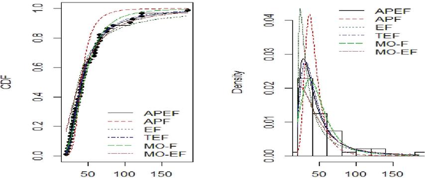
Figure 3 Estimated PDFs and CDFs of APEF, APF, EF, TEF, MO-F, and MO-EF distributions for data 1.

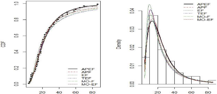
Figure 4 Estimated PDFs and CDFs of APEF, APF, EF, TEF, MO-F, and MO-EF distributions for data 2.

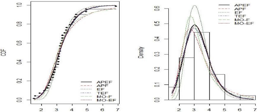
Figure 5 Estimated PDFs and CDFs of APEF, APF, EF, TEF, MO-F, and MO-EF distributions for data 3.

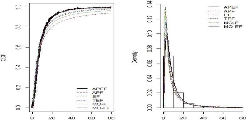
Figure 6 Estimated PDFs and CDFs of APEF, APF, EF, TEF, MO-F, and MO-EF distributions for data 4.

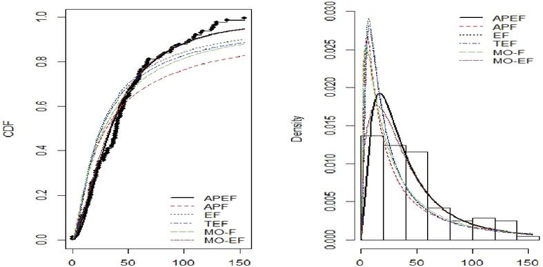
Figure 7 Estimated PDFs and CDFs of APEF, APF, EF, TEF, MO-F, and MO-EF distributions for data 5.

Tables 3–7 report the ML estimation and associated GOF statistics for each model. It can be observed that the GOF statistics are lower for APEF compared to other competitive models, and hence it provides a better fit for all five data sets. Moreover, the promising performance of APEF can be visually seen in Figures 3–7 as its estimated fits for the five data sets are closer to their empirical CDFs and PDFs.

8 Concluding Remarks

This article proposed a new generalization of EF distribution using APT named Alpha power exponentiated Fréchet distribution. The APEF provides high flexibility, especially for modeling skewed data in different fields. Explicit expressions of various mathematical properties of APEF such as quantile, median, moments, incomplete moments, mean residual life, order statistics, and entropy are derived. The performance of APEF is examined via simulation and Five real-life applications in different fields, which demonstrate its usefulness and great flexibility. Application results indicate that the APEF distribution consistently provides appropriate fit and outperformed other extended forms of the exponentiated Fréchet and Fréchet distributions.

Acknowledgement

The authors would like to thank to the editor and all of the referees for their thoughtful comments, which have helped to improve the manuscript.

Appendix

Table 8 List of Data set I

19.885	20.940	21.820	23.700	24.888	25.460	25.760	26.720	27.500	28.100
28.600	30.200	30.380	31.500	32.600	32.680	34.400	35.347	35.700	38.100
39.020	39.200	40.000	40.400	40.400	42.250	44.020	44.730	44.900	46.300
50.330	51.442	57.220	58.700	58.800	61.200	61.740	65.440	65.597	66.000
74.100	75.800	84.100	106.600	109.700	121.970	121.970	185.560

Table 9 List of Data set II

29	25	50	15	13	27	15	18	7	7	8	19	12	18	5	21	15
86	21	15	14	39	15	14	70	44	6	23	58	19	50	23	11	6
34	18	28	34	12	37	4	60	20	23	40	65	19	31

Table 10 List of Data set III

3.1091	3.3825	3.1444	3.2135	2.4946	3.5146	4.9274	3.3769	6.8686	3.0914	4.9378
3.1091	3.2823	3.8594	4.0480	4.1685	3.6426	3.2110	2.8636	3.2218	2.9078	3.6346
2.7957	4.2781	4.2202	1.5157	2.6029	3.3592	2.8349	3.1348	2.5261	1.5806	2.7704
2.1901	2.4141	1.9048

Table 11 List of Data set IV

0.08	2.09	3.48	4.87	6.94	8.66	13.11	23.63	0.20	2.23	3.52	4.98	6.97
9.02	13.29	0.40	2.26	3.57	5.06	7.09	9.22	13.80	25.74	0.50	2.46	3.64
5.09	7.26	9.47	14.24	25.82	0.51	2.54	3.70	5.17	7.28	9.74	14.76	26.31
0.81	2.62	3.82	5.32	7.32	10.06	14.77	32.15	2.64	3.88	5.32	7.39	10.34
14.83	34.26	0.90	2.69	4.18	5.34	7.59	10.66	15.96	36.66	1.05	2.69	4.23
5.41	7.62	10.75	16.62	43.01	1.19	2.75	4.26	5.41	7.63	17.12	46.12	1.26
2.83	4.33	5.49	7.66	11.25	17.14	79.05	1.35	2.87	5.62	7.87	11.64	17.36
1.40	3.02	4.34	5.71	7.93	11.79	18.10	1.46	4.40	5.85	8.26	11.98	19.13
1.76	3.25	4.50	6.25	8.37	12.02	2.02	3.31	4.51	6.54	8.53	12.03	20.28
2.02	3.36	6.76	12.07	21.73	2.07	3.36	6.93	8.65	12.63	22.69

Table 12 List of Data set V

0.3	0.3	4.0	5.0	5.6	6.2	6.3	6.6	6.8	7.4	7.5	8.4	8.4
10.3	11.0	11.8	12.2	12.3	13.5	14.4	14.4	14.8	15.5	15.7	16.2	16.3
16.5	16.8	17.2	17.3	17.5	17.9	19.8	20.4	20.9	21.0	21.0	21.1	23.0
23.4	23.6	24.0	24.0	27.9	28.2	29.1	30.0	31.0	31.0	32.0	35.0	35.0
37.0	37.0	37.0	38.0	38.0	38.0	39.0	39.0	40.0	40.0	40.0	41.0	41.0
41.0	42.0	43.0	43.0	43.0	44.0	45.0	45.0	46.0	46.0	47.0	48.0	49.0
51.0	51.0	51.0	52.0	54.0	55.0	56.0	57.0	58.0	59.0	60.0	60.0	60.0
61.0	62.0	65.0	65.0	67.0	67.0	68.0	69.0	78.0	80.0	83.0	88.0	89.0
90.0	93.0	96.0	103.0	105.0	109.0	109.0	111.0	115.0	117.0	125.0	126.0	127.0
129.0	129.0	139.0	154.0

References

[1] Afify, A., Yousof, H., Cordeiro, G., Ortega, E. & Nofal, Z. The Weibull Fréchet distribution and its applications. Journal of Applied Statistics. 43, 2608–2626, 2016.

[2] Al-Marzouki, S., Jamal, F., Chesneau, C. & Elgarhy, M. Type II Topp Leone power Lomax distribution with applications. Mathematics. 8(4), 2020.

[3] Almetwally, E., Alharbi, R., Alnagar, D. & Hafez, E. A New Inverted Topp-Leone Distribution: Applications to the COVID-19 Mortality Rate in Two Different Countries. Axioms. 10(25), 2021.

[4] Alotaibi, R., Khalifa, M., Baharith, L., Dey, S. & Rezk, H. The Mixture of the Marshall–Olkin Extended Weibull Distribution under Type-II Censoring and Different Loss Functions. Mathematical Problems in Engineering, 2021.

[5] Alzaatreh, A. & Ghosh, I. On the Weibull-X family of distributions. Journal of Statistical Theory and Applications. 14, 169–183, 2015.

[6] Alzaatreh, A., Lee, C. & Famoye, F. A new method for generating families of continuous distributions. Metron. 71, 63–79, 2013.

[7] Baharith, L. & Aljuhani, W. New Method for Generating New Families of Distributions. Symmetry. 13(4), pp. 726, 2021.

[8] Baharith, L. & Alamoudi, H. The Exponentiated Fréchet Generator of Distributions with Applications. Symmetry. 13(4), pp. 572, 2021.

[9] Barreto-Souza, W., Cordeiro, G. & Simas, A. Some results for beta Fréchet distribution. Communications in Statistics-Theory and Methods. 40, 798–811, 2011.

[10] Bourguignon, M., Silva, R. & Cordeiro, G. The Weibull-G family of probability distributions. Journal of Data Science. 12, 53–68, 2014.

[11] Ceren, Ü., Cakmakyapan, S. & Gamze, Ö. Alpha power inverted exponential distribution: Properties and application. Gazi University Journal of Science. 31, 954–965, 2018.

[12] Coles, S., Bawa, J., Trenner, L. & Dorazio, P. An introduction to statistical modeling of extreme values. Springer, 2001.

[13] Cordeiro, G. & Castro, M. A new family of generalized distributions. Journal of Statistical Computation and Simulation. 81, 883–898, 2011.

[14] Dey, S., Ghosh, I. & Kumar, D. Alpha-power transformed Lindley distribution: properties and associated inference with application to earthquake data. Annals of Data Science. 6, 623–650, 2019.

[15] Eghwerido, J. The alpha power Weibull Frechet distribution: properties and applications. Turkish Journal of Science. 5, 170–185, 2020.

[16] Eghwerido, J., Nzei, L. & Agu, F. The alpha power Gompertz distribution: characterization, properties, and applications. Sankhya A. 1–27, 2020.

[17] Elbatal, I., Asha, G. & Raja, A. transmuted exponentiated Fréchet distribution: properties and applications. Journal of Statistics Applications & Probability. 3, pp. 379, 2014.

[18] Eugene, N., Lee, C. & Famoye, F. Beta-normal distribution and its applications. Communications in Statistics-Theory and Methods. 31, 497–512, 2002.

[19] Haq, M. & Elgarhy, M. The odd Fréchet-G family of probability distributions. Journal of Statistics Applications & Probability. 7, 189–203, 2018.

[20] Ihtisham, S., Khalil, A., Manzoor, S., Khan, S. & Ali, A. Alpha-Power Pareto distribution: Its properties and applications. PloS One. 14, 6:e0218027, 2019.

[21] Keller, A., Kamath, A. & Perera, U. Reliability analysis of CNC machine tools. Reliability Engineering. 3, 449–473 , 1982.

[22] Klakattawi, H. & Aljuhani, W. A New Technique for Generating Distributions Based on a Combination of Two Techniques: Alpha Power Transformation and Exponentiated TX Distributions Family. Symmetry. 13(3), pp. 412, 2021.

[23] Kotz, S. & Nadarajah, S. Extreme value distributions: theory and applications. World Scientific, 2000.

[24] Krishna, E., Jose, K., Alice, T. & Ristić, M. The Marshall-Olkin Fréchet distribution. Communications in Statistics-Theory and Methods. 42, 4091–4107, 2013.

[25] Linhart, H. & Zucchini, W. Model selection. John Wiley & Sons, 1986.

[26] Mahdavi, A. & Kundu, D. A new method for generating distributions with an application to exponential distribution. Communications in Statistics-Theory and Methods. 46, 6543–6557, 2017.

[27] Mead, M. A note on Kumaraswamy Fréchet distribution. Australia. 8, pp. 294–300, 2014.

[28] Nadarajah, S. & Kotz, S. The exponentiated Fréchet distribution. Interstat Electronic Journal. 14, pp. 1–7 , 2003.

[29] Nadarajah, S. & Kotz, S. The exponentiated type distributions. Acta Applicandae Mathematica. 92, 97–111, 2006.

[30] Nasiru, S. Extended odd Fréchet-G family of distributions. Journal of Probability and Statistics, 2018.

[31] Nasiru, S., Mwita, P. & Ngesa, O. Alpha power transformed Frechet distribution. Applied Mathematics & Information Sciences. 13: 129–141, 2019.

[32] Nassar, M., Alzaatreh, A., Mead, M. & Abo-Kasem, O. Alpha power Weibull distribution: Properties and applications. Communications in Statistics-Theory and Methods. 46, 10236–10252, 2017.

[33] Nassar, M., Kumar, D., Dey, S., Cordeiro, G. & Afify, A. The Marshall–Olkin alpha power family of distributions with applications. Journal of Computational And Applied Mathematics. pp. 351, 41–53, 2019.

[34] Reyad, H., Korkmaz, M., Afify, A., Hamedani, G. & Othman, S. The Fréchet Topp Leone-G family of distributions: Properties, characterizations and applications. Annals Of Data Science. 8(2), 345–366, 2021.

[35] Pillai, J. & Moolath, G. A New Generalization of the Fréchet Distribution: Properties and Application. Statistica. 79, 267–289, 2019.

[36] Riffi, M., Ansari, S. & Hamdan, M. A generalized transmuted Frechet distribution. J. Stat. Appl. Pro. 7, 1–10, 2019.

[37] Silva, R., Andrade, T., Maciel, D., Campos, R. & Cordeiro, G. A new lifetime model: The gamma extended Fréchet distribution. Journal of Statistical Theory and Applications. 12, 39–54, 2013.

[38] Tahir, M., Cordeiro, G., Alizadeh, M., Mansoor, M., Zubair, M. & Hamedani, G. The odd generalized exponential family of distributions with applications. Journal of Statistical Distributions and Applications. 2(1), 2015.

[39] Tahir, M., Hussain, M., Cordeiro, G., El-Morshedy, M. & Eliwa, M. A new Kumaraswamy generalized family of distributions with properties, applications, and bivariate extension. Mathematics. 8(11), pp. 1989, 2020

[40] Team, R. & Others R: A language and environment for statistical computing. Vienna, Austria, 2013.

[41] Yang, Y., Tian, W. & Tong, T. Generalized Mixtures of Exponential Distribution and Associated Inference. Mathematics. 9(12), pp. 1371, 2021.

[42] ZeinEldin, R., Haq, M., Hashmi, S. & Elsehety, M. Alpha power transformed inverse Lomax distribution with different methods of estimation and applications. Complexity, 2020.

Biography

Lamya A. Baharith is currently working as a Associate Professor at Department of Statistics, King Abdulaziz University, Jeddah, Saudi Arabia. She has contributed to various fields of Statistics through several research publications in different national and international journals of repute. She has also successfully completed some research projects in the field of Statistics.

Journal of Reliability and Statistical Studies, Vol. 15, Issue 1 (2022), 129–152.
doi: 10.13052/jrss0974-8024.1516
© 2022 River Publishers