Bayesian Estimation for the Two Log-Logistic Models Under Joint Type II Censoring Schemes

Ranjita Pandey and Pulkit Srivastava^*

Department of Statistics, University of Delhi, Delhi, India
E-mail: ranjitapandey111@gmail.com; pulkit.stats@gmail.com
*Corresponding Author

Received 30 January 2022; Accepted 14 March 2022; Publication 16 April 2022

Abstract

The present paper, discusses classical and Bayesian estimation of unknown combined parameters of two different log-logistic models with common shape parameters and different scale parameters under a new type of censoring scheme known as joint type II censoring scheme. Maximum likelihood estimators are derived. Bayes estimates of parameters are proposed under different loss functions. Classical asymptotic confidence intervals along with the Bayesian credible intervals and Highest Posterior Density region are also constructed. Markov Chain Monte Carlo approximation method is used for simulating the theoretic results. Comparative assessment of the classical and the Bayes results are illustrated through a real archived dataset.

Keywords: Log-logistic model, Bayes estimation, Joint type II censoring scheme, Bayesian credible interval, Markov Chain Monte Carlo.

1 Introduction

Identical items produced on different production lines can be classified as having a common shape parameter. However, each production line/time can differ in scale parameter. Thus, within heterogeneous larger groups, the sub population time lines can be regarded as homogeneous with similar shape parameter while allowing variation in scale, which may be caused by shift in production level or by changing production time trend. Inferences of common shape parameter event have been studied by Nelson (2003, 2009), Panza and Vargas (2016), Tripathy and Nagamani (2017) and Chehade et al. (2020).

In any life testing experiment, when the experimenter could not record complete lifetime for all the test items due to time, cost or other limitations, then censored samples are obtained. One of the main motivations for using censoring is reduction of the total experimental time and its associated cost. In the conventional type II censoring scheme, a single sample of pre-defined size from the life-test is obtained. Statistical analysis usually involves various types of one-sample censored data. However, under certain situations the experimenter aims to have simultaneous assessment of different samples. In many situations, two different samples arising from the same model are required to be tested which are combined and subsequently ordered prior to analysis, after getting a desired number of failures. This mechanism termed as joint Type-II censoring scheme (JCS) promulgated by Balakrishnan and Rasouli (2008) enables comparison of sample lifetimes of products coming from different sources within the same facility. Suppose that similar products are being produced on two distinct production belts under the same facility. Under JCS, two independent samples selected from each such production line are simultaneously placed on the life-test in order to save time and capital resources such that the life-test terminates when a certain number of failures (say, r) occur. Balakrishnan and Rasouli (2008) developed likelihood inference for the parameters of two exponential populations, Abdel-Aty (2017) studied two exponential distributions, Al-Matrafi & Abd-Elmougod (2017) gave statistical inferences for two Rayleigh distributions, Ashour & Abo-Kasem (2014) worked with two Weibull distributions. Bayesian inferences for some other distributions under JCS have been undertaken by Ashour and Abo-Kasem (2014), Shafay et al. (2014) and Balakrishnan and Su (2015) among others.

JCS is described as follows: Let $X_1,X{}_2,\mathrm{\dots },X_m$ be m iid random variables with the probability density function (pdf) $f_1(x)$ and cumulative density function (cdf) $F_1(x)$ and $Y_1,Y{}_2,\mathrm{\dots },Y_n$ be n iid random variables with pdf $f_2(x)$ and cdf $F_2(x)$. Let r be a pre-fixed integer denoting that the experiment will be stopped after recording the first r failures. Further, let $W_1\le W_2\le \mathrm{\cdots }\le W_N$ be the collective ordered set of $N(=m+n)$ random variables $\{X_1,X{}_2,\mathrm{\dots },X_m,\mathrm{\dots }{Y}_1,Y{}_2,\mathrm{\dots },Y_n\}$. Then the observable dataset under joint type II censoring scheme will be $(W,\delta )$ where $W=(W_1,W{}_2,\mathrm{\dots },W_r)$ and $\delta =({\delta }_1,\delta {}_2,\mathrm{\dots },{\delta }_r)$ such that $\delta$ represents an indicator variable with the following demarcation,

$${\delta }_i=\{\begin{array}{cc}1\mathit{\hspace{1em}}\hfill & if{W}_i\in X\hfill \\ 0\mathit{\hspace{1em}}\hfill & if{W}_i\in Y\hfill \end{array}$$

This paper considers Log-logistic distribution (LLD) as a life time model, under JCS, for survival and reliability studies. Maximum likelihood estimates (MLE) of unknown parameters are obtained in Section 2. Construction of Asymptotic Confidence Interval (ACI) based on the asymptotic normality of the MLEs is also undertaken. In Section 3, we consider parameter estimation under Bayesian setup along with the construction of credible intervals. Bayes parametric estimates are derived using the following specifications: Squared error loss function (SELF), general entropy loss function (GELF), linear exponential loss function (LINEX) and non-linear exponential loss function (NLINEX) assuming non-informative priors for scale parameters and gamma prior for the common shape parameter. A Markov chain Monte Carlo (MCMC) simulation has been conducted under Section 4. In Section 5, a real data set has been examined to illustrate the proposed theoretical estimation methods. ACI and BCI are compared for efficiency with the bootstrap confidence intervals.

2 Classical Estimation

Let r be a prefixed integer. Let the lifetime distribution have respective pdfs $f_1(x;{\mathrm{\Theta }}_1)$ and $f_2(x;{\mathrm{\Theta }}_2)$ with the corresponding cdfs $F_1(x;{\mathrm{\Theta }}_1)$ and $F_2(x;{\mathrm{\Theta }}_2)$, where ${\mathrm{\Theta }}_1$ and ${\mathrm{\Theta }}_2$ represent a vector of parameters. Let $P_r={\sum }_{i=1}^r{\delta }_i$ be the number of observed X-failures in W and $Q_r={\sum }_{i=1}^r(1-{\delta }_i)=r-P_r$ be the number of observed Y-failures in W. Then the likelihood of $(W,\delta )$ is given by

$L({\mathrm{\Theta }}_1,{\mathrm{\Theta }}_2,W,\delta )$	$={\displaystyle \frac{m!n!}{(m-p_r)!(n-q_r)!}}{\displaystyle \prod _{i=1}^r}$
	$\mathrm{\hspace{1em}}\times [{\{f_1(w_i)\}}^{{\delta }_i}{\{f_2(w_i)\}}^{1-{\delta }_i}]$
	$\mathrm{\hspace{1em}}\times {\{1-F_1(w_r)\}}^{(m-p_r)}{\{1-F_2(w_r)\}}^{(n-q_r)}$	(1)

LLD can be considered as a combination of the Gompertz and Gamma distribution with a restriction of unit mean and variance. It is also known as Fisk distribution in economics (Fisk, 1961). Owing to its non-monotonic and decreasing hazard rate function, LLD has been widely used in several life time analyses (Shoukari et al., 1988; Collett, 2003; Ashkar and Mandi, 2006). Its various statistical characteristics have been studied by Reath et al. (2018), Vroon (1987), Singh and Guo (1995), Ahsanullah, and Alzaatreh (2018) and many more. Bayesian Estimation of parameters of LLD was considered by Guure (2015) and Al-Shomrani et al. (2016), Sewailen and Baklizi (2019) under different censoring scheme. The pdf and cdf of LLD is defined as

$$f(x;\alpha ,\beta )=\frac{\left(\frac{\beta }{\alpha }\right){\left(\frac{x}{\alpha }\right)}^{\beta -1}}{{\left\{1+{\left(\frac{x}{\alpha }\right)}^{\beta }\right\}}^2}\mathit{\hspace{1em}}\text{for}\mathit{\text{x}},\alpha ,\beta >0$$	(2)
$$F(x)=\frac{1}{1+{\left(\frac{x}{\alpha }\right)}^{-\beta }}$$	(3)

When two similar kinds of items or products are put on test, we expect that the underlying distributions have some common properties. To mirror such situation, in this paper, we assume that the units or items from two different sample groups follow LLD with the common shape parameter but possibly different scale parameters. Therefore, assuming two different models as $\mathit{LL}({\alpha }_1,\beta )$ and $LL({\alpha }_2,\beta )$ the likelihood function can be written as

$L({\alpha }_1,{\alpha }_2,\beta ,w,\delta )$	$\propto {\displaystyle \prod _{i=1}^r}\left[{\left\{{\displaystyle \frac{\left(\frac{\beta }{{\alpha }_1}\right){\left(\frac{w_i}{{\alpha }_1}\right)}^{\beta -1}}{{\left\{1+{\left(\frac{w_i}{{\alpha }_i}\right)}^{\beta }\right\}}^2}}\right\}}^{{\delta }_i}{\left\{{\displaystyle \frac{\left(\frac{{\beta }_2}{{\alpha }_2}\right){\left(\frac{w_i}{{\alpha }_2}\right)}^{\beta -1}}{{\left\{1+{\left(\frac{w_i}{{\alpha }_2}\right)}^{\beta }\right\}}^2}}\right\}}^{1-{\delta }_i}\right]$
	$\mathrm{\hspace{1em}}\times {\left\{{\displaystyle \frac{1}{1+{\left(\frac{w_r}{{\alpha }_1}\right)}^{\beta }}}\right\}}^{\left(m-p_r\right)}{\left\{{\displaystyle \frac{1}{1+{\left(\frac{w_r}{{\alpha }_2}\right)}^{\beta }}}\right\}}^{\left(n-q_r\right)}$	(4)

Corresponding log-likelihood function can be written as

$\ln L$	$=const+{\displaystyle \sum _{i=1}^r}{\delta }_i\log \left({\displaystyle \frac{\left(\frac{\beta }{{\alpha }_1}\right){\left(\frac{w_i}{{\alpha }_1}\right)}^{\beta -1}}{{\left\{1+{\left(\frac{w_i}{{\alpha }_i}\right)}^{\beta }\right\}}^2}}\right)$
	$\mathrm{\hspace{1em}}+{\displaystyle \sum _{i=1}^r}\left(1-{\delta }_i\right)\log \left({\displaystyle \frac{\left(\frac{\beta }{{\alpha }_2}\right){\left(\frac{w_i}{{\alpha }_2}\right)}^{\beta -1}}{{\left\{1+{\left(\frac{w_i}{{\alpha }_2}\right)}^{\beta }\right\}}^2}}\right)$
	$\mathrm{\hspace{1em}}+\left(m-p_r\right)\log \left({\displaystyle \frac{1}{1+{\left(\frac{w_r}{{\alpha }_1}\right)}^{\beta }}}\right)+\left(n-q_r\right)\log \left({\displaystyle \frac{1}{1+{\left(\frac{w_r}{{\alpha }_2}\right)}^{\beta }}}\right)$	(5)

There are several classical estimators available in the literature. In this paper, we obtain estimates of unknown parameters using principle of maximum likelihood estimation. Let $\lambda$ be the unknown parameters, then any function $\widehat{\lambda }(x)$ of sample values which maximizes the likelihood function $L(x_1,x_2,\mathrm{\dots },x_n)$, will be the mle of $\lambda$. Since logarithm is non-decreasing monotonic function, it will be convenient to work on log-likelihood function. The value of parameter that maximizes the log-likelihood will be obtained using maxima and minima. Thus,

${\widehat{\alpha }}_1$, the mle of ${\alpha }_1$, is the value for which

${\displaystyle \frac{\partial \ln L}{\partial {\alpha }_1}}=0\mathit{\hspace{1em}}\text{and}\mathit{\hspace{1em}}{{\displaystyle \frac{{\partial }^2\ln L}{\partial {\alpha }_1^2}}|}_{{\alpha }_1={\widehat{\alpha }}_1}<0.$

${\widehat{\alpha }}_2$, the mle of ${\alpha }_2$, is the value for which

${\displaystyle \frac{\partial \ln L}{\partial {\alpha }_2}}=0\mathit{\hspace{1em}}\text{and}\mathit{\hspace{1em}}{{\displaystyle \frac{{\partial }^2\ln L}{\partial {\alpha }_2^2}}|}_{{\alpha }_2={\widehat{\alpha }}_2}<0.$

$\widehat{\beta }$, the mle of $\beta$, is the value for which

${\displaystyle \frac{\partial \ln L}{\partial \beta }}=0\mathit{\hspace{1em}}\text{and}\mathit{\hspace{1em}}{{\displaystyle \frac{{\partial }^2\ln L}{\partial {\beta }^2}}|}_{\beta =\widehat{\beta }}<0.$

Equations of the first partial derivatives of log-likelihood function with respect to individual parameters are analogous to the system of non-linear equations and therefore cannot be solved explicitly as these equations do not have solutions in closed form. Therefore, numerical approximation method of Newton-Raphson is used to evaluate the MLEs.

The asymptotic variance-covariance matrix is needed to construct the confidence intervals. This matrix is obtained by taking inverse of the Fisher’s information matrix $I(\lambda )$ (Aldrich, 1997). Let $\widehat{\lambda }=({\widehat{\alpha }}_1,{\widehat{\alpha }}_2,\widehat{\beta })$ denote the mle of $\lambda =({\alpha }_1,{\alpha }_2,\beta )$. The asymptotic normality result is stated as follows to obtain the confidence interval:

$$\sqrt{n}(\widehat{\lambda }-\lambda )⟶N(0,I^{-1}(\lambda ))$$

In other words, under certain regularity conditions, $\widehat{\lambda }=({\widehat{\alpha }}_1,{\widehat{\alpha }}_2,\widehat{\beta })$ is approximately normal with mean $({\alpha }_1,{\alpha }_2,\beta )$ and covariance matrix $I^{-1}({\alpha }_1,{\alpha }_2,\beta )$ where

$$I(\lambda )=-\frac{1}{n}E\left[\begin{array}{ccc}\hfill \frac{{\partial }^2\ln L}{\partial {\alpha }_1^2}\mathit{\hspace{1em}}\hfill & \hfill \frac{{\partial }^2\ln L}{\partial {\alpha }_1\partial {\alpha }_2}\mathit{\hspace{1em}}\hfill & \hfill \frac{{\partial }^2\ln L}{\partial {\alpha }_1\partial \beta }\hfill \\ \hfill \frac{{\partial }^2\ln L}{\partial {\alpha }_2\partial {\alpha }_1}\mathit{\hspace{1em}}\hfill & \hfill \frac{{\partial }^2\ln L}{\partial {\alpha }_2^2}\mathit{\hspace{1em}}\hfill & \hfill \frac{{\partial }^2\ln L}{\partial {\alpha }_2\partial \beta }\hfill \\ \hfill \frac{{\partial }^2\ln L}{\partial \beta \partial {\alpha }_1}\mathit{\hspace{1em}}\hfill & \hfill \frac{{\partial }^2\ln L}{\partial {\beta }_2\partial {\alpha }_2}\mathit{\hspace{1em}}\hfill & \hfill \frac{{\partial }^2\ln L}{\partial {\beta }_2^2}\hfill \end{array}\right]$$

Such that the matrix entries are defined as

${\displaystyle \frac{{\partial }^2\ln L}{\partial {\alpha }_1^2}}$	$={\displaystyle \sum _{i=1}^r}{\delta }_i{\displaystyle \frac{{\partial }^2}{\partial {\alpha }_1^2}}\log \left({\displaystyle \frac{\left(\frac{\beta }{{\alpha }_1}\right){\left(\frac{w_i}{{\alpha }_1}\right)}^{\beta -1}}{{\left\{1+{\left(\frac{w_i}{{\alpha }_i}\right)}^{\beta }\right\}}^2}}\right)$
	$\mathrm{\hspace{1em}}+{\displaystyle \sum _{i=1}^r}\left(1-{\delta }_i\right){\displaystyle \frac{{\partial }^2}{\partial {\alpha }_1^2}}\log \left({\displaystyle \frac{\left(\frac{\beta }{{\alpha }_2}\right){\left(\frac{w_i}{{\alpha }_2}\right)}^{\beta -1}}{{\left\{1+{\left(\frac{w_i}{{\alpha }_2}\right)}^{\beta }\right\}}^2}}\right)$
	$\mathrm{\hspace{1em}}+\left(m-p_r\right){\displaystyle \frac{{\partial }^2}{\partial {\alpha }_1^2}}\log \left({\displaystyle \frac{1}{1+{\left(\frac{w_r}{{\alpha }_1}\right)}^{\beta }}}\right)$
	$\mathrm{\hspace{1em}}+\left(n-q_r\right){\displaystyle \frac{{\partial }^2}{\partial {\alpha }_1^2}}\log \left({\displaystyle \frac{1}{1+{\left(\frac{w_r}{{\alpha }_2}\right)}^{\beta }}}\right)$	(6)
${\displaystyle \frac{{\partial }^2\ln L}{\partial {\alpha }_2^2}}$	$={\displaystyle \sum _{i=1}^r}{\delta }_i{\displaystyle \frac{{\partial }^2}{\partial {\alpha }_2^2}}\log \left({\displaystyle \frac{\left(\frac{\beta }{{\alpha }_1}\right){\left(\frac{w_i}{{\alpha }_1}\right)}^{\beta -1}}{{\left\{1+{\left(\frac{w_i}{{\alpha }_i}\right)}^{\beta }\right\}}^2}}\right)$
	$\mathrm{\hspace{1em}}+{\displaystyle \sum _{i=1}^r}\left(1-{\delta }_i\right){\displaystyle \frac{{\partial }^2}{\partial {\alpha }_2^2}}\log \left({\displaystyle \frac{\left(\frac{\beta }{{\alpha }_2}\right){\left(\frac{w_i}{{\alpha }_2}\right)}^{\beta -1}}{{\left\{1+{\left(\frac{w_i}{{\alpha }_2}\right)}^{\beta }\right\}}^2}}\right)$
	$\mathrm{\hspace{1em}}+\left(m-p_r\right){\displaystyle \frac{{\partial }^2}{\partial {\alpha }_2^2}}\log \left({\displaystyle \frac{1}{1+{\left(\frac{w_r}{{\alpha }_1}\right)}^{\beta }}}\right)$
	$\mathrm{\hspace{1em}}+\left(n-q_r\right){\displaystyle \frac{{\partial }^2}{\partial {\alpha }_2^2}}\log \left({\displaystyle \frac{1}{1+{\left(\frac{w_r}{{\alpha }_2}\right)}^{\beta }}}\right)$	(7)
${\displaystyle \frac{{\partial }^2\ln L}{\partial {\beta }^2}}$	$={\displaystyle \sum _{i=1}^r}{\delta }_i{\displaystyle \frac{{\partial }^2}{\partial {\beta }^2}}\log \left({\displaystyle \frac{\left(\frac{\beta }{{\alpha }_1}\right){\left(\frac{w_i}{{\alpha }_1}\right)}^{\beta -1}}{{\left\{1+{\left(\frac{w_i}{{\alpha }_i}\right)}^{\beta }\right\}}^2}}\right)$
	$\mathrm{\hspace{1em}}+{\displaystyle \sum _{i=1}^r}\left(1-{\delta }_i\right){\displaystyle \frac{{\partial }^2}{\partial {\beta }^2}}\log \left({\displaystyle \frac{\left(\frac{\beta }{{\alpha }_2}\right){\left(\frac{w_i}{{\alpha }_2}\right)}^{\beta -1}}{{\left\{1+{\left(\frac{w_i}{{\alpha }_2}\right)}^{\beta }\right\}}^2}}\right)$
	$\mathrm{\hspace{1em}}+\left(m-p_r\right){\displaystyle \frac{{\partial }^2}{\partial {\beta }^2}}\log \left({\displaystyle \frac{1}{1+{\left(\frac{w_r}{{\alpha }_1}\right)}^{\beta }}}\right)$
	$\mathrm{\hspace{1em}}+\left(n-q_r\right){\displaystyle \frac{{\partial }^2}{\partial {\beta }^2}}\log \left({\displaystyle \frac{1}{1+{\left(\frac{w_r}{{\alpha }_2}\right)}^{\beta }}}\right)$	(8)
${\displaystyle \frac{{\partial }^2\ln L}{\partial {\alpha }_1\partial \beta }}$	$={\displaystyle \sum _{i=1}^r}{\delta }_i{\displaystyle \frac{{\partial }^2}{\partial {\alpha }_1\partial \beta }}\log \left({\displaystyle \frac{\left(\frac{\beta }{{\alpha }_1}\right){\left(\frac{w_i}{{\alpha }_1}\right)}^{\beta -1}}{{\left\{1+{\left(\frac{w_i}{{\alpha }_i}\right)}^{\beta }\right\}}^2}}\right)$
	$\mathrm{\hspace{1em}}+{\displaystyle \sum _{i=1}^r}\left(1-{\delta }_i\right){\displaystyle \frac{{\partial }^2}{\partial {\alpha }_1\partial \beta }}\log \left({\displaystyle \frac{\left(\frac{\beta }{{\alpha }_2}\right){\left(\frac{w_i}{{\alpha }_2}\right)}^{\beta -1}}{{\left\{1+{\left(\frac{w_i}{{\alpha }_2}\right)}^{\beta }\right\}}^2}}\right)$
	$\mathrm{\hspace{1em}}+\left(m-p_r\right){\displaystyle \frac{{\partial }^2}{\partial {\alpha }_1\partial {\beta }^2}}\log \left({\displaystyle \frac{1}{1+{\left(\frac{w_r}{{\alpha }_1}\right)}^{\beta }}}\right)$
	$\mathrm{\hspace{1em}}+\left(n-q_r\right){\displaystyle \frac{{\partial }^2}{\partial {\alpha }_1\partial \beta }}\log \left({\displaystyle \frac{1}{1+{\left(\frac{w_r}{{\alpha }_2}\right)}^{\beta }}}\right)$	(9)
${\displaystyle \frac{{\partial }^2\ln L}{\partial {\alpha }_1\partial {\alpha }_2}}$	$={\displaystyle \sum _{i=1}^r}{\delta }_i{\displaystyle \frac{{\partial }^2}{\partial {\alpha }_1\partial {\alpha }_2}}\log \left({\displaystyle \frac{\left(\frac{\beta }{{\alpha }_1}\right){\left(\frac{w_i}{{\alpha }_1}\right)}^{\beta -1}}{{\left\{1+{\left(\frac{w_i}{{\alpha }_i}\right)}^{\beta }\right\}}^2}}\right)$
	$\mathrm{\hspace{1em}}+{\displaystyle \sum _{i=1}^r}\left(1-{\delta }_i\right){\displaystyle \frac{{\partial }^2}{\partial {\alpha }_1\partial {\alpha }_2}}\log \left({\displaystyle \frac{\left(\frac{\beta }{{\alpha }_2}\right){\left(\frac{w_i}{{\alpha }_2}\right)}^{\beta -1}}{{\left\{1+{\left(\frac{w_i}{{\alpha }_2}\right)}^{\beta }\right\}}^2}}\right)$
	$\mathrm{\hspace{1em}}+\left(m-p_r\right){\displaystyle \frac{{\partial }^2}{\partial {\alpha }_1\partial {\alpha }_2}}\log \left({\displaystyle \frac{1}{1+{\left(\frac{w_r}{{\alpha }_1}\right)}^{\beta }}}\right)$
	$\mathrm{\hspace{1em}}+\left(n-q_r\right){\displaystyle \frac{{\partial }^2}{\partial {\alpha }_1\partial {\alpha }_2}}\log \left({\displaystyle \frac{1}{1+{\left(\frac{w_r}{{\alpha }_2}\right)}^{\beta }}}\right)$	(10)
${\displaystyle \frac{{\partial }^2\ln L}{\partial \beta \partial {\alpha }_2}}$	$={\displaystyle \sum _{i=1}^r}{\delta }_i{\displaystyle \frac{{\partial }^2}{\partial \beta \partial {\alpha }_2}}\log \left({\displaystyle \frac{\left(\frac{\beta }{{\alpha }_1}\right){\left(\frac{w_i}{{\alpha }_1}\right)}^{\beta -1}}{{\left\{1+{\left(\frac{w_i}{{\alpha }_i}\right)}^{\beta }\right\}}^2}}\right)$
	$\mathrm{\hspace{1em}}+{\displaystyle \sum _{i=1}^r}\left(1-{\delta }_i\right){\displaystyle \frac{{\partial }^2}{\partial \beta \partial {\alpha }_2}}\log \left({\displaystyle \frac{\left(\frac{\beta }{{\alpha }_2}\right){\left(\frac{w_i}{{\alpha }_2}\right)}^{\beta -1}}{{\left\{1+{\left(\frac{w_i}{{\alpha }_2}\right)}^{\beta }\right\}}^2}}\right)$
	$\mathrm{\hspace{1em}}+\left(m-p_r\right){\displaystyle \frac{{\partial }^2}{\partial \beta \partial {\alpha }_2}}\log \left({\displaystyle \frac{1}{1+{\left(\frac{w_r}{{\alpha }_1}\right)}^{\beta }}}\right)$
	$\mathrm{\hspace{1em}}+\left(n-q_r\right){\displaystyle \frac{{\partial }^2}{\partial \beta \partial {\alpha }_2}}\log \left({\displaystyle \frac{1}{1+{\left(\frac{w_r}{{\alpha }_2}\right)}^{\beta }}}\right)$	(11)

The exact mathematical expression for $I(\lambda )$ is difficult to obtain in a closed form as its elements are intractable in nature. Since $\lambda$ is unknown, using uniqueness property of mle, we estimate $I^{-1}(\lambda )$ by $I^{-1}(\widehat{\lambda })$ which provides ACIs for the unknown parameters ${\alpha }_1,{\alpha }_2,\beta$ as

$({\widehat{\alpha }}_1-z_{\frac{\xi }{2}}\sqrt{\text{var}({\widehat{\alpha }}_1)},{\widehat{\alpha }}_1+z_{\frac{\xi }{2}}\sqrt{\text{var}\left({\widehat{\alpha }}_1\right)}),$

$({\widehat{\alpha }}_2-z_{\frac{\xi }{2}}\sqrt{\text{var}\left({\widehat{\alpha }}_2\right)},{\widehat{\alpha }}_2+z_{\frac{\xi }{2}}\sqrt{\text{var}\left({\widehat{\alpha }}_2\right)})\mathit{\hspace{1em}}\text{and}$

$(\widehat{\beta }-z_{\frac{\xi }{2}}\sqrt{\text{var}\left(\widehat{\beta }\right)},\widehat{\beta }+z_{\frac{\xi }{2}}\sqrt{\text{var}\left(\widehat{\beta }\right)})$

where $\text{var}({\widehat{\alpha }}_1)$, $\text{var}({\widehat{\alpha }}_2)$ and $\text{var}(\widehat{\beta })$ are the estimated variances of ${\widehat{\alpha }}_1,{\widehat{\alpha }}_2,\widehat{\beta }$ respectively given by the main diagonal elements of $I^{-1}(\widehat{\lambda })$ and $z_{\frac{\xi }{2}}$ represents the right tail probability for standard normal distribution.

3 Bayesian Estimation

Any apriori information about parameters can be modelled using a prior distribution. In Bayesian paradigm, choosing such prior distribution is subjective which totally depends on past experience or personal beliefs of the experimenter. Several priors are suggested by different authors. Informative prior should be used in case of availability of any prior information about the concerned parameters (Berger, 1985). A situation where no or little information is available, a better choice is to use non-informative invariant prior as proposed by Jeffreys (1967). For scale parameter, we have used Jeffreys’ weak prior as Jeffreys’ prior is widely used due to its invariance property under one-to-one transformations of parameters. The shape parameter controls the shape of the distribution. Gamma (a,b) distribution is a flexible distribution which can assume variety of shapes. It has, therefore, been used as a prior, in the present paper to represent the shape parameter. Assuming the independence of the scale and shape parameters, the joint prior distribution of ${\alpha }_1,{\alpha }_2,\beta$ can be written as

$$\mathrm{\Pi }({\alpha }_1,{\alpha }_2,\beta )=\frac{a^b}{{\alpha }_1{\alpha }_2\mathrm{\Gamma }b}{\beta }^{b-1}\exp \left(-a\beta \right);{\alpha }_1,{\alpha }_2,\beta ,a,b>0$$

(12)

where a, b are hyper parameters. Joint posterior distribution of ${\alpha }_1,{\alpha }_2,\beta$ is

$\mathrm{\Pi }({\alpha }_1,{\alpha }_2,\beta |x)$	$\propto L\left(x|{\alpha }_1,{\alpha }_2,\beta \right)\mathrm{\Pi }({\alpha }_1,{\alpha }_2,\beta )$
	$\propto {\displaystyle \prod _{i=1}^r}\left[{\left\{{\displaystyle \frac{\left(\frac{\beta }{{\alpha }_1}\right){\left(\frac{w_i}{{\alpha }_1}\right)}^{\beta -1}}{{\left\{1+{\left(\frac{w_i}{{\alpha }_i}\right)}^{\beta }\right\}}^2}}\right\}}^{{\delta }_i}{\left\{{\displaystyle \frac{\left(\frac{{\beta }_2}{{\alpha }_2}\right){\left(\frac{w_i}{{\alpha }_2}\right)}^{\beta -1}}{{\left\{1+{\left(\frac{w_i}{{\alpha }_2}\right)}^{\beta }\right\}}^2}}\right\}}^{1-{\delta }_i}\right]$
	$\mathrm{\hspace{1em}}\times {\left\{{\displaystyle \frac{1}{1+{\left(\frac{w_r}{{\alpha }_1}\right)}^{\beta }}}\right\}}^{\left(m-p_r\right)}{\left\{{\displaystyle \frac{1}{1+{\left(\frac{w_r}{{\alpha }_2}\right)}^{\beta }}}\right\}}^{\left(n-q_r\right)}$
	$\mathrm{\hspace{1em}}\times {\displaystyle \frac{a^b}{{\alpha }_1{\alpha }_2\mathrm{\Gamma }b}}{\beta }^{b-1}\exp \left(-a\beta \right)$	(13)

Marginal posterior distribution of ${\alpha }_{\mathrm{1}}$

$\mathrm{\Pi }\left({\alpha }_1|x,{\alpha }_2,\beta \right)$
$\mathrm{\hspace{1em}\hspace{1em}}\propto {\displaystyle \iint \prod _{i=1}^r\left[{\left\{\frac{\left(\frac{\beta }{{\alpha }_1}\right){\left(\frac{w_i}{{\alpha }_1}\right)}^{\beta -1}}{{\left\{1+{\left(\frac{w_i}{{\alpha }_i}\right)}^{\beta }\right\}}^2}\right\}}^{{\delta }_i}{\left\{\frac{\left(\frac{{\beta }_2}{{\alpha }_2}\right){\left(\frac{w_i}{{\alpha }_2}\right)}^{\beta -1}}{{\left\{1+{\left(\frac{w_i}{{\alpha }_2}\right)}^{\beta }\right\}}^2}\right\}}^{1-{\delta }_i}\right]}$
$\mathrm{\hspace{1em}\hspace{1em}}\mathit{\hspace{1em}}\times {\left\{{\displaystyle \frac{1}{1+{\left(\frac{w_r}{{\alpha }_1}\right)}^{\beta }}}\right\}}^{\left(m-p_r\right)}{\left\{{\displaystyle \frac{1}{1+{\left(\frac{w_r}{{\alpha }_2}\right)}^{\beta }}}\right\}}^{\left(n-q_r\right)}$
$\mathrm{\hspace{1em}\hspace{1em}}\mathit{\hspace{1em}}\times {\displaystyle \frac{a^b}{{\alpha }_1{\alpha }_2\mathrm{\Gamma }b}}{\beta }^{b-1}\exp (-a\beta )d{\alpha }_{2}d\beta$	(14)

Marginal posterior distribution of ${\alpha }_{\mathrm{2}}$

$\mathrm{\Pi }\left({\alpha }_2|x,{\alpha }_1,\beta \right)$
$\mathrm{\hspace{1em}\hspace{1em}}\propto {\displaystyle \iint \prod _{i=1}^r\left[{\left\{\frac{\left(\frac{\beta }{{\alpha }_1}\right){\left(\frac{w_i}{{\alpha }_1}\right)}^{\beta -1}}{{\left\{1+{\left(\frac{w_i}{{\alpha }_i}\right)}^{\beta }\right\}}^2}\right\}}^{{\delta }_i}{\left\{\frac{\left(\frac{{\beta }_2}{{\alpha }_2}\right){\left(\frac{w_i}{{\alpha }_2}\right)}^{\beta -1}}{{\left\{1+{\left(\frac{w_i}{{\alpha }_2}\right)}^{\beta }\right\}}^2}\right\}}^{1-{\delta }_i}\right]}$
$\mathrm{\hspace{1em}\hspace{1em}}\mathit{\hspace{1em}}\times {\left\{{\displaystyle \frac{1}{1+{\left(\frac{w_r}{{\alpha }_1}\right)}^{\beta }}}\right\}}^{\left(m-p_r\right)}{\left\{{\displaystyle \frac{1}{1+{\left(\frac{w_r}{{\alpha }_2}\right)}^{\beta }}}\right\}}^{\left(n-q_r\right)}$
$\mathrm{\hspace{1em}\hspace{1em}}\mathit{\hspace{1em}}\times {\displaystyle \frac{a^b}{{\alpha }_1{\alpha }_2\mathrm{\Gamma }b}}{\beta }^{b-1}\exp (-a\beta )d{\alpha }_{1}d\beta$	(15)

Marginal posterior distribution of $\beta$

$\mathrm{\Pi }\left(\beta |x,{\alpha }_1,{\alpha }_2\right)$
$\mathrm{\hspace{1em}\hspace{1em}}\propto {\displaystyle \iint \prod _{i=1}^r\left[{\left\{\frac{\left(\frac{\beta }{{\alpha }_1}\right){\left(\frac{w_i}{{\alpha }_1}\right)}^{\beta -1}}{{\left\{1+{\left(\frac{w_i}{{\alpha }_i}\right)}^{\beta }\right\}}^2}\right\}}^{{\delta }_i}{\left\{\frac{\left(\frac{{\beta }_2}{{\alpha }_2}\right){\left(\frac{w_i}{{\alpha }_2}\right)}^{\beta -1}}{{\left\{1+{\left(\frac{w_i}{{\alpha }_2}\right)}^{\beta }\right\}}^2}\right\}}^{1-{\delta }_i}\right]}$
$\mathrm{\hspace{1em}\hspace{1em}}\mathit{\hspace{1em}}\times {\left\{{\displaystyle \frac{1}{1+{\left(\frac{w_r}{{\alpha }_1}\right)}^{\beta }}}\right\}}^{\left(m-p_r\right)}{\left\{{\displaystyle \frac{1}{1+{\left(\frac{w_r}{{\alpha }_2}\right)}^{\beta }}}\right\}}^{\left(n-q_r\right)}$
$\mathrm{\hspace{1em}\hspace{1em}}\mathit{\hspace{1em}}\times {\displaystyle \frac{a^b}{{\alpha }_1{\alpha }_2\mathrm{\Gamma }b}}{\beta }^{b-1}\exp (-a\beta )d{\alpha }_{1}d{\alpha }_2$	(16)

Next we derive expressions of Bayes estimates under symmetric and asymmetric loss functions. SELF is taken as symmetric loss function. GELF (Calabria and Pulcini, 1996), LINEX (Varian, 1975) and NLINEX (Islam et. al 2004) are taken as asymmetric loss functions.

Bayes estimate of unknown parameters under SELF It is a symmetric loss function. Underestimation and overestimation both are given equal weights under SELF. For an unknown parameter$\lambda$, SELF is defined as $L(\widehat{\lambda },\lambda )={(\widehat{\lambda }-\lambda )}^2$ where $\widehat{\lambda }$ is the estimate of $\lambda$. Bayes estimate under SELF is

$${\widehat{\lambda }}_{\mathit{SELF}}=E_{\lambda }(\lambda )$$

(17)

• For unknown scale parameters

${\tilde{\alpha }}_{1BS}$	$\propto {\displaystyle \iiint {\alpha }_1\prod _{i=1}^r}$
	$\mathrm{\hspace{1em}}\times \left[{\left\{{\displaystyle \frac{\left(\frac{\beta }{{\alpha }_1}\right){\left(\frac{w_i}{{\alpha }_1}\right)}^{\beta -1}}{{\left\{1+{\left(\frac{w_i}{{\alpha }_i}\right)}^{\beta }\right\}}^2}}\right\}}^{{\delta }_i}{\left\{{\displaystyle \frac{\left(\frac{{\beta }_2}{{\alpha }_2}\right){\left(\frac{w_i}{{\alpha }_2}\right)}^{\beta -1}}{{\left\{1+{\left(\frac{w_i}{{\alpha }_2}\right)}^{\beta }\right\}}^2}}\right\}}^{1-{\delta }_i}\right]$
	$\mathrm{\hspace{1em}}\times {\left\{{\displaystyle \frac{1}{1+{\left(\frac{w_r}{{\alpha }_1}\right)}^{\beta }}}\right\}}^{\left(m-p_r\right)}{\left\{{\displaystyle \frac{1}{1+{\left(\frac{w_r}{{\alpha }_2}\right)}^{\beta }}}\right\}}^{\left(n-q_r\right)}$
	$\mathrm{\hspace{1em}}{\displaystyle \frac{a^b}{{\alpha }_1{\alpha }_2\mathrm{\Gamma }b}}{\beta }^{b-1}\exp \left(-a\beta \right)d{\alpha }_{1}d{\alpha }_{2}d\beta$	(18)
${\tilde{\alpha }}_{2BS}$	$\propto {\displaystyle \iiint {\alpha }_2\prod _{i=1}^r}$
	$\mathrm{\hspace{1em}}\times \left[{\left\{{\displaystyle \frac{\left(\frac{\beta }{{\alpha }_1}\right){\left(\frac{w_i}{{\alpha }_1}\right)}^{\beta -1}}{{\left\{1+{\left(\frac{w_i}{{\alpha }_i}\right)}^{\beta }\right\}}^2}}\right\}}^{{\delta }_i}{\left\{{\displaystyle \frac{\left(\frac{{\beta }_2}{{\alpha }_2}\right){\left(\frac{w_i}{{\alpha }_2}\right)}^{\beta -1}}{{\left\{1+{\left(\frac{w_i}{{\alpha }_2}\right)}^{\beta }\right\}}^2}}\right\}}^{1-{\delta }_i}\right]$
	$\mathrm{\hspace{1em}}\times {\left\{{\displaystyle \frac{1}{1+{\left(\frac{w_r}{{\alpha }_1}\right)}^{\beta }}}\right\}}^{\left(m-p_r\right)}{\left\{{\displaystyle \frac{1}{1+{\left(\frac{w_r}{{\alpha }_2}\right)}^{\beta }}}\right\}}^{\left(n-q_r\right)}$
	$\mathrm{\hspace{1em}}\times {\displaystyle \frac{a^b}{{\alpha }_1{\alpha }_2\mathrm{\Gamma }b}}{\beta }^{b-1}\exp \left(-a\beta \right)d{\alpha }_{1}d{\alpha }_{2}d\beta$	(19)

• For unknown shape parameter

${\tilde{\beta }}_{BS}$	$\propto {\displaystyle \iiint \beta \prod _{i=1}^r\left[{\left\{\frac{\left(\frac{\beta }{{\alpha }_1}\right){\left(\frac{w_i}{{\alpha }_1}\right)}^{\beta -1}}{{\left\{1+{\left(\frac{w_i}{{\alpha }_i}\right)}^{\beta }\right\}}^2}\right\}}^{{\delta }_i}{\left\{\frac{\left(\frac{{\beta }_2}{{\alpha }_2}\right){\left(\frac{w_i}{{\alpha }_2}\right)}^{\beta -1}}{{\left\{1+{\left(\frac{w_i}{{\alpha }_2}\right)}^{\beta }\right\}}^2}\right\}}^{1-{\delta }_i}\right]}$
	$\mathrm{\hspace{1em}}\times {\left\{{\displaystyle \frac{1}{1+{\left(\frac{w_r}{{\alpha }_1}\right)}^{\beta }}}\right\}}^{\left(m-p_r\right)}{\left\{{\displaystyle \frac{1}{1+{\left(\frac{w_r}{{\alpha }_2}\right)}^{\beta }}}\right\}}^{\left(n-q_r\right)}$
	$\mathrm{\hspace{1em}}\times {\displaystyle \frac{a^b}{{\alpha }_1{\alpha }_2\mathrm{\Gamma }b}}{\beta }^{b-1}\exp \left(-a\beta \right)d{\alpha }_{1}d{\alpha }_{2}d\beta$	(20)

Bayes estimate of unknown parameters under GELF GELF is defined as

$$L(\widehat{\lambda },\lambda )\propto {\left(\frac{\widehat{\lambda }}{\lambda }\right)}^q-q\ln \left(\frac{\widehat{\lambda }}{\lambda }\right)-1$$

The Bayes estimator under GELF is

$${\widehat{\lambda }}_{\mathit{GELF}}={[E_{\lambda }({\lambda }^{-q})]}^{-\frac{1}{q}}$$

(21)

provided $E_{\lambda }({\lambda }^{-q})$ exists and is finite. $q>0$ represents overestimation and $q<0$ represents underestimation.

• For unknown scale parameters

${({\tilde{\alpha }}_{1BG})}^{-q}$	$\propto {\displaystyle \iiint {\alpha }_1^{-q}\prod _{i=1}^r}$
	$\mathrm{\hspace{1em}}\times \left[{\left\{{\displaystyle \frac{\left(\frac{\beta }{{\alpha }_1}\right){\left(\frac{w_i}{{\alpha }_1}\right)}^{\beta -1}}{{\left\{1+{\left(\frac{w_i}{{\alpha }_i}\right)}^{\beta }\right\}}^2}}\right\}}^{{\delta }_i}{\left\{{\displaystyle \frac{\left(\frac{{\beta }_2}{{\alpha }_2}\right){\left(\frac{w_i}{{\alpha }_2}\right)}^{\beta -1}}{{\left\{1+{\left(\frac{w_i}{{\alpha }_2}\right)}^{\beta }\right\}}^2}}\right\}}^{1-{\delta }_i}\right]$
	$\mathrm{\hspace{1em}}\times {\left\{{\displaystyle \frac{1}{1+{\left(\frac{w_r}{{\alpha }_1}\right)}^{\beta }}}\right\}}^{\left(m-p_r\right)}{\left\{{\displaystyle \frac{1}{1+{\left(\frac{w_r}{{\alpha }_2}\right)}^{\beta }}}\right\}}^{\left(n-q_r\right)}$
	$\mathrm{\hspace{1em}}\times {\displaystyle \frac{a^b}{{\alpha }_1{\alpha }_2\mathrm{\Gamma }b}}{\beta }^{b-1}\exp \left(-a\beta \right)d{\alpha }_{1}d{\alpha }_{2}d\beta$	(22)
${\left({\tilde{\alpha }}_{2BG}\right)}^{-q}$	$\propto {\displaystyle \iiint {\alpha }_2^{-q}\prod _{i=1}^r}$
	$\mathrm{\hspace{1em}}\times \left[{\left\{{\displaystyle \frac{\left(\frac{\beta }{{\alpha }_1}\right){\left(\frac{w_i}{{\alpha }_1}\right)}^{\beta -1}}{{\left\{1+{\left(\frac{w_i}{{\alpha }_i}\right)}^{\beta }\right\}}^2}}\right\}}^{{\delta }_i}{\left\{{\displaystyle \frac{\left(\frac{{\beta }_2}{{\alpha }_2}\right){\left(\frac{w_i}{{\alpha }_2}\right)}^{\beta -1}}{{\left\{1+{\left(\frac{w_i}{{\alpha }_2}\right)}^{\beta }\right\}}^2}}\right\}}^{1-{\delta }_i}\right]$
	$\mathrm{\hspace{1em}}\times {\left\{{\displaystyle \frac{1}{1+{\left(\frac{w_r}{{\alpha }_1}\right)}^{\beta }}}\right\}}^{\left(m-p_r\right)}{\left\{{\displaystyle \frac{1}{1+{\left(\frac{w_r}{{\alpha }_2}\right)}^{\beta }}}\right\}}^{\left(n-q_r\right)}$
	$\mathrm{\hspace{1em}}\times {\displaystyle \frac{a^b}{{\alpha }_1{\alpha }_2\mathrm{\Gamma }b}}{\beta }^{b-1}\exp \left(-a\beta \right)d{\alpha }_{1}d{\alpha }_{2}d\beta$	(23)

• For unknown shape parameter

${\left({\tilde{\beta }}_{BG}\right)}^{-q}$	$\propto {\displaystyle \iiint {\beta }^{-q}\prod _{i=1}^r}$
	$\mathrm{\hspace{1em}}\times \left[{\left\{{\displaystyle \frac{\left(\frac{\beta }{{\alpha }_1}\right){\left(\frac{w_i}{{\alpha }_1}\right)}^{\beta -1}}{{\left\{1+{\left(\frac{w_i}{{\alpha }_i}\right)}^{\beta }\right\}}^2}}\right\}}^{{\delta }_i}{\left\{{\displaystyle \frac{\left(\frac{{\beta }_2}{{\alpha }_2}\right){\left(\frac{w_i}{{\alpha }_2}\right)}^{\beta -1}}{{\left\{1+{\left(\frac{w_i}{{\alpha }_2}\right)}^{\beta }\right\}}^2}}\right\}}^{1-{\delta }_i}\right]$
	$\mathrm{\hspace{1em}}\times {\left\{{\displaystyle \frac{1}{1+{\left(\frac{w_r}{{\alpha }_1}\right)}^{\beta }}}\right\}}^{\left(m-p_r\right)}{\left\{{\displaystyle \frac{1}{1+{\left(\frac{w_r}{{\alpha }_2}\right)}^{\beta }}}\right\}}^{\left(n-q_r\right)}$
	$\mathrm{\hspace{1em}}\times {\displaystyle \frac{a^b}{{\alpha }_1{\alpha }_2\mathrm{\Gamma }b}}{\beta }^{b-1}\exp \left(-a\beta \right)d{\alpha }_{1}d{\alpha }_{2}d\beta$	(24)

Bayes estimate of unknown parameter under LINEX LINEX loss function is defined as

$$L(\widehat{\lambda },\lambda )\propto \exp (c(\widehat{\lambda }-\lambda ))-c(\widehat{\lambda }-\lambda )-1$$

The constant c determines the shape of the loss function. The Bayes estimator under the LINEX loss function is

$${\widehat{\lambda }}_{\mathit{LINEX}}=-\frac{1}{c}\ln E_{\lambda }[\exp (-c\lambda )]$$

(25)

provided $E_{\lambda }[\exp (-c\lambda )]$ exists and is finite. $c>0$ represents overestimation and $c<0$ represents underestimation.

• For unknown scale parameters

${\tilde{\alpha }}_{1BLL}$	$\propto {\displaystyle \frac{1}{c}}\ln {\displaystyle \iiint e^{-c{\alpha }_1}\prod _{i=1}^r}$
	$\mathrm{\hspace{1em}}\times \left[{\left\{{\displaystyle \frac{\left(\frac{\beta }{{\alpha }_1}\right){\left(\frac{w_i}{{\alpha }_1}\right)}^{\beta -1}}{{\left\{1+{\left(\frac{w_i}{{\alpha }_i}\right)}^{\beta }\right\}}^2}}\right\}}^{{\delta }_i}{\left\{{\displaystyle \frac{\left(\frac{{\beta }_2}{{\alpha }_2}\right){\left(\frac{w_i}{{\alpha }_2}\right)}^{\beta -1}}{{\left\{1+{\left(\frac{w_i}{{\alpha }_2}\right)}^{\beta }\right\}}^2}}\right\}}^{1-{\delta }_i}\right]$
	$\mathrm{\hspace{1em}}\times {\left\{{\displaystyle \frac{1}{1+{\left(\frac{w_r}{{\alpha }_1}\right)}^{\beta }}}\right\}}^{\left(m-p_r\right)}{\left\{{\displaystyle \frac{1}{1+{\left(\frac{w_r}{{\alpha }_2}\right)}^{\beta }}}\right\}}^{\left(n-q_r\right)}$
	$\mathrm{\hspace{1em}}{\displaystyle \frac{a^b}{{\alpha }_1{\alpha }_2\mathrm{\Gamma }b}}{\beta }^{b-1}\exp \left(-a\beta \right)d{\alpha }_{1}d{\alpha }_{2}d\beta$	(26)
${\tilde{\alpha }}_{2BLL}$	$\propto {\displaystyle \frac{1}{c}}\ln {\displaystyle \iiint e^{-c{\alpha }_2}\prod _{i=1}^r}$
	$\mathrm{\hspace{1em}}\times \left[{\left\{{\displaystyle \frac{\left(\frac{\beta }{{\alpha }_1}\right){\left(\frac{w_i}{{\alpha }_1}\right)}^{\beta -1}}{{\left\{1+{\left(\frac{w_i}{{\alpha }_i}\right)}^{\beta }\right\}}^2}}\right\}}^{{\delta }_i}{\left\{{\displaystyle \frac{\left(\frac{{\beta }_2}{{\alpha }_2}\right){\left(\frac{w_i}{{\alpha }_2}\right)}^{\beta -1}}{{\left\{1+{\left(\frac{w_i}{{\alpha }_2}\right)}^{\beta }\right\}}^2}}\right\}}^{1-{\delta }_i}\right]$
	$\mathrm{\hspace{1em}}\times {\left\{{\displaystyle \frac{1}{1+{\left(\frac{w_r}{{\alpha }_1}\right)}^{\beta }}}\right\}}^{\left(m-p_r\right)}{\left\{{\displaystyle \frac{1}{1+{\left(\frac{w_r}{{\alpha }_2}\right)}^{\beta }}}\right\}}^{\left(n-q_r\right)}$
	$\mathrm{\hspace{1em}}\times {\displaystyle \frac{a^b}{{\alpha }_1{\alpha }_2\mathrm{\Gamma }b}}{\beta }^{b-1}\exp \left(-a\beta \right)d{\alpha }_{1}d{\alpha }_{2}d\beta$	(27)

• For unknown shape parameter

${\tilde{\beta }}_{BLL}$	$\propto {\displaystyle \frac{1}{c}}\ln {\displaystyle \iiint e^{-c\beta }\prod _{i=1}^r}$
	$\mathrm{\hspace{1em}}\times \left[{\left\{{\displaystyle \frac{\left(\frac{\beta }{{\alpha }_1}\right){\left(\frac{w_i}{{\alpha }_1}\right)}^{\beta -1}}{{\left\{1+{\left(\frac{w_i}{{\alpha }_i}\right)}^{\beta }\right\}}^2}}\right\}}^{{\delta }_i}{\left\{{\displaystyle \frac{\left(\frac{{\beta }_2}{{\alpha }_2}\right){\left(\frac{w_i}{{\alpha }_2}\right)}^{\beta -1}}{{\left\{1+{\left(\frac{w_i}{{\alpha }_2}\right)}^{\beta }\right\}}^2}}\right\}}^{1-{\delta }_i}\right]$
	$\mathrm{\hspace{1em}}\times {\left\{{\displaystyle \frac{1}{1+{\left(\frac{w_r}{{\alpha }_1}\right)}^{\beta }}}\right\}}^{\left(m-p_r\right)}{\left\{{\displaystyle \frac{1}{1+{\left(\frac{w_r}{{\alpha }_2}\right)}^{\beta }}}\right\}}^{\left(n-q_r\right)}$
	$\mathrm{\hspace{1em}}\times {\displaystyle \frac{a^b}{{\alpha }_1{\alpha }_2\mathrm{\Gamma }b}}{\beta }^{b-1}\exp \left(-a\beta \right)d{\alpha }_{1}d{\alpha }_{2}d\beta$	(28)

Bayes estimate of unknown parameter under NLINEX NLINEX is defined as

$L(\mathrm{\Delta })=k[\{\exp (c\mathrm{\Delta })-c\mathrm{\Delta }-1\}+c{\mathrm{\Delta }}^2];\mathrm{\Delta }=\widehat{\lambda }-\lambda ,k>0,c>0$

(29)

The Bayes estimates under NLINEX will be

$${\widehat{\lambda }}_{\mathit{NLINEX}}=-\frac{1}{(c+2)}[\ln E_{\lambda }\{\exp (-c\lambda )\}-2E_{\lambda }(\lambda )]$$

(30)

• For unknown scale parameters

${\tilde{\alpha }}_{1BNL}$	$\propto {\displaystyle \frac{1}{(c+2)}}$
	$\mathrm{\hspace{1em}}\times \left[\begin{array}{c}\ln {\displaystyle \iiint e^{-c{\alpha }_1}\prod _{i=1}^r}\hfill \\ \begin{array}{c}\left[{\left\{{\displaystyle \frac{\left(\frac{\beta }{{\alpha }_1}\right){\left(\frac{w_i}{{\alpha }_1}\right)}^{\beta -1}}{{\left\{1+{\left(\frac{w_i}{{\alpha }_i}\right)}^{\beta }\right\}}^2}}\right\}}^{{\delta }_i}{\left\{{\displaystyle \frac{\left(\frac{{\beta }_2}{{\alpha }_2}\right){\left(\frac{w_i}{{\alpha }_2}\right)}^{\beta -1}}{{\left\{1+{\left(\frac{w_i}{{\alpha }_2}\right)}^{\beta }\right\}}^2}}\right\}}^{1-{\delta }_i}\right]\hfill \\ {\left\{{\displaystyle \frac{1}{1+{\left(\frac{w_r}{{\alpha }_1}\right)}^{\beta }}}\right\}}^{\left(m-p_r\right)}{\left\{{\displaystyle \frac{1}{1+{\left(\frac{w_r}{{\alpha }_2}\right)}^{\beta }}}\right\}}^{\left(n-q_r\right)}\hfill \\ {\displaystyle \frac{a^b}{{\alpha }_1{\alpha }_2\mathrm{\Gamma }b}}{\beta }^{b-1}\exp \left(-a\beta \right)d{\alpha }_{1}d{\alpha }_{2}d\beta \hfill \end{array}\hfill \\ +2{\displaystyle \iiint {\alpha }_1\prod _{i=1}^r}\hfill \\ \begin{array}{c}\left[{\left\{{\displaystyle \frac{\left(\frac{\beta }{{\alpha }_1}\right){\left(\frac{w_i}{{\alpha }_1}\right)}^{\beta -1}}{{\left\{1+{\left(\frac{w_i}{{\alpha }_i}\right)}^{\beta }\right\}}^2}}\right\}}^{{\delta }_i}{\left\{{\displaystyle \frac{\left(\frac{{\beta }_2}{{\alpha }_2}\right){\left(\frac{w_i}{{\alpha }_2}\right)}^{\beta -1}}{{\left\{1+{\left(\frac{w_i}{{\alpha }_2}\right)}^{\beta }\right\}}^2}}\right\}}^{1-{\delta }_i}\right]\hfill \\ {\left\{{\displaystyle \frac{1}{1+{\left(\frac{w_r}{{\alpha }_1}\right)}^{\beta }}}\right\}}^{\left(m-p_r\right)}{\left\{{\displaystyle \frac{1}{1+{\left(\frac{w_r}{{\alpha }_2}\right)}^{\beta }}}\right\}}^{\left(n-q_r\right)}\hfill \\ {\displaystyle \frac{a^b}{{\alpha }_1{\alpha }_2\mathrm{\Gamma }b}}{\beta }^{b-1}\exp \left(-a\beta \right)d{\alpha }_{1}d{\alpha }_{2}d\beta \hfill \end{array}\hfill \end{array}\right]$	(31)

${\tilde{\alpha }}_{2BNL}$	$\propto {\displaystyle \frac{1}{(c+2)}}$
	$\mathrm{\hspace{1em}}\times \left[\begin{array}{c}\ln {\displaystyle \iiint e^{-c{\alpha }_2}\prod _{i=1}^r}\hfill \\ \begin{array}{c}\left[{\left\{{\displaystyle \frac{\left(\frac{\beta }{{\alpha }_1}\right){\left(\frac{w_i}{{\alpha }_1}\right)}^{\beta -1}}{{\left\{1+{\left(\frac{w_i}{{\alpha }_i}\right)}^{\beta }\right\}}^2}}\right\}}^{{\delta }_i}{\left\{{\displaystyle \frac{\left(\frac{{\beta }_2}{{\alpha }_2}\right){\left(\frac{w_i}{{\alpha }_2}\right)}^{\beta -1}}{{\left\{1+{\left(\frac{w_i}{{\alpha }_2}\right)}^{\beta }\right\}}^2}}\right\}}^{1-{\delta }_i}\right]\hfill \\ {\left\{{\displaystyle \frac{1}{1+{\left(\frac{w_r}{{\alpha }_1}\right)}^{\beta }}}\right\}}^{\left(m-p_r\right)}{\left\{{\displaystyle \frac{1}{1+{\left(\frac{w_r}{{\alpha }_2}\right)}^{\beta }}}\right\}}^{\left(n-q_r\right)}\hfill \\ {\displaystyle \frac{a^b}{{\alpha }_1{\alpha }_2\mathrm{\Gamma }b}}{\beta }^{b-1}\exp \left(-a\beta \right)d{\alpha }_{1}d{\alpha }_{2}d\beta \hfill \end{array}\hfill \\ \\ +2{\displaystyle \iiint {\alpha }_2\prod _{i=1}^r}\hfill \\ \begin{array}{c}\left[{\left\{{\displaystyle \frac{\left(\frac{\beta }{{\alpha }_1}\right){\left(\frac{w_i}{{\alpha }_1}\right)}^{\beta -1}}{{\left\{1+{\left(\frac{w_i}{{\alpha }_i}\right)}^{\beta }\right\}}^2}}\right\}}^{{\delta }_i}{\left\{{\displaystyle \frac{\left(\frac{{\beta }_2}{{\alpha }_2}\right){\left(\frac{w_i}{{\alpha }_2}\right)}^{\beta -1}}{{\left\{1+{\left(\frac{w_i}{{\alpha }_2}\right)}^{\beta }\right\}}^2}}\right\}}^{1-{\delta }_i}\right]\hfill \\ {\left\{{\displaystyle \frac{1}{1+{\left(\frac{w_r}{{\alpha }_1}\right)}^{\beta }}}\right\}}^{\left(m-p_r\right)}{\left\{{\displaystyle \frac{1}{1+{\left(\frac{w_r}{{\alpha }_2}\right)}^{\beta }}}\right\}}^{\left(n-q_r\right)}\hfill \\ {\displaystyle \frac{a^b}{{\alpha }_1{\alpha }_2\mathrm{\Gamma }b}}{\beta }^{b-1}\exp \left(-a\beta \right)d{\alpha }_{1}d{\alpha }_{2}d\beta \hfill \end{array}\hfill \end{array}\right]$	(32)

• for unknown shape parameter

${\tilde{\beta }}_{2BNL}$	$\propto {\displaystyle \frac{1}{(q+2)}}$
	$\mathrm{\hspace{1em}}\left[\begin{array}{c}\ln {\displaystyle \iiint e^{-q\beta }\prod _{i=1}^r}\hfill \\ \begin{array}{c}\left[{\left\{{\displaystyle \frac{\left(\frac{\beta }{{\alpha }_1}\right){\left(\frac{w_i}{{\alpha }_1}\right)}^{\beta -1}}{{\left\{1+{\left(\frac{w_i}{{\alpha }_i}\right)}^{\beta }\right\}}^2}}\right\}}^{{\delta }_i}{\left\{{\displaystyle \frac{\left(\frac{{\beta }_2}{{\alpha }_2}\right){\left(\frac{w_i}{{\alpha }_2}\right)}^{\beta -1}}{{\left\{1+{\left(\frac{w_i}{{\alpha }_2}\right)}^{\beta }\right\}}^2}}\right\}}^{1-{\delta }_i}\right]\hfill \\ {\left\{{\displaystyle \frac{1}{1+{\left(\frac{w_r}{{\alpha }_1}\right)}^{\beta }}}\right\}}^{\left(m-p_r\right)}{\left\{{\displaystyle \frac{1}{1+{\left(\frac{w_r}{{\alpha }_2}\right)}^{\beta }}}\right\}}^{\left(n-q_r\right)}\hfill \\ {\displaystyle \frac{a^b}{{\alpha }_1{\alpha }_2\mathrm{\Gamma }b}}{\beta }^{b-1}\exp \left(-a\beta \right)d{\alpha }_{1}d{\alpha }_{2}d\beta \hfill \end{array}\hfill \\ \\ +2{\displaystyle \iiint \beta \prod _{i=1}^r}\hfill \\ \begin{array}{c}\left[{\left\{{\displaystyle \frac{\left(\frac{\beta }{{\alpha }_1}\right){\left(\frac{w_i}{{\alpha }_1}\right)}^{\beta -1}}{{\left\{1+{\left(\frac{w_i}{{\alpha }_i}\right)}^{\beta }\right\}}^2}}\right\}}^{{\delta }_i}{\left\{{\displaystyle \frac{\left(\frac{{\beta }_2}{{\alpha }_2}\right){\left(\frac{w_i}{{\alpha }_2}\right)}^{\beta -1}}{{\left\{1+{\left(\frac{w_i}{{\alpha }_2}\right)}^{\beta }\right\}}^2}}\right\}}^{1-{\delta }_i}\right]\hfill \\ {\left\{{\displaystyle \frac{1}{1+{\left(\frac{w_r}{{\alpha }_1}\right)}^{\beta }}}\right\}}^{\left(m-p_r\right)}{\left\{{\displaystyle \frac{1}{1+{\left(\frac{w_r}{{\alpha }_2}\right)}^{\beta }}}\right\}}^{\left(n-q_r\right)}\hfill \\ {\displaystyle \frac{a^b}{{\alpha }_1{\alpha }_2\mathrm{\Gamma }b}}{\beta }^{b-1}\exp \left(-a\beta \right)d{\alpha }_{1}d{\alpha }_{2}d\beta \hfill \end{array}\hfill \end{array}\right]$	(33)

4 Markov Chain Monte Carlo Approximation

When the expressions for posterior distributions and Bayes estimates of unknown parameters cannot be solved analytically, a usual procedure is to use MCMC techniques to approximate the complicated integrals. MCMC consists of two methods, namely the Gibbs sampler which is used for simulating from the full conditional posterior distributions and the Metropolis-Hastings algorithms (Metropolis et al., 1953; Hastings, 1970) generates samples from an arbitrary distribution.

The following iterative algorithm is proposed to simulate Bayes estimators:

Step 1: Start with an initial value ${\omega }_0=({\alpha }_{10},{\alpha }_{20},{\beta }_0)$ and set $i=0$.

Step 2: Generate a candidate point ${\alpha }_1^{*},{\alpha }_2^{*},{\beta }^{*}$ from the respective proposal distributions ${\alpha }_1^{*}\sim N({\widehat{\alpha }}_1,I^{-1}(\widehat{\omega }))$ , ${\alpha }_2^{*}\sim N({\widehat{\alpha }}_2,I^{-1}(\widehat{\omega }))$, ${\beta }^{*}\sim N(\widehat{\beta }$, $I^{-1}(\widehat{\omega }))$ and a point u from $U(0,1)$.

Then

${\alpha }_1^{(i+1)}$	$=\{\begin{array}{cc}{\alpha }_1^{*}withprobability{\kappa }_1({\alpha }_1^{*},{\alpha }_1^{(i)})\mathit{\hspace{1em}}\hfill & for{\kappa }_1\le u\hfill \\ {\alpha }_1^{(i)}withprobability\mathrm{\hspace{0.25em}1}-{\kappa }_1({\alpha }_1^{*},{\alpha }_1^{(i)})\mathit{\hspace{1em}}\hfill & for{\kappa }_1>u\hfill \end{array}$
${\alpha }_2^{(i+1)}$	$=\{\begin{array}{cc}{\alpha }_2^{*}withprobability{\kappa }_2({\alpha }_2^{*},{\alpha }_2^{(i)})\mathit{\hspace{1em}}\hfill & for{\kappa }_2\le u\hfill \\ {\alpha }_2^{(i)}withprobability\mathrm{\hspace{0.25em}1}-{\kappa }_2({\alpha }_2^{*},{\alpha }_2^{(i)})\mathit{\hspace{1em}}\hfill & for{\kappa }_2>u\hfill \end{array}$
${\beta }^{(i+1)}$	$=\{\begin{array}{cc}{\beta }^{*}withprobability{\kappa }_3({\beta }^{*},{\beta }^{(i)})\mathit{\hspace{1em}}\hfill & for{\kappa }_3\le u\hfill \\ {\beta }^{(i)}withprobability\mathrm{\hspace{0.25em}1}-{\kappa }_3({\beta }^{*},{\beta }^{(i)})\mathit{\hspace{1em}}\hfill & for{\kappa }_3>u\hfill \end{array}$

Step 3: Set $i=i+1$

Step 4: Repeat steps 2–3. $N=10000$ times, in order to generate the sample observations ${\omega }^{(1)},{\omega }^{(2)},\mathrm{\dots }{\omega }^{(N)}=({\alpha }_1^{(1)},{\alpha }_2^{(1)},{\beta }^{(1)})$, $({\alpha }_1^{(2)},{\alpha }_2^{(2)},{\beta }^{(2)}),\mathrm{\dots }$ $({\alpha }_1^{(N)},{\alpha }_2^{(N)},{\beta }^{(N)}).$

The MCMC algorithm has rapid convergence when the starting value is chosen such that it is in the close neighbourhood of the true value. This is achieved by picking the initial values based on some previous study, experience or some pre-defined criterion. Since initial values are chosen arbitrarily, therefore to revoke its effect, initial M simulated variates are discarded. An approximate posterior sample which is used for further Bayesian analysis is then taken as the remaining residual set corresponding to the position i such that $i=M+1,\mathrm{\dots }N$, for sufficiently large N. Approximate Bayes estimates of the unknown parameters under SELF are given by

${\tilde{\alpha }}_{1\mathit{BSMC}}$	$={\displaystyle \frac{1}{N-M}}{\displaystyle \sum _{i=M+1}^N}{\alpha }_{1i}$
${\tilde{\alpha }}_{2\mathit{BSMC}}$	$={\displaystyle \frac{1}{N-M}}{\displaystyle \sum _{i=M+1}^N}{\alpha }_{2i}$
${\tilde{\beta }}_{\mathit{BSMC}}$	$={\displaystyle \frac{1}{N-M}}{\displaystyle \sum _{i=M+1}^N}{\beta }_i$	(34)

Also, the approximate Bayes estimates of the unknown parameters under GELF are given by

${\tilde{\alpha }}_{1\mathit{BGMC}}={\left({\displaystyle \frac{1}{N-M}}{\displaystyle \sum _{i=M+1}^N}{\alpha }_{1i}^{-q}\right)}^{-\frac{1}{q}}$
${\tilde{\alpha }}_{2\mathit{BGMC}}={\left({\displaystyle \frac{1}{N-M}}{\displaystyle \sum _{i=M+1}^N}{\alpha }_{2i}^{-q}\right)}^{-\frac{1}{q}}$
${\tilde{\beta }}_{\mathit{BGMC}}={\left({\displaystyle \frac{1}{N-M}}{\displaystyle \sum _{i=M+1}^N}{\beta }_i^{-q}\right)}^{-\frac{1}{q}}$	(35)

The approximate Bayes estimates of the unknown parameters under LINEX are given by

${\tilde{\alpha }}_{1\mathit{BLMC}}=-{\displaystyle \frac{1}{c}}\left({\displaystyle \frac{1}{N-M}}{\displaystyle \sum _{i=M+1}^N}{e}^{-c{\alpha }_{1i}}\right)$
${\tilde{\alpha }}_{2\mathit{BLMC}}=-{\displaystyle \frac{1}{c}}\left({\displaystyle \frac{1}{N-M}}{\displaystyle \sum _{i=M+1}^N}{e}^{-c{\alpha }_{2i}}\right)$
${\tilde{\beta }}_{\mathit{BLMC}}=-{\displaystyle \frac{1}{c}}\left({\displaystyle \frac{1}{N-M}}{\displaystyle \sum _{i=M+1}^N}{e}^{-c{\beta }_i}\right)$	(36)

The approximate Bayes estimates of the unknown parameters under NLINEX are given by

${\tilde{\alpha }}_{1BNMC}$	$=-{\displaystyle \frac{1}{(c+2)}}$
	$\mathrm{\hspace{1em}}\times \left[\left({\displaystyle \frac{1}{N-M}}{\displaystyle \sum _{i=M+1}^N}{e}^{-c{\alpha }_{1i}}\right)+2\left({\displaystyle \frac{1}{N-M}}{\displaystyle \sum _{i=M+1}^N}{\alpha }_{1i}\right)\right]$
${\tilde{\alpha }}_{2BNMC}$	$=-{\displaystyle \frac{1}{(c+2)}}$
	$\mathrm{\hspace{1em}}\times \left[\left({\displaystyle \frac{1}{N-M}}{\displaystyle \sum _{i=M+1}^N}{e}^{-c{\alpha }_{2i}}\right)+2\left({\displaystyle \frac{1}{N-M}}{\displaystyle \sum _{i=M+1}^N}{\alpha }_{2i}\right)\right]$
${\tilde{\beta }}_{BNMC}$	$=-{\displaystyle \frac{1}{(c+2)}}$
	$\mathrm{\hspace{1em}}\times \left[\left({\displaystyle \frac{1}{N-M}}{\displaystyle \sum _{i=M+1}^N}{e}^{-c{\beta }_i}\right)+2\left({\displaystyle \frac{1}{N-M}}{\displaystyle \sum _{i=M+1}^N}{\beta }_i\right)\right]$	(37)

5 Simulation Study

In this section, estimation under JCS for simulated data from LLD is undertaken by taking initial values of unknown parameters as ${\alpha }_1=0.8,\beta =1.1,{\alpha }_2=0.5$. Assuming a weak prior with mean 0.5 for the shape parameter, we subsequently fix hyper parameters as $a=1,b=2$ OpenBUGS software is used for generating 10,000 posterior samples using MCMC iteration such that the first 2,000 samples are dropped from computation towards burn-in. We have taken 30 iteration of this procedure to get the mean square errors of the estimates along with 10,000 such replications. This results in 30x 10,000 sample frames on which computations for Table No. 1–5 are based. Approximate Bayes estimates under MCMC are then evaluated using (4)–(4).

Table 1 MLEs and Bayes estimates of ${\alpha }_1$ for different choices of $m,n$ and $r$

				Bayes Estimates
			MLE	SELF	GELF		LINEX		NLINEX
(m,n)	r		${\widehat{\alpha }}_1$	${\tilde{\alpha }}_{1\mathit{BSMC}}$	${\tilde{\alpha }}_{1{\mathit{BGMC}}_1}$	${\tilde{\alpha }}_{1{\mathit{BGMC}}_2}$	${\tilde{\alpha }}_{1{\mathit{BLMC}}_1}$	${\tilde{\alpha }}_{1{\mathit{BLMC}}_2}$	${\tilde{\alpha }}_{1\mathit{BNMC}}$
(30,35)	55	Est.	0.5984	0.5847	0.5748	0.5885	0.5805	0.5894	0.5826
		MSE	0.0223	0.0464	0.0508	0.0448	0.0482	0.0444	0.0473
	60	Est.	0.6898	0.5410	0.5373	0.5425	0.5395	0.5427	0.5403
		MSE	0.0525	0.0671	0.0690	0.0664	0.0679	0.0663	0.0675
	65	Est.	0.8077	0.9651	0.9237	0.9791	0.9391	0.9937	0.9521
		MSE	0.1227	0.0276	0.0156	0.0324	0.0196	0.0380	0.0234
(35,30)	55	Est.	0.6019	0.6039	0.5917	0.6085	0.5986	0.6097	0.6013
		MSE	0.0209	0.0385	0.0434	0.0367	0.0406	0.0363	0.0395
	60	Est.	0.6886	0.6120	0.5987	0.6170	0.6062	0.6184	0.6091
		MSE	0.0498	0.0354	0.0406	0.0336	0.0376	0.0331	0.0365
	65	Est.	0.815	0.6432	0.6238	0.6504	0.6343	0.6532	0.6387
		MSE	0.1216	0.0248	0.0311	0.0226	0.0276	0.0218	0.0262
(35,35)	60	Est.	0.6073	0.5898	0.5786	0.5941	0.5850	0.5953	0.5874
		MSE	0.0227	0.0442	0.0491	0.0424	0.0463	0.0420	0.0453
	65	Est.	0.6963	0.6284	0.6107	0.6352	0.6204	0.6376	0.6244
		MSE	0.0544	0.0295	0.0359	0.0273	0.0324	0.0265	0.0309
	70	Est.	0.8075	0.6969	0.6678	0.7078	0.6826	0.7135	0.6897
		MSE	0.1149	0.0108	0.0176	0.0088	0.0139	0.0078	0.0123

Table 2 MLEs and Bayes estimates of ${\alpha }_2$ for different choices of $m,n$ and $r$

				Bayes Estimates
			MLE	SELF	GELF		LINEX		NLINEX
(m,n)	r		${\widehat{\alpha }}_2$	${\tilde{\alpha }}_{2\mathit{BSMC}}$	${\tilde{\alpha }}_{2{\mathit{BGMC}}_1}$	${\tilde{\alpha }}_{2{\mathit{BGMC}}_2}$	${\tilde{\alpha }}_{2{\mathit{BLMC}}_1}$	${\tilde{\alpha }}_{2{\mathit{BLMC}}_2}$	${\tilde{\alpha }}_{2\mathit{BNMC}}$
(30,35)	55	Est.	0.4151	0.4361	0.4332	0.4372	0.4352	0.4371	0.4357
		MSE	0.3470	0.0041	0.0045	0.0040	0.0042	0.0040	0.0042
	60	Est.	0.4561	0.4507	0.4452	0.4528	0.4489	0.4526	0.4498
		MSE	0.3023	0.0025	0.0030	0.0023	0.0026	0.0023	0.0026
	65	Est.	0.5104	0.4617	0.4545	0.4644	0.4592	0.4643	0.4604
		MSE	0.2484	0.0015	0.0021	0.0013	0.0017	0.0013	0.0016
(35,30)	55	Est.	0.4180	0.5204	0.5032	0.5269	0.5139	0.5276	0.5172
		MSE	0.3446	0.0005	0.0001	0.0009	0.0003	0.0009	0.0004
	60	Est.	0.4598	0.4451	0.4407	0.4468	0.4437	0.4467	0.4444
		MSE	0.2993	0.0030	0.0035	0.0028	0.0032	0.0029	0.0031
	65	Est.	0.5122	0.5845	0.5563	0.5950	0.5728	0.5978	0.5787
		MSE	0.2481	0.0073	0.0033	0.0092	0.0054	0.0097	0.0063
(35,35)	60	Est.	0.4202	0.4576	0.4513	0.4600	0.4555	0.4599	0.4565
		MSE	0.3415	0.0019	0.0024	0.0017	0.0020	0.0017	0.0019
	65	Est.	0.4554	0.6113	0.5834	0.6213	0.5996	0.6243	0.6054
		MSE	0.3030	0.0126	0.0071	0.0149	0.0101	0.0157	0.0113
	70	Est.	0.5032	0.4879	0.4754	0.4927	0.4834	0.4929	0.4856
		MSE	0.2557	0.0002	0.0006	0.0001	0.0003	0.0001	0.0003

Table 3 MLEs and Bayes estimates of $\beta$ for different choices of $m,n$ and $r$

				Bayes Estimates
			MLE	SELF	GELF		LINEX		NLINEX
(m,n)	r		$\widehat{\beta }$	${\tilde{\beta }}_{\mathit{BSMC}}$	${\tilde{\beta }}_{{\mathit{BGMC}}_1}$	${\tilde{\beta }}_{{\mathit{BGMC}}_2}$	${\tilde{\beta }}_{{\mathit{BLMC}}_1}$	${\tilde{\beta }}_{{\mathit{BLMC}}_2}$	${\tilde{\beta }}_{\mathit{BNMC}}$
(30,35)	55	Est.	2.0146	2.1833	2.1441	2.1962	2.1283	2.2412	2.1558
		MSE	0.3449	1.1741	1.0909	1.2023	1.0581	1.3034	1.1153
	60	Est.	1.8344	1.7671	1.7349	1.7778	1.7303	1.8063	1.7487
		MSE	0.1756	0.4457	0.4039	0.4601	0.3979	0.4995	0.4215
	65	Est.	1.5397	1.7634	1.7363	1.7724	1.7324	1.7957	1.7479
		MSE	0.0384	0.4405	0.4053	0.4525	0.4003	0.4844	0.4202
(35,30)	55	Est.	2.0254	1.8381	1.8041	1.8494	1.7978	1.8808	1.8180
		MSE	0.3690	0.5453	0.4963	0.5621	0.4874	0.6102	0.5160
	60	Est.	1.8365	1.8831	1.8508	1.8939	1.8437	1.9253	1.8634
		MSE	0.1825	0.6139	0.5643	0.6309	0.5537	0.6818	0.5834
	65	Est.	1.5427	1.5479	1.5219	1.5565	1.5217	1.5751	1.5348
		MSE	0.0385	0.2009	0.1784	0.2087	0.1782	0.2261	0.1894
(35,35)	60	Est.	1.9796	1.8622	1.8302	1.8726	1.8236	1.9017	1.8429
		MSE	0.3039	0.5812	0.5335	0.5973	0.5240	0.6431	0.5522
	65	Est.	1.8159	1.6104	1.5846	1.6189	1.5833	1.6383	1.5969
		MSE	0.1558	0.2609	0.2351	0.2696	0.2339	0.2902	0.2472
	70	Est.	1.5349	1.4918	1.4693	1.4994	1.4698	1.5150	1.4808
		MSE	0.0390	0.1538	0.1366	0.1598	0.1370	0.1726	0.1453

Table 4 LL, UL and AL of ACI and BCI of all parameters

(m,n)	r		ACI for ${\alpha }_1$	ACI for ${\alpha }_2$	ACI for $\beta$	BCI for ${\alpha }_1$	BCI for ${\alpha }_2$	BCI for $\beta$
(30,35)	55	LL	0.3941	0.2870	1.5650	0.5031	0.4010	1.7290
		UL	0.8026	0.5433	2.4642	0.7518	0.5194	2.6750
		AL	0.4085	0.2564	0.8992	0.2487	0.1184	0.9460
	60	LL	0.4430	0.3067	1.4428	0.5012	0.4016	1.3960
		UL	0.9365	0.6055	2.226	0.6492	0.5625	2.1650
		AL	0.4935	0.2988	0.7833	0.1480	0.1609	0.7690
	65	LL	0.4817	0.3197	1.2212	0.6765	0.4020	1.4260
		UL	1.1338	0.7012	1.8582	1.3280	0.5917	2.1230
		AL	0.6522	0.3815	0.6371	0.6515	0.1897	0.6970
(35,30)	55	LL	0.4122	0.2797	1.5734	0.5048	0.4063	1.4490
		UL	0.7915	0.5564	2.4774	0.7858	0.7154	2.2670
		AL	0.3793	0.2767	0.9040	0.2810	0.3091	0.8180
	60	LL	0.4615	0.2972	1.4441	0.5053	0.4014	1.4990
		UL	0.9157	0.6223	2.2289	0.8007	0.5490	2.3030
		AL	0.4542	0.3252	0.7847	0.2954	0.1476	0.8040
	65	LL	0.5108	0.3056	1.2236	0.5081	0.4163	1.2390
		UL	1.1191	0.7188	1.8619	0.8705	0.8443	1.8820
		AL	0.6084	0.4132	0.6383	0.3624	0.4280	0.6430
(35,35)	60	LL	0.4134	0.2895	1.5567	0.5034	0.4021	1.4720
		UL	0.8012	0.5509	2.4024	0.7662	0.5751	2.2620
		AL	0.3879	0.2613	0.8457	0.2628	0.1730	0.7900
	65	LL	0.4651	0.3055	1.4435	0.5053	0.4289	1.2950
		UL	0.9276	0.6052	2.1884	0.8561	0.8698	1.9530
		AL	0.4625	0.2997	0.7449	0.3508	0.4409	0.6580
	70	LL	0.5053	0.3145	1.2288	0.5154	0.4034	1.2150
		UL	1.1097	0.6920	1.8409	0.9803	0.6576	1.8090
		AL	0.6044	0.3774	0.6121	0.4649	0.2542	0.5940

Table 5 LL, UL and AL of 89% HPD and 95% HPD interval of all parameters

			89% HPD	89% HPD	89% HPD	95% HPD	95% HPD	95% HPD
(m,n)	r		for ${\alpha }_1$	for ${\alpha }_2$	for $\beta$	for ${\alpha }_1$	for ${\alpha }_2$	for $\beta$
(30,35)	55	LL	0.5000	0.4000	1.7890	0.5000	0.4000	1.7110
		UL	0.6735	0.4773	2.5540	0.7159	0.5007	2.6510
		AL	0.1735	0.0773	0.7650	0.2159	0.1007	0.9400
	60	LL	0.5000	0.4000	1.4560	0.5000	0.4000	1.3990
		UL	0.5910	0.5074	2.0800	0.6237	0.5385	2.1670
		AL	0.0910	0.1074	0.6240	0.1237	0.1385	0.7680
	65	LL	0.7087	0.4001	1.4790	0.6506	0.4000	1.4230
		UL	1.2300	0.5264	2.0410	1.2920	0.5623	2.1180
		AL	0.5213	0.1263	0.5620	0.6414	0.1623	0.6950
(35,30)	55	LL	0.5000	0.4001	1.4990	0.5000	0.4001	1.4250
		UL	0.7014	0.6272	2.1580	0.7508	0.6757	2.2350
		AL	0.2014	0.2271	0.6590	0.2508	0.2756	0.8100
	60	LL	0.5001	0.4001	1.5410	0.5000	0.4000	1.4830
		UL	0.7130	0.4954	2.1920	0.7601	0.5245	2.2820
		AL	0.2129	0.0953	0.6510	0.2601	0.1245	0.7990
	65	LL	0.5000	0.4031	1.2860	0.5000	0.4002	1.2250
		UL	0.7693	0.7264	1.8150	0.8231	0.7917	1.8650
		AL	0.2693	0.3233	0.5290	0.3231	0.3915	0.6400
(35,35)	60	LL	0.5000	0.4000	1.5330	0.5000	0.4000	1.4710
		UL	0.6818	0.5194	2.1750	0.7275	0.5488	2.2600
		AL	0.1818	0.1194	0.6420	0.2275	0.1488	0.7890
	65	LL	0.5000	0.4311	1.3260	0.5000	0.4050	1.2770
		UL	0.7533	0.7731	1.8590	0.8105	0.8170	1.9320
		AL	0.2533	0.3420	0.5330	0.3105	0.4120	0.6550
	70	LL	0.5003	0.4000	1.2520	0.5003	0.4000	1.1980
		UL	0.8553	0.5764	1.7330	0.9258	0.6224	1.7870
		AL	0.3550	0.1764	0.4810	0.4255	0.2224	0.5890

Estimated values and mean squared errors (MSEs) of MLE and Bayes estimates under different loss functions for unknown scale parameter ${\alpha }_1$ are tabulated in Table 1. Similarly, estimated values and MSEs of MLEs and Bayes estimates for unknown parameters ${\alpha }_2,\beta$ are given in Tables 2–3 respectively. Table 4 represents lower limit (LL), upper limit (UL) and average length (AL) of ACI and BCI of the unknown parameters. Similarly, Table 5 gives LL, UL and AL 89% HPD and 95% HPD confidence intervals of parameters. The following results are observed:

I. For the unknown scale parameter ${\alpha }_1$, MLEs and Bayes estimates under different loss functions are not comparable as they do not show any unidirectional trend. For some combinations, MLEs have lower MSEs while for other combinations, Bayes estimates show lower MSEs.

II. For the unknown scale parameter ${\alpha }_2$, Bayes procedure gives better estimates than MLEs as they have lower MSEs. Among Bayes estimates, GELF and LINEX give estimates that are closer to true values under the overestimation case.

III. For the common unknown shape parameter $\beta$ , MLEs give estimates with higher precision than Bayes estimates. Among different Bayes estimates, LINEX under underestimation gives more precise estimates though GELF under underestimation compete quite well with them.

IV. For all the three unknown parameters, 89% HPD intervals have shortest length with the following order observed in their lengths:

$${\mathrm{ACI}}_{\mathrm{AL}}>{\mathrm{BCI}}_{\mathrm{AL}}>95\%{\mathrm{HPD}}_{\mathrm{AL}}>89\%{\mathrm{HPD}}_{\mathrm{AL}}$$

6 Real Data Study

In this section, a real data has been taken to illustrate the application of proposed method. Data has been taken from Lawless (2003) (pg-445). The data in Table 6 give the survival times for two groups of laboratory mice. A conventional lab environment and a germ-free environment were set up to keep both separately. Mice of both groups were exposed to radiation of fixed dose (Hoel, 1972). The cause of death for each mouse was thymic lymphoma (C1) as was confirmed after their autopsy.

Table 6 Survival times and causes of death for laboratory mice

Control group	159, 189, 191, 198, 200, 207, 220, 235, 245, 250, 256, 261, 265, 266, 280, 343, 350, 383, 403, 414, 428, 432
Germ-Free group	158, 192, 193, 194, 195, 202, 212, 215, 229, 230, 237, 240, 244, 247, 259, 300, 301, 321, 337, 415, 434, 444, 485, 496, 529, 537, 624, 707, 800

We first check whether LL distribution fits for the given data set. Results are given in Table 7. Comparative goodness of fit for the selected data set based on negative log likelihood and four information criteria is presented as Log-logistic$>$gamma$>$Weibull$>$exponential. It indicates that LLD gives the best representation in terms of fit to the given data set. Boxplot and TTT plots are also shown in Figure 1 which clearly indicates that the data is right skewed and hence is suitable for LLD.

Table 7 Fitting of data to different distributions

Sr no.	Reliability Model	$-$LogL	AIC	BIC	AICC	HQC
1.	Exponential	344.6566	691.3133	693.2451	691.3949	692.0515
2.	Gamma	316.6391	637.2783	641.1419	637.5283	638.7547
3.	Weibull	321.5562	647.1125	650.9761	647.3625	648.5889
4.	Log logistic	315.0155	634.0310	637.8946	634.2810	635.5074

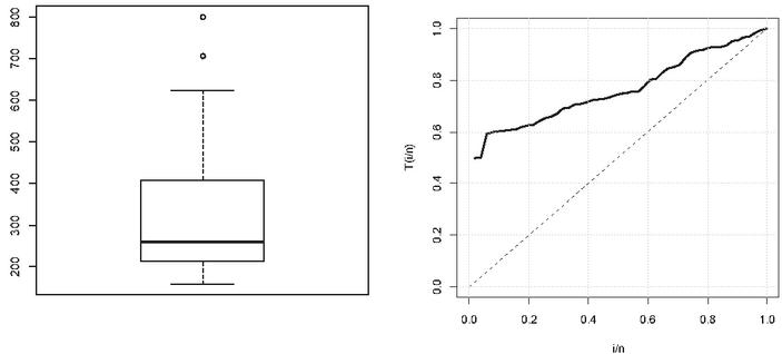
Figure 1 Boxplot and TTT plot of dataset.

Table 8 JCS real data

r	Joint Type II Censored Data
25	158, 159, 189, 191, 192, 193, 194, 195, 198, 200, 202, 207, 212, 215, 220, 229, 230, 235, 237, 240, 244, 245, 247, 250, 256
35	158, 159, 189, 191, 192, 193, 194, 195, 198, 200, 202, 207, 212, 215, 220, 229, 230, 235, 237, 240, 244, 245, 247, 250, 256, 259, 261, 265, 266, 280, 300, 301, 321, 337, 343

Here, $m=22,n=29$. We take $r=25,35$. JCS sample extracted from Table 6 is given in Table 8. MLE and Bayes estimates of parameters are tabulated in Table 9. AL of ACI, Boot-t, Boot-p, BCI, 89% HPD and 95% HPD confidence intervals of all unknown parameters are presented in Table 10. Among classical intervals, ACI gives best interval in terms of shorter length as compared to BOOT-t and BOOT-p for both unknown scale parameters. However, for the unknown shape parameter, BOOT-t gives shortest length interval. Among Bayesian intervals 89%HPD intervals have shortest length than 95%HPD and BCI for all the three unknown parameters. AL of classical (Bayesian) intervals is seen to increase (decrease) with increasing value of r for both the scale parameters while for the unknown shape parameter, AL decreases consistently with increase in r. Figure 2 shows MCMC trace plot of parameters for both values of r.

Table 9 MLE and Bayes estimates of parameters

			Bayes Estimates
r		MLE	SELF	GELF		LINEX		NLINEX
25	${\alpha }_1$	212.3655	210.8308	209.4131	211.2988	139.3936	282.9075	175.1122
	${\alpha }_2$	213.4356	210.5700	209.5355	210.9213	168.7928	283.0064	189.6814
	$\beta$	13.2850	7.6307	7.2492	7.7577	6.0704	9.7957	6.8505
35	${\alpha }_1$	231.8739	231.1812	229.7675	231.6547	187.1820	304.7064	209.1816
	${\alpha }_2$	230.6516	229.0967	227.8632	229.5105	185.8919	281.6296	207.4943
	$\beta$	9.1368	6.4827	6.2682	6.5526	5.6675	7.5724	6.0751

Table 10 AL of different confidence intervals

	r	ACI	BOOT-t	BOOT-p	BCI	HPD89	HPD95
${\alpha }_{\mathbf{1}}$	25	34.390	42.500	35.200	250.393	219.200	236.475
	35	43.451	50.100	47.000	110.900	77.400	99.500
${\alpha }_{\mathbf{2}}$	25	29.091	33.600	29.600	233.927	197.700	228.791
	35	39.962	44.300	41.300	102.500	68.400	97.000
$\beta$	25	8.493	6.940	8.340	10.360	9.052	9.780
	35	5.004	4.329	5.067	4.965	3.835	4.779

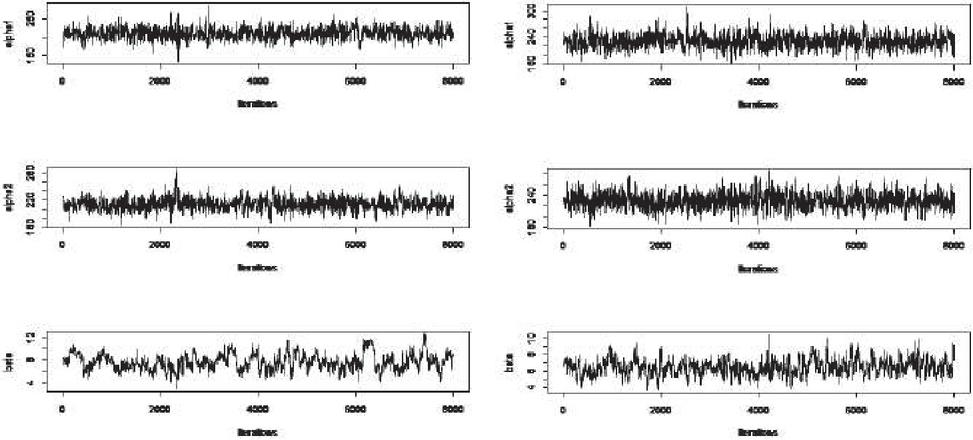
Figure 2 MCMC trace plots of parameters for $r=25,35$.

7 Conclusion

In this paper, classical and Bayesian estimation of parameters under JCS for two contemporary samples is considered when lifetimes follow two distinct log-logistic models with a common shape parameter but different scale parameters. Point and interval Bayes estimates are obtained under a symmetric and four asymmetric loss functions and compared for efficiency relative to the respective classical estimates. As the derived estimators are not in closed form, MCMC iterative technique is used to compute approximate estimates. A real dataset has also been discussed for illustration of the methodology developed in the paper. Simulation study shows that the Bayes estimates perform better than the MLEs in terms of minimum MSE and confidence length. However, MLEs compete closely with the Bayes estimates. Among the interval estimators, HPD intervals are found to be more precise than others in terms of shortest average length.

Acknowledgments

Authors are grateful to the Editor and referees for careful reviewing which greatly strengthened the paper. First author gratefully acknowledges IoE grant from University of Delhi.

References

[1] Abdel-Aty, Y. (2017). Exact likelihood inference for two populations from two-parameter exponential distributions under joint Type-II censoring. Communications in Statistics-Theory and Methods, 46(18), 9026–9041.

[2] Ahsanullah, M., and Alzaatreh, A. (2018). Parameter estimation for the log-logistic distribution based on order statistics. REVSTAT, 16(4), 429–443.

[3] Aldrich, J. (1997). RA Fisher and the making of maximum likelihood 1912–1922. Statistical Science, 12(3), 162–176.

[4] Al-Matrafi, B. N., and Abd-Elmougod, G. A. (2017). Statistical inferences with jointly type-II censored samples from two rayleigh distributions. Global Journal of Pure and Applied Mathematics, 13(12), 8361–8372.

[5] Al-Shomrani, A. A., Shawky, A. I., Arif, O. H., and Aslam, M. (2016). Log-logistic distribution for survival data analysis using MCMC. SpringerPlus, 5(1), 1–16.

[6] Ashkar, F., and Mahdi, S. (2006). Fitting the log-logistic distribution by generalized moments. Journal of Hydrology, 328(3–4), 694–703.

[7] Ashour, S. K., and Abo-Kasem, O. E. (2014). Parameter estimation for two Weibull populations under joint Type II censored scheme. International Journal of Engineering, 5(04), 8269.

[8] Ashour, S. K., and Abo-Kasem, O. E. (2014). Bayesian and non–Bayesian estimation for two generalized exponential populations under joint type II censored scheme. Pakistan Journal of Statistics and Operation Research, 57–72.

[9] Balakrishnan, N., and Rasouli, A. (2008). Exact likelihood inference for two exponential populations under joint Type-II censoring. Computational Statistics & Data Analysis, 52(5), 2725–2738.

[10] Balakrishnan, N., and Su, F. (2015). Exact likelihood inference for k exponential populations under joint type-II censoring. Communications in Statistics-Simulation and Computation, 44(3), 591–613.

[11] Berger, J. O. (1985). Prior information and subjective probability. In Statistical Decision Theory and Bayesian Analysis (pp. 74–117). Springer, New York, NY.

[12] Calabria, R., and Pulcini, G. (1996). Point estimation under asymmetric loss functions for left-truncated exponential samples. Communications in Statistics-Theory and Methods, 25(3), 585–600.

[13] Chehade, A., Shi, Z., and Krivtsov, V. (2020). Power–law nonhomogeneous Poisson process with a mixture of latent common shape parameters. Reliability Engineering & System Safety, 203, 107097.

[14] Collett, D. (2015). Modelling survival data in medical research. CRC press.

[15] Fisk, P. R. (1961). The graduation of income distributions. Econometrica: journal of the Econometric Society, 171–185.

[16] Guure, C. B. (2015). Inference on the loglogistic model with right censored data. Austin Biom and Biostat, 2(1), 1015.

[17] Hastings, W. K. (1970). Monte Carlo sampling methods using Markov chains and their applications. Biometrika, 57(1), 97–109.

[18] Hoel, D. G. (1972). A representation of mortality data by competing risks. Biometrics, 475–488.

[19] Islam, A. F. M., Roy, M. K., and Ali, M. M. (2004). A Non-Linear Exponential (NLINEX) Loss Function in Bayesian Analysis. Journal of the Korean Data and Information Science Society, 15(4), 899–910.

[20] Jeffreys, H. (1961). Theory of probability: Oxford university press. New York, 472.

[21] Lawless, J. F. (2003). Copyright© 2003 John Wiley & Sons, Inc. Statistical Models and Methods for Lifetime Data, 3, 577.

[22] Metropolis, N., A.W. Rosenbluth, M.N. Rosenbluth, A.H. Teller and E. Teller. (1953). Equation of state calculations by fast computing machines. Journal of Chemical Physics, 21(6): 1087–1091. DOI: 10.1063/1.1699114

[23] Nelson, W. B. (2003). Recurrent Events Data Analysis for Product Repairs, Disease Recurrences, and Other Applications. Society for Industrial and Applied Mathematics.

[24] Nelson, W. B. (2009). Accelerated Testing: Statistical Models, Test Plans, and Data Analysis (Vol. 344). John Wiley & Sons.

[25] Panza, C. A., and Vargas, J. A. (2016). Monitoring the shape parameter of a Weibull regression model in phase II processes. Quality and Reliability Engineering International, 32(1), 195–207.

[26] Reath, J., Dong, J., and Wang, M. (2018). Improved parameter estimation of the log-logistic distribution with applications. Computational Statistics, 33(1), 339–356.

[27] Sewailem, M. F., and Baklizi, A. (2019). Inference for the log-logistic distribution based on an adaptive progressive type-II censoring scheme. Cogent Mathematics & Statistics, 6(1), 1684228.

[28] Singh, V. P., and Guo, H. (1995). Parameter estimation for 2-parameter log-logistic distribution (LLD2) by maximum entropy. Civil Engineering Systems, 12(4), 343–357.

[29] Shafay, A. R., Balakrishnan, N., and Abdel-Aty, Y. (2014). Bayesian inference based on a jointly type-II censored sample from two exponential populations. Journal of Statistical Computation and Simulation, 84(11), 2427–2440.

[30] Shoukri, M. M., Mian, I. U. H., and Tracy, D. S. (1988). Sampling properties of estimators of the log-logistic distribution with application to Canadian precipitation data. Canadian Journal of Statistics, 16(3), 223–236.

[31] Tripathy, M. R., and Nagamani, N. (2017). Estimating common shape parameter of two gamma populations: A simulation study. Journal of Statistics and Management Systems, 20(3), 369–398.

[32] Varian, H. R. (1975). A Bayesian approach to real estate assessment. Studies in Bayesian Econometric and Statistics in Honor of Leonard J. Savage, 195–208.

[33] Voorn, W. J. (1987). Characterization of the logistic and loglogistic distributions by extreme value related stability with random sample size. Journal of Applied Probability, 24(4), 838–851.

Biographies

Ranjita Pandey is an esteemed faculty at Department of Statistics, University of Delhi, Delhi. She has more than 20 years of experience of teaching and research. Her research areas include theoretical and applied Bayesian Inference, lifetime distributions, time series models, demography, imputation methods and ecological modelling. She has extensive administrative experience. She has delivered many invited lectures and has served as reviewer for several journals.

Pulkit Srivastava is currently pursuing his Ph.D. at the Department of Statistics, University of Delhi, Delhi. His research areas include Bayesian Inference, Stochastic processes etc.

Journal of Reliability and Statistical Studies, Vol. 15, Issue 1 (2022), 229–260.
doi: 10.13052/jrss0974-8024.15110
© 2022 River Publishers