The Unit Folded Normal Distribution: A New Unit Probability Distribution with the Estimation Procedures, Quantile Regression Modeling and Educational Attainment Applications

Mustafa Ç. Korkmaz¹, Christophe Chesneau^2,* and Zehra Sedef Korkmaz³

¹Department of Measurement and Evaluation, Artvin Çoruh University, City Campus, Artvin, 08000, Turkey
²LMNO, University of Caen Normandie, Caen, 14032, France
³Department of Curriculum and Instruction Program, Artvin Çoruh University, City Campus, Artvin, 08000, Turkey
E-mail: mustafacagataykorkmaz@gmail.com; christophe.chesneau@gmail.com; zehrasedefcoskun@gmail.com
*Corresponding Author

Received 09 September 2021; Accepted 04 April 2022; Publication 25 April 2022

Abstract

In this paper, we develop a continuous distribution on the unit interval characterized by the distribution of the absolute hyperbolic tangent transformation of a random variable following the normal distribution. The lack of research on the prospect of hyperbolic transformations providing flexible distributions on the unit interval is a motivation for the study. First, we study it theoretically and discuss its properties of interest from a modeling point of view. In particular, it is shown that the proposed distribution accommodates various levels of skewness and kurtosis. Then, some statistical work is performed. We investigate diverse estimation methods for the involved parameters and evaluate their performance through two simulation studies. Subsequently, the quantile regression model derived from the proposed distribution is developed. Two real-world data applications of interest are provided. The first application is about the univariate modeling of the percentage of the educational attainment of some countries, which is one indicator of the education topic of the Better Life Index (BLI) of the Organization for Economic Co-operation and Development (OECD) countries. The second application is to explain the relationship between the percentage of educational attainment of some countries with one indicator of the work-life balance, safety, and health topics of BLI via median quantile regression modeling. For the considered data sets, the proposed distribution and quantile regression models show that they have better modeling abilities than competitive models under some comparison criteria. The results also indicate that covariates are (statistically) significant at any ordinary level of significance for the median response.

Keywords: Better life index, educational attainment, hyperbolic tangent function, normal distribution, point estimates, OECD data sets, quantile regression, unit distribution.

1 Introduction

BLI has been proposed by the OECD to define the measure of well-being of different countries. It includes many metrics, such as social, economic, and environmental performance. By empowering citizens in the policy-making process, BLI aims to educate citizens on measuring the well-being of societies by empowering citizens in the policy-making process.

The BLIs of the countries consist of 11 topics such as income, jobs, housing, community, safety, education, environment, civil engagement, life satisfaction, health, and work-life balance. Each of the 11 variables of the index is currently based on one to three indicators. For example, the education variable consists of the educational attainment, student skills, and years of education indicators of the related countries. Further, the subject of these indicators has been used to relate to other indicators in the literature. In particular, the educational attainment indicator has been the subject of many studies.

According to the BLI variable of the OECD, educational attainment is specified as the highest score obtained at the most advanced level attended in the education system of the country where the education was received. The level of education takes into account the number of adults aged 25 to 64 with at least an upper secondary school diploma in the population of the same age. The unit of this measurement is given as the percentage of the adult population (aged 25 to 64) in the BLI. Adams [3] has found an education-health relationship in older people, even after taking into account individual and family characteristics, and he has examined to what extent this relationship represents an independent effect of education on health. Abel and Kruger [2] have examined the relationship between educational attainment and the suicide rate in the United States for the year 2001. Hill and Needham [22] have tested whether the self-rated health indicator improved over time (from 1972 to 2002) for women and men, and they also examined the extent to which historical gains in health were maintained. The educational attainment indicator helps explain any trends observed using ordered logistic regression. Gyekye and Salminen [20] have examined the relationship between educational attainment and perceptions of safety, job satisfaction, adherence to safety management policies, and the frequency of accidents via various statistical test procedures. Borgonovi and Pokropek [8] have examined the contribution of human capital to health in 23 countries around the world using the OECD Survey of Adult Skills, a unique large-scale international assessment of 1-65 year olds that contains information on self-reported health status, cognitive skills, education, and indicators of interpersonal confidence. This represents the cognitive dimension of social capital. Hazekamp et al. [21] have conducted a temporal trend analysis examining the educational attainment of male homicide victims aged 18 to 24 in the city of Chicago from 2006 to 2015 to describe the educational attainment of young victims of homicide in Chicago. Schellekens and Ziv [41] have tried to explain long-term trends in self-rated (reported) health with gender, age, race, and education covariates using regression analysis in the United States. Using the BLI topics, Altun [4] has given two applications via the regression approach. The first concerns the relationship between educational attainment values in OECD countries and indicators of the homicide rate and labor market insecurity. The other concerns the relationship between self-reported health status and indicators of water quality, air pollution, and homicide rate via regression modeling of the unit mean response. In general, these articles were motivated by the link between education level and other variables (indicators).

On the other hand, modeling real-world phenomena with probability models is very important for the statistical inference based on these phenomena. This issue has been studied by many statisticians and it continues to be studied. In particular, unit interval modeling approaches have increased recently as they are related to certain issues such as recovery and mortality rates, and the proportion of educational attainment, etc. based on the different world countries. When researchers want inferences about these important questions, the beta distribution comes to mind directly. Although the beta distribution has a probability density function (PDF) that is flexible in nature, it is sometimes not sufficient to model and explain all the informative characteristics of unit data sets. For this reason, in order to assess whether there are better results than the beta distribution based on statistical inference, new alternative models have been defined on the unit interval. Current literature on this topic includes $\text{Johnson}{S}_B$ [25], Topp-Leone [44], Kumaraswamy [30], generalized beta [36], standard two-sided power distribution [45], log-Lindley [18], log-xgamma [7], unit Birnbaum-Saunders [33], unit Lindley [31], unit inverse Gaussian [17], unit Gompertz [32], log-weighted exponential [4], $2^{nd}$ degree unit Lindley [5], logit slash [26], unit generalized half normal [27], unit Johnson $S_U$ [19], unit Burr-XII [28] and trapezoidal beta [14] distributions. Many of the above distributions were obtained via transforming a parent distribution, and most of them gave better results than the beta distribution from a modeling point of view. In addition, for some of the distributions introduced above, alternative regression models have been derived. It is well-known that the beta regression has been proposed by [12], the Kumaraswamy quantile regression model has been introduced by [37], the unit-Lindley regression model has been studied by [31]. Also, Reference [4] proposed a regression model alternative to the beta regression model based on the weighted-exponential distribution. A flexible alternative regression model has been elaborated by [5] for the beta and simplex regression models. The unit-Weibull quantile regression (QR) model has been introduced by [35] as an alternative model to the beta and Kumaraswamy QR models. Last but not least, the log-extended exponential-geometric QR model developed by [24] also appears to be a serious competitor.

The objective of this study is to propose an original unit competitive distribution and its QR modeling to deal with percentages and proportions with their applications based on the proportion of the educational attainments’ OECD countries. We are also motivated to relate educational attainments’ OECD countries with covariates, which are some indicators of BLI topics such as work-life balance, safety, and health. To obtain a new ‘unit distribution’, we use a novel transformation of the normal distribution. This transformation is based on the absolute version of the hyperbolic tangent function. To our knowledge, this direction of research remains almost unexplored in the literature on unit distributions, despite the interest of hyperbolic functions in various branches of probability and statistical modeling (see [13]). “Almost” because, to our knowledge, in this framework, only the arcsecant normal distribution by [29] uses such an approach. Here, we motivate the fact that the considered transformation is able to carry the applicability of the normal distribution to the unit interval. It can be also noted that although a lot of distributions are proposed in order to analyze data on the $(0,1)$ unit interval, using the same models for every problem is not useful. In this sense, proposing new distributions is welcome and is applied.

The frame of the paper is as follows: The new distribution is described in Section 2. Some of its characteristics are specified by Section 3. Section 4 is dedicated to the estimation of the related model parameters, including simulation work. The new QR model based on the newly defined distribution, as well as its residual analysis, are explored in Section 5. Section 6 discusses univariate data modeling and QR modeling applications. Finally, the article ends with some comments in Section 7.

2 The ‘$UFN$ distribution’

We start with a normal random variable (RV): $Y\sim N(\mu ,{\sigma }^2)$, where $\mu \in ℝ$ denotes the mean of $Y$ and $\sigma >0$ its standard deviation. We define $X=\left|\tanh Y\right|$, where $\tanh y=(e^y-e^{-y})/(e^y+e^{-y})$, $y\in ℝ$. We denote the distribution of $X$ by the expression $UFN$ for ‘unif folded normal’ or $UFN(\mu ,\sigma )$ where the mention of the two related parameters $\mu$ and $\sigma$ has an interest. Consequently, because of the transformation considered, the $UFN$ distribution is a unit distribution. To our knowledge, it is new in the literature, and the underlying motivations are developed in several parts of the remainder of the study. As the first elements, the next result presents the related cumulative distribution function (CDF) and PDF, respectively.

Proposition 1.

First, for $x\mathrm{\in }\mathrm{(}\mathrm{0}\mathrm{,}\mathrm{1}\mathrm{)}$, the CDF of the $U\mathit{}F\mathit{}N$ distribution is determined as

$F(x,\mu ,\sigma )=\mathrm{\Phi }\left({\displaystyle \frac{\mathrm{arctanh}x+\mu }{\sigma }}\right)+\mathrm{\Phi }\left({\displaystyle \frac{\mathrm{arctanh}x-\mu }{\sigma }}\right)-1,$

(1)

where $\mathrm{\Phi }\mathit{}\mathrm{(}x\mathrm{)}$ is the CDF of the standard normal ($N\mathit{}\mathrm{(}\mathrm{0}\mathrm{,}\mathrm{1}\mathrm{)}$) distribution and $\mathrm{arctanh}\mathit{}x$ is the inverse function of $\tanh \mathit{}x$. Also, for $x\mathrm{\in }\mathrm{(}\mathrm{0}\mathrm{,}\mathrm{1}\mathrm{)}$, the related PDF is

$f(x,\mu ,\sigma )={\displaystyle \frac{1}{\sigma \left(1-x^2\right)}}\left[\varphi \left({\displaystyle \frac{\mathrm{arctanh}x+\mu }{\sigma }}\right)+\varphi \left({\displaystyle \frac{\mathrm{arctanh}x-\mu }{\sigma }}\right)\right],$

where $\varphi \mathit{}\mathrm{(}x\mathrm{)}$ is the PDF of the $N\mathit{}\mathrm{(}\mathrm{0}\mathrm{,}\mathrm{1}\mathrm{)}$ distribution. For $x\mathrm{\notin }\mathrm{(}\mathrm{0}\mathrm{,}\mathrm{1}\mathrm{)}$, we complete the functions $F\mathit{}\mathrm{(}x\mathrm{,}\mu \mathrm{,}\sigma \mathrm{)}$ and $f\mathit{}\mathrm{(}x\mathrm{,}\mu \mathrm{,}\sigma \mathrm{)}$ as usual.

Proof.

Owing to the representation $X=\left|\tanh Y\right|$ with $Y\sim N(\mu ,{\sigma }^2)$, the CDF of $X$ can be developed as

$P(X\le x)$	$=P(-x\le \tanh Y\le x)$
	$=P(\mathrm{arctanh}(-x)\le Y\le \mathrm{arctanh}x)$
	$=P(-\mathrm{arctanh}x\le Y\le \mathrm{arctanh}x)$
	$=\mathrm{\Phi }\left({\displaystyle \frac{\mathrm{arctanh}x-\mu }{\sigma }}\right)-\mathrm{\Phi }\left({\displaystyle \frac{-\mathrm{arctanh}x-\mu }{\sigma }}\right)$
	$=\mathrm{\Phi }\left({\displaystyle \frac{\mathrm{arctanh}x-\mu }{\sigma }}\right)$
	$\mathrm{\hspace{1em}}-\left[1-\mathrm{\Phi }\left(-{\displaystyle \frac{-\mathrm{arctanh}x-\mu }{\sigma }}\right)\right]$
	$=\mathrm{\Phi }\left({\displaystyle \frac{\mathrm{arctanh}x+\mu }{\sigma }}\right)+\mathrm{\Phi }\left({\displaystyle \frac{\mathrm{arctanh}x-\mu }{\sigma }}\right)-1.$

The desired expression for $F(x,\mu ,\sigma )$ is obtained. The expression of $f(x,\mu ,\sigma )$ follows by differentiating $F(x,\mu ,\sigma )$ according to $x$, ending the proof. ∎

Based on Proposition 1, for $x\in (0,1)$, the following relations hold:

$F(x,0,\sigma )=2\mathrm{\Phi }\left({\displaystyle \frac{1}{\sigma }}\mathrm{arctanh}x\right)-1,$

$f(x,0,\sigma )={\displaystyle \frac{2}{\sigma \left(1-x^2\right)}}\varphi \left({\displaystyle \frac{1}{\sigma }}\mathrm{arctanh}x\right).$

Also, another expression for the PDF is

$$f(x,\mu ,\sigma )=\sqrt{\frac{2}{\pi }}\frac{1}{\sigma \left(1-x^2\right)}{e}^{-\frac{{\left(\mathrm{arctanh}x\right)}^2+{\mu }^2}{2{\sigma }^2}}\cosh \left(\frac{\mu }{{\sigma }^2}\mathrm{arctanh}x\right),$$

(3)

where $\cosh y=(e^y+e^{-y})/2$. When $x$ tends to $0$, we get $f(x,\mu ,\sigma )=\sqrt{2/\pi }(1/\sigma )e^{-\frac{{\mu }^2}{2{\sigma }^2}}$, which is a decreasing function with respect to $|\mu |$. Also, from Equation (1), for $x\in (0,1)$, we notice that

$f(x,-\mu ,\sigma )$	$={\displaystyle \frac{1}{\sigma \left(1-x^2\right)}}\left[\varphi \left({\displaystyle \frac{\mathrm{arctanh}x-\mu }{\sigma }}\right)+\varphi \left({\displaystyle \frac{\mathrm{arctanh}x+\mu }{\sigma }}\right)\right]$
	$=f(x,\mu ,\sigma ).$

This implies that the $UFN(\mu ,\sigma )$ and $UFN(-\mu ,\sigma )$ distributions coincide. On another plan, the $UFN$ distribution can be unimodal, with a mode into $(0,1)$. It can be determined by solving the following nonlinear equation according to $x$:

$$2{\sigma }^{2}x-\mathrm{arctanh}(x)+\mu \tanh \left(\frac{\mu }{{\sigma }^2}\mathrm{arctanh}x\right)=0.$$

The complexity of this equation is certain; a numerical treatment is required to determine the solution.

Among the important survival functions, the hazard rate function (HRF) of the $UFN(\mu ,\sigma )$ distribution is expressed as

$h(x,\mu ,\sigma )={\displaystyle \frac{\varphi \left(\frac{\mathrm{arctanh}x+\mu }{\sigma }\right)+\varphi \left(\frac{\mathrm{arctanh}x-\mu }{\sigma }\right)}{\sigma \left(1-x^2\right)\left[2-\mathrm{\Phi }\left(\frac{\mathrm{arctanh}x+\mu }{\sigma }\right)-\mathrm{\Phi }\left(\frac{\mathrm{arctanh}x-\mu }{\sigma }\right)\right]}}$

for $x\in (0,1)$. For $x\notin (0,1)$, standard completions on $h(x,\mu ,\sigma )$ are applied. When $x$ tends to $0$, we have $h(x,\mu ,\sigma )\sim f(x,\mu ,\sigma )=\sqrt{2/\pi }(1/\sigma )e^{-\frac{{\mu }^2}{2{\sigma }^2}}$, which is a decreasing function with respect to $|\mu |$. Figure 1 displays some curves of $f(x,\mu ,\sigma )$ and $h(x,\mu ,\sigma )$ for some chosen values of the parameters.

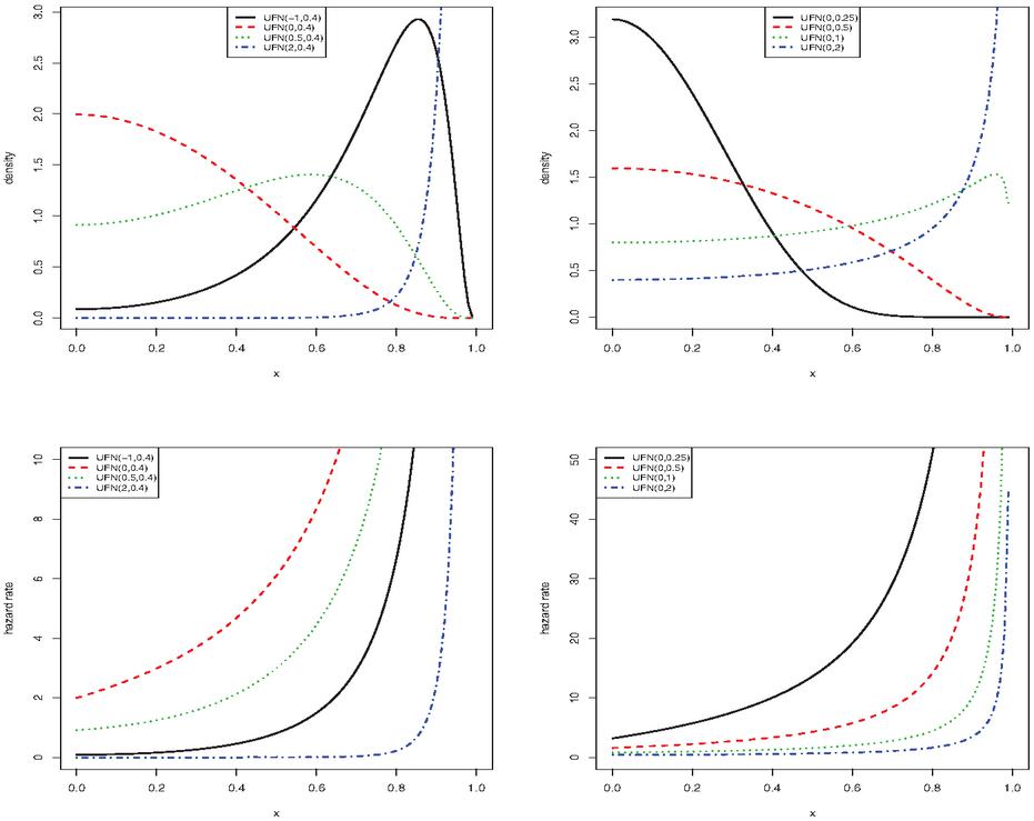
Figure 1 Samples of PDF and HRF shapes of the $UFN$ distribution.

Figure 1 shows that the $UFN$ distribution is very flexible; its PDF possesses a large panel of forms, including increasing, decreasing, bell-reversed bathtubs, and almost constant shapes. Also, we observe that the HRF is exclusively J shaped. This flexibility demonstrates that the $UFN$ distribution is able to model various phenomena with values in $(0,1)$, and should be considered a serious option in this regard. Some of these modeling aspects are examined in the next parts of the study.

3 Notable Properties

The $UFN$ distribution is deeply related to the normal distribution, which makes it easier to study some of these important properties. Some of them are covered in this section.

3.1 Stochastic ordering

As a first approach, the $UFN$ distribution satisfies some stochastic ordering properties as described in full generality in [42]. As an immediate fact, the following stochastic dominance holds. For any ${\sigma }_2>{\sigma }_1$, based on Equation (1), since the CDF $\mathrm{\Phi }(x)$ is increasing, we have $F(x,{\sigma }_2,0)\le F(x,{\sigma }_1,0)$. We now discuss a monotone likelihood ratio property of the $UFN$ distribution. Let $X_1\sim UFN(\mu ,{\sigma }_1)$, $X_2\sim UFN(\mu ,{\sigma }_2)$, and $g(x)$ be the ratio function defined by the respective PDFs, that is, by using Equation (3),

$g(x)={\displaystyle \frac{f(x,\mu ,{\sigma }_1)}{f(x,\mu ,{\sigma }_2)}}$

$={\displaystyle \frac{{\sigma }_2}{{\sigma }_1}}{e}^{-\frac{{\left(\mathrm{arctanh}x\right)}^2+{\mu }^2}{2}\left(\frac{1}{{\sigma }_1^2}-\frac{1}{{\sigma }_2^2}\right)}{\displaystyle \frac{\cosh \left(\frac{\mu }{{\sigma }_1^2}\mathrm{arctanh}x\right)}{\cosh \left(\frac{\mu }{{\sigma }_2^2}\mathrm{arctanh}x\right)}}.$

Then, we have

$\log \left[g(x)\right]$	$=\log \left({\displaystyle \frac{{\sigma }_2}{{\sigma }_1}}\right)-{\displaystyle \frac{{\left(\mathrm{arctanh}x\right)}^2+{\mu }^2}{2}}\left({\displaystyle \frac{1}{{\sigma }_1^2}}-{\displaystyle \frac{1}{{\sigma }_2^2}}\right)$
	$\mathrm{\hspace{1em}}+\log \left[{\displaystyle \frac{\cosh \left(\frac{\mu }{{\sigma }_1^2}\mathrm{arctanh}x\right)}{\cosh \left(\frac{\mu }{{\sigma }_2^2}\mathrm{arctanh}x\right)}}\right]$

and

${\displaystyle \frac{d}{dx}}\log \left[g(x)\right]$	$=-{\displaystyle \frac{\mathrm{arctanh}x}{1-x^2}}\left({\displaystyle \frac{1}{{\sigma }_1^2}}-{\displaystyle \frac{1}{{\sigma }_2^2}}\right)+\mu {\displaystyle \frac{1}{1-x^2}}$
	$\mathrm{\hspace{1em}}\times \left[{\displaystyle \frac{1}{{\sigma }_1^2}}\tanh \left({\displaystyle \frac{\mu }{{\sigma }_1^2}}\mathrm{arctanh}x\right)-{\displaystyle \frac{1}{{\sigma }_2^2}}\tanh \left({\displaystyle \frac{\mu }{{\sigma }_2^2}}\mathrm{arctanh}x\right)\right].$

If we focus on the two main terms of this difference, one can notice that the function $r(y)=(1/y)\tanh [(\mu /y)\mathrm{arctanh}x]$ is decreasing with respect to $y$, contrary to $-1/y$, implying that there is no immediate result on the sign of $d\log \left[g(x)\right]/dx$ according to ${\sigma }_2>{\sigma }_1$ or ${\sigma }_2<{\sigma }_1$. However, when $\mu$ tends to $0$, the following equivalence holds:

${\displaystyle \frac{d}{dx}}\log \left[g(x)\right]$

$\sim -{\displaystyle \frac{\mathrm{arctanh}x}{1-x^2}}\left({\displaystyle \frac{1}{{\sigma }_1^2}}-{\displaystyle \frac{1}{{\sigma }_2^2}}\right)\left[1-{\mu }^2\left({\displaystyle \frac{1}{{\sigma }_1^2}}+{\displaystyle \frac{1}{{\sigma }_2^2}}\right)\right],$

and this last function is nonnegative for ${\sigma }_1>{\sigma }_2$. This establishes the existence of a constant $c$ such that, if $|\mu |\le c$ and ${\sigma }_1>{\sigma }_2$, $g(x)$ is nondecreasing, implying that the $UFN$ distribution satisfies the monotone likelihood ratio property in this setting; the higher the observed value, the more likely it is to come from $X_1$ rather than $X_2$.

3.2 Generation of the Random Numbers

Generating $n$ values from the $UFN$ distribution is straightforward thanks to its mathematical structure. Indeed, since $X=\left|\tanh Y\right|\sim UFN(\mu ,\sigma )$, where $Y\sim N(\mu ,{\sigma }^2)$, it is enough to generate $n$ values from the classic $N(\mu ,{\sigma }^2)$ distribution, say $x_1,x_2,\mathrm{\dots },x_n$, then $n$ values from the $UFN$ distribution are given by $y_1,y_2,\mathrm{\dots },y_n$, where $y_i=|\tanh (x_i)|$ for $i=1,\mathrm{\dots },n$.

3.3 Quantile Function

The quantile function (QF) of a distribution completely identifies the distribution. It is the main ingredient of various probabilistic objects and statistical tools. The QF of the $UFN$ distribution is defined by the inverse of $F(x,\mu ,\sigma )$ as presented in Equation (1). That is, it is the function $Q(u,\mu ,\sigma )$ such that $F[Q(u,\mu ,\sigma )]=u$ for $u\in (0,1)$, or equivalently,

$$\mathrm{\Phi }\left(\frac{\mathrm{arctanh}[Q(u,\mu ,\sigma )]+\mu }{\sigma }\right)+\mathrm{\Phi }\left(\frac{\mathrm{arctanh}[Q(u,\mu ,\sigma )]-\mu }{\sigma }\right)=1+u.$$

In the special case $\mu =0$, the QF has the following closed form:

$$Q(u,0,\sigma )=\tanh \left[\sigma {\mathrm{\Phi }}^{-1}\left(\frac{1+u}{2}\right)\right],$$

where ${\mathrm{\Phi }}^{-1}(x)$ is the inverse function of $\mathrm{\Phi }(x)$ (corresponding to the QF of the $N(0,1)$ distribution). From this expression, the quartiles of the $UFN$ distribution follow:

$$Q_1=\tanh \left[\sigma {\mathrm{\Phi }}^{-1}\left(\frac{5}{8}\right)\right],Q_2=\tanh \left[\sigma {\mathrm{\Phi }}^{-1}\left(\frac{3}{4}\right)\right],$$

$$Q_3=\tanh \left[\sigma {\mathrm{\Phi }}^{-1}\left(\frac{7}{8}\right)\right],$$

with ${\mathrm{\Phi }}^{-1}\left(5/8\right)\approx 0.3186394$, ${\mathrm{\Phi }}^{-1}\left(3/4\right)\approx 0.6744898$ and ${\mathrm{\Phi }}^{-1}\left(7/8\right)\approx 1.150349$. In addition, thanks to the QF, one can introduce various measures of asymmetry and kurtosis, such as those proposed in [16] and [38].

3.4 Moments

Since the $UFN$ distribution is unit-support, the moments of any order exist automatically. Since no closed form expression exists for them, a manageable series expansion is provided in the next proposition.

Proposition 2.

Firstly, let $U$ be a RV following the $N\mathit{}\mathrm{(}\mathrm{0}\mathrm{,}\mathrm{1}\mathrm{)}$ distribution. We define the truncated moment generating function of $U$ as $M_a\mathrm{(}t\mathrm{)}\mathrm{=}E\mathrm{\left[}{e}^{t\mathit{}U}I\mathrm{(}U\mathrm{>}a\mathrm{)}\mathrm{\right]}$, $t\mathrm{,}a\mathrm{\in }\mathrm{R}$, and $I\mathrm{(}U\mathrm{>}a\mathrm{)}\mathrm{=}\mathrm{1}$ if $\mathrm{\{}U\mathrm{>}a\mathrm{\}}$ is realized, and $\mathrm{0}$ otherwise. Now, let $m$ be a positive integer and $X\mathrm{\sim }U\mathit{}F\mathit{}N\mathit{}\mathrm{(}\mu \mathrm{,}\sigma \mathrm{)}$. Then, the $m$-th moment of $X$ can be expressed as

${\theta }_m$	$=E(X^m)={\displaystyle \sum _{k=0}^m}{\displaystyle \sum _{\mathrm{\ell }=0}^{+\mathrm{\infty }}}\left({\displaystyle \genfrac{}{}{0pt}{}{m}{k}}\right)\left({\displaystyle \genfrac{}{}{0pt}{}{-k}{\mathrm{\ell }}}\right){(-1)}^k{2}^k$
	$\mathrm{\hspace{1em}}\times \left[e^{-2(k+\mathrm{\ell })\mu }{M}_{-\frac{\mu }{\sigma }}(-2(k+\mathrm{\ell })\sigma )+e^{2\mathrm{\ell }\mu }{M}_{\frac{\mu }{\sigma }}(-2\mathrm{\ell }\sigma )\right].$

Proof.

From the representation $X=\left|\tanh Y\right|$, where $Y\sim N(\mu ,{\sigma }^2)$, we can write ${\theta }_m=E({|\tanh Y|}^m)$. Now, let us show that

${[\tanh y]}^m$	$={\displaystyle \sum _{k=0}^m}{\displaystyle \sum _{\mathrm{\ell }=0}^{+\mathrm{\infty }}}\left({\displaystyle \genfrac{}{}{0pt}{}{m}{k}}\right)\left({\displaystyle \genfrac{}{}{0pt}{}{-k}{\mathrm{\ell }}}\right){(-1)}^k{2}^k$
	$\mathrm{\hspace{1em}}\times [e^{-2(k+\mathrm{\ell })y}I(y>0)+e^{2\mathrm{\ell }y}I(y<0)].$	(5)

The formula is straightforward for $y=0$. For $y>0$, the binomial formula yields

${[\tanh y]}^m$	$={\left({\displaystyle \frac{e^y-e^{-y}}{e^y+e^{-y}}}\right)}^m={\left(1-2{\displaystyle \frac{e^{-2y}}{1+e^{-2y}}}\right)}^m$
	$={\displaystyle \sum _{k=0}^m}\left({\displaystyle \genfrac{}{}{0pt}{}{m}{k}}\right){(-1)}^k{2}^k{e}^{-2ky}{(1+e^{-2y})}^{-k}$
	$={\displaystyle \sum _{k=0}^m}{\displaystyle \sum _{\mathrm{\ell }=0}^{+\mathrm{\infty }}}\left({\displaystyle \genfrac{}{}{0pt}{}{m}{k}}\right)\left({\displaystyle \genfrac{}{}{0pt}{}{-k}{\mathrm{\ell }}}\right){(-1)}^k{2}^k{e}^{-2(k+\mathrm{\ell })y}.$

Also, for $y<0$, by the same argument, we get

${[\tanh y]}^m$	$={\left({\displaystyle \frac{e^y-e^{-y}}{e^y+e^{-y}}}\right)}^m={\left(1-2{\displaystyle \frac{1}{1+e^{2y}}}\right)}^m$
	$={\displaystyle \sum _{k=0}^m}\left({\displaystyle \genfrac{}{}{0pt}{}{m}{k}}\right){(-1)}^k{2}^k{(1+e^{2y})}^{-k}$
	$={\displaystyle \sum _{k=0}^m}{\displaystyle \sum _{\mathrm{\ell }=0}^{+\mathrm{\infty }}}\left({\displaystyle \genfrac{}{}{0pt}{}{m}{k}}\right)\left({\displaystyle \genfrac{}{}{0pt}{}{-k}{\mathrm{\ell }}}\right){(-1)}^k{2}^k{e}^{2\mathrm{\ell }y}.$

The desired formula follows by putting the two equalities together. Therefore, by Equation (3.4) and the dominated convergence theorem, we can write

${\theta }_m$	$={\displaystyle \sum _{k=0}^m}{\displaystyle \sum _{\mathrm{\ell }=0}^{+\mathrm{\infty }}}\left({\displaystyle \genfrac{}{}{0pt}{}{m}{k}}\right)\left({\displaystyle \genfrac{}{}{0pt}{}{-k}{\mathrm{\ell }}}\right){(-1)}^k{2}^k$
	$\mathrm{\hspace{1em}}\times [E(e^{-2(k+\mathrm{\ell })Y}I(Y>0))+E(e^{2\mathrm{\ell }Y}I(Y<0))].$

Now, since $Y\sim N(\mu ,{\sigma }^2)$, we have $Y=\mu +\sigma U$ where $U\sim N(0,1)$, in the distribution sense. Therefore, we have

${\theta }_m$	$={\displaystyle \sum _{k=0}^m}{\displaystyle \sum _{\mathrm{\ell }=0}^{+\mathrm{\infty }}}\left({\displaystyle \genfrac{}{}{0pt}{}{m}{k}}\right)\left({\displaystyle \genfrac{}{}{0pt}{}{-k}{\mathrm{\ell }}}\right){(-1)}^k{2}^k$
	$\mathrm{\hspace{1em}}\times [e^{-2(k+\mathrm{\ell })\mu }E\left\{e^{-2(k+\mathrm{\ell })\sigma U}I(U>-{\displaystyle \frac{\mu }{\sigma }})\right\}$
	$\mathrm{\hspace{1em}}+e^{2\mathrm{\ell }\mu }E\left\{e^{2\mathrm{\ell }\sigma U}I(U<-{\displaystyle \frac{\mu }{\sigma }})\right\}]$
	$={\displaystyle \sum _{k=0}^m}{\displaystyle \sum _{\mathrm{\ell }=0}^{+\mathrm{\infty }}}\left({\displaystyle \genfrac{}{}{0pt}{}{m}{k}}\right)\left({\displaystyle \genfrac{}{}{0pt}{}{-k}{\mathrm{\ell }}}\right){(-1)}^k{2}^k$
	$\mathrm{\hspace{1em}}\times [e^{-2(k+\mathrm{\ell })\mu }E\left\{e^{-2(k+\mathrm{\ell })\sigma U}I(U>-{\displaystyle \frac{\mu }{\sigma }})\right\}$
	$\mathrm{\hspace{1em}}+e^{2\mathrm{\ell }\mu }E\left\{e^{-2\mathrm{\ell }\sigma U}I(U>{\displaystyle \frac{\mu }{\sigma }})\right\}]$
	$={\displaystyle \sum _{k=0}^m}{\displaystyle \sum _{\mathrm{\ell }=0}^{+\mathrm{\infty }}}\left({\displaystyle \genfrac{}{}{0pt}{}{m}{k}}\right)\left({\displaystyle \genfrac{}{}{0pt}{}{-k}{\mathrm{\ell }}}\right){(-1)}^k{2}^k$
	$\mathrm{\hspace{1em}}\times \left[e^{-2(k+\mathrm{\ell })\mu }{M}_{-\frac{\mu }{\sigma }}(-2(k+\mathrm{\ell })\sigma )+e^{2\mathrm{\ell }\mu }{M}_{\frac{\mu }{\sigma }}(-2\mathrm{\ell }\sigma )\right].$

The desired result is obtained. ∎

The mean and variance of the $UFN$ distribution are given by $\theta ={\theta }_1$ and $V={\theta }_2-{\theta }_1^2$. Also, by using standard relations, we can determine the $m$-th moment about the mean given as ${\theta }_m^{†}=E[{(X-\theta )}^m]$. The moments skewness and kurtosis coefficients of the $UFN$ distribution are given by $S={\theta }_3^{†}/V^{\frac{3}{2}}$ and $K={\theta }_4^{†}/V^2$, respectively.

Three-dimensional plots of $S$ and $K$ are displayed in Figure 2 for wide ranges of values of the parameters.

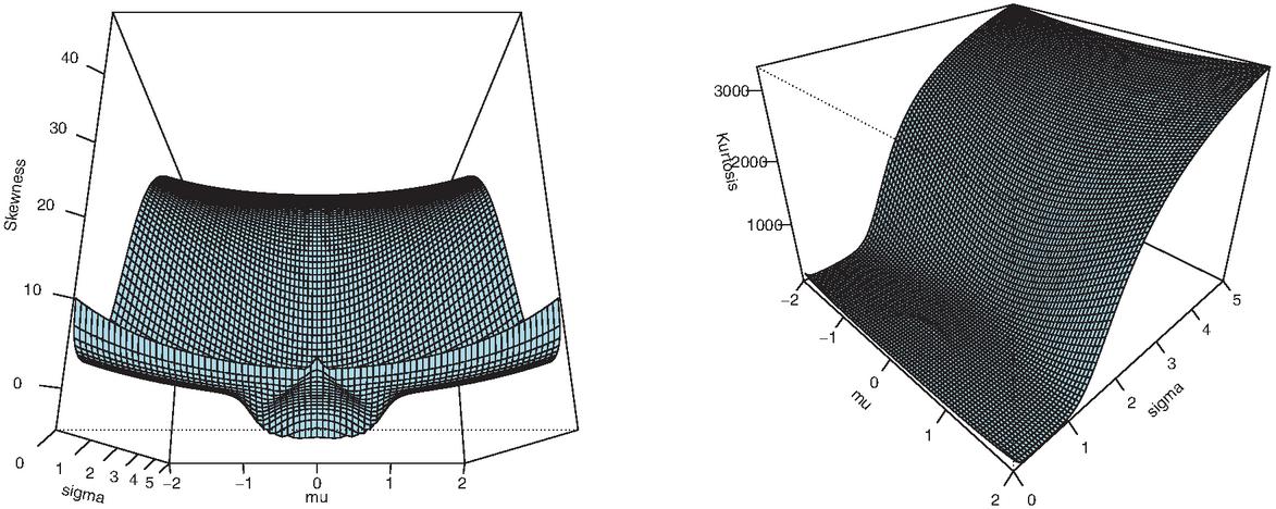
Figure 2 Three-dimensional plots of $S$ and $K$ for some ranges of parameter values.

From Figure 2, a great numerical versatility is observed for the considered skewness and kurtosis measures, depending on the values of $\mu$ and $\sigma$. This is another modeling benefit to the credit of the $UFN$ distribution.

The incomplete moments of the $UFN$ distribution can be expressed in a similar manner. The corresponding result is formulated in the new proposition.

Proposition 3.

Firstly, let $U$ be a RV following the $N\mathit{}\mathrm{(}\mathrm{0}\mathrm{,}\mathrm{1}\mathrm{)}$ distribution. Then, we define the double truncated moment generating function of $U$ as $M_{a\mathrm{,}b}\mathrm{(}t\mathrm{)}\mathrm{=}E\mathrm{\left[}{e}^{t\mathit{}U}I\mathrm{(}a\mathrm{<}U\mathrm{<}b\mathrm{)}\mathrm{\right]}$, $t\mathrm{,}a\mathrm{\in }\mathrm{R}$ and $b\mathrm{\in }\mathrm{(}a\mathrm{,}\mathrm{+}\mathrm{\infty }\mathrm{)}$. Now, let $m$ be a positive integer and $X\mathrm{\sim }U\mathit{}F\mathit{}N\mathit{}\mathrm{(}\mu \mathrm{,}\sigma \mathrm{)}$. Then, the $m$-th incomplete moment of $X$ depending on $u\mathrm{\in }\mathrm{(}\mathrm{0}\mathrm{,}\mathrm{1}\mathrm{)}$ can be expressed as

${\theta }_m(u)$	$=E\left[X^{m}I(X\le u)\right]$
	$={\displaystyle \sum _{k=0}^m}{\displaystyle \sum _{\mathrm{\ell }=0}^{+\mathrm{\infty }}}\left({\displaystyle \genfrac{}{}{0pt}{}{m}{k}}\right)\left({\displaystyle \genfrac{}{}{0pt}{}{-k}{\mathrm{\ell }}}\right){(-1)}^k{2}^k$
	$\mathrm{\hspace{1em}}\times [e^{-2(k+\mathrm{\ell })\mu }{M}_{-\frac{\mu }{\sigma },\frac{\mathrm{arctanh}(u)-\mu }{\sigma }}(-2(k+\mathrm{\ell })\sigma )$
	$\mathrm{\hspace{1em}}+e^{2\mathrm{\ell }\mu }{M}_{\frac{\mu }{\sigma },\frac{\mathrm{arctanh}(u)+\mu }{\sigma }}(-2\mathrm{\ell }\sigma )].$

The proof of Proposition 3 is similar to the proof of Proposition 2, we thus omit it. When $u$ tends to $1$, Proposition 3 becomes Proposition 2.

Taking $m=1$ yields the first incomplete moment, ${\theta }_1(u)$. It is especially useful for calculating the Bonferroni and Lorenz curves, moments of the standard and reversed residual life, and mean deviations for the $UFN$ distribution. All of them can be evaluated numerically.

3.5 Order Statistics

The minimal theory on the distributions of order statistics is described below. First, let $(X_1,X_2,\mathrm{\dots },X_n)$ be a $n$-random sample from the $UFN$ distribution. Then, by placing them in ascending order, we define the order statistics denoted by $X_{(1)},X_{(2)},\mathrm{\dots },X_{(n)}$. Then, for $i=1,2,\mathrm{\dots },n$, the PDF of $X_{(i)}$ is specified by

$$f_{X_{(i)}}(x,\mu ,\sigma )=C_{i,n}{[F(x,\mu ,\sigma )]}^{i-1}{[1-F(x,\mu ,\sigma )]}^{n-i}f(x,\mu ,\sigma ),$$

(6)

where $C_{i,n}=n!/[(i-1)!(n-i)!]$.

Explicitly, by using Equations (1) and (1), for $x\in (0,1)$, we get

$f_{X_{(i)}}(x,\mu ,\sigma )$	$=C_{i,n}{\displaystyle \frac{1}{\sigma (1-x^2)}}\left[\varphi \left({\displaystyle \frac{\mathrm{arctanh}x+\mu }{\sigma }}\right)+\varphi \left({\displaystyle \frac{\mathrm{arctanh}x-\mu }{\sigma }}\right)\right]$
	$\mathrm{\hspace{1em}}\times {\left[\mathrm{\Phi }\left({\displaystyle \frac{\mathrm{arctanh}x+\mu }{\sigma }}\right)+\mathrm{\Phi }\left({\displaystyle \frac{\mathrm{arctanh}x-\mu }{\sigma }}\right)-1\right]}^{i-1}$
	$\mathrm{\hspace{1em}}\times {\left[2-\mathrm{\Phi }\left({\displaystyle \frac{\mathrm{arctanh}x+\mu }{\sigma }}\right)-\mathrm{\Phi }\left({\displaystyle \frac{\mathrm{arctanh}x-\mu }{\sigma }}\right)\right]}^{n-i}.$

For $x\notin (0,1)$, we apply the standard completions on this function. In particular, by taking $i=n$, for $x\in (0,1)$, the maximum RV $X_{(n)}$ has the following PDF:

$f_{X_{(n)}}(x,\mu ,\sigma )$	$=n{\displaystyle \frac{1}{\sigma (1-x^2)}}\left[\varphi \left({\displaystyle \frac{\mathrm{arctanh}x+\mu }{\sigma }}\right)+\varphi \left({\displaystyle \frac{\mathrm{arctanh}x-\mu }{\sigma }}\right)\right]$
	$\mathrm{\hspace{1em}}\times {\left[\mathrm{\Phi }\left({\displaystyle \frac{\mathrm{arctanh}x+\mu }{\sigma }}\right)+\mathrm{\Phi }\left({\displaystyle \frac{\mathrm{arctanh}x-\mu }{\sigma }}\right)-1\right]}^{n-1}.$

Also, by taking $i=1$, for $x\in (0,1)$, the minimum RV $X_{(1)}$ has the following PDF:

$f_{X_{(1)}}(x,\mu ,\sigma )$	$=n{\displaystyle \frac{1}{\sigma \left(1-x^2\right)}}\left[\varphi \left({\displaystyle \frac{\mathrm{arctanh}x+\mu }{\sigma }}\right)+\varphi \left({\displaystyle \frac{\mathrm{arctanh}x-\mu }{\sigma }}\right)\right]$
	$\times {\left[2-\mathrm{\Phi }\left({\displaystyle \frac{\mathrm{arctanh}x+\mu }{\sigma }}\right)-\mathrm{\Phi }\left({\displaystyle \frac{\mathrm{arctanh}x-\mu }{\sigma }}\right)\right]}^{n-1}.$

Order statistics are the main ingredients of useful estimation methods. Some of them will be described in the next estimation study.

4 Estimation Methods

Here, we present six different methods that are useful to estimate the parameters of the $UFN$ distribution. The methods are supported by simulation studies.

4.1 Maximum Likelihood Method

Here, the estimation of the parameters is examined via the well-established method of maximum likelihood (ML) method. Let $(X_1,X_2,\mathrm{\dots },X_n)$ be a $n$-random sample from the $UFN$ distribution. The observed values are classically denoted by $x_1,x_2,\mathrm{\dots },x_n$, referring to generic data, and the model parameter vector is specified as $\mathbf{\Xi }={(\mu ,\sigma )}^T$. Then, the log-likelihood function is given as

$\mathrm{\ell }=\mathrm{\ell }\left(\mathbf{\Xi }\right)$	$=-n\log \sigma -{\displaystyle \frac{n}{2}}\log \left(2\pi \right)-{\displaystyle \sum _{i=1}^n}\log \left(1-x_i^2\right)$
	$\mathrm{\hspace{1em}}-{\displaystyle \frac{1}{2{\sigma }^2}}{\displaystyle \sum _{i=1}^n}{\left(\mathrm{arctanh}(x_i)-\mu \right)}^2$
	$\mathrm{\hspace{1em}}+{\displaystyle \sum _{i=1}^n}\log \left[1+e^{-\frac{2\mu }{{\sigma }^2}\mathrm{arctanh}(x_i)}\right].$	(7)

Following normal routine, the ML estimates (MLEs) ${\widehat{\mu }}_{MLE}$ and ${\widehat{\sigma }}_{MLE}$ of $\mu$ and $\sigma$, respectively, can be derived by maximizing $\mathrm{\ell }\left(\mathbf{\Xi }\right)$ with respect to $\mathbf{\Xi }$, also being the solutions of the following equations:

${\displaystyle \frac{\partial \mathrm{\ell }(\mathbf{\Xi })}{\partial \mu }}$	$={\displaystyle \frac{1}{{\sigma }^2}}{\displaystyle \sum _{i=1}^n}\left(\mathrm{arctanh}(x_i)-\mu \right)$
	$\mathrm{\hspace{1em}}-{\displaystyle \frac{2}{{\sigma }^2}}{\displaystyle \sum _{i=1}^n}{\displaystyle \frac{\mathrm{arctanh}(x_i)e^{-\frac{2\mu }{{\sigma }^2}\mathrm{arctanh}(x_i)}}{1+e^{-\frac{2\mu }{{\sigma }^2}\mathrm{arctanh}(x_i)}}}=0$	(8)

and

${\displaystyle \frac{\partial \mathrm{\ell }(\mathbf{\Xi })}{\partial \sigma }}$	$=-{\displaystyle \frac{n}{\sigma }}+{\displaystyle \frac{1}{{\sigma }^3}}{\displaystyle \sum _{i=1}^n}{\left(\mathrm{arctanh}(x_i)-\mu \right)}^2$
	$\mathrm{\hspace{1em}}+{\displaystyle \frac{4\mu }{{\sigma }^3}}{\displaystyle \sum _{i=1}^n}{\displaystyle \frac{\mathrm{arctanh}(x_i)e^{-\frac{2\mu }{{\sigma }^2}\mathrm{arctanh}(x_i)}}{1+e^{-\frac{2\mu }{{\sigma }^2}\mathrm{arctanh}(x_i)}}}=0.$	(9)

From Equation (4.1), we have

${\displaystyle \frac{1}{2}}{\displaystyle \sum _{i=1}^n}\left(\mathrm{arctanh}(x_i)-\mu \right)={\displaystyle \sum _{i=1}^n}{\displaystyle \frac{\mathrm{arctanh}(x_i)e^{-\frac{2\mu }{{\sigma }^2}\mathrm{arctanh}(x_i)}}{1+e^{-\frac{2\mu }{{\sigma }^2}\mathrm{arctanh}(x_i)}}}.$

Based on Equations (4.1) and (4.1), the following equation is obtained:

${\sigma }^2$	$={\displaystyle \frac{1}{n}}\left[{\displaystyle \sum _{i=1}^n}{\left(\mathrm{arctanh}(x_i)-\mu \right)}^2+2\mu {\displaystyle \sum _{i=1}^n}\left(\mathrm{arctanh}(x_i)-\mu \right)\right]$
	$={\displaystyle \frac{1}{n}}{\displaystyle \sum _{i=1}^n}{\left(\mathrm{arctanh}(x_i)\right)}^2-{\mu }^2.$	(11)

Then, putting Equation (4.1) into Equation (4.1), the profile log-likelihood with respect to $\mu$ is specified as

$\mathrm{\ell }\left(\mu \right)$	$=-{\displaystyle \frac{n}{2}}\log \left[{\displaystyle \frac{1}{n}}{\displaystyle \sum _{i=1}^n}{\left(\mathrm{arctanh}(x_i)\right)}^2-{\mu }^2\right]-{\displaystyle \frac{n}{2}}\log \left(2\pi \right)$
	$\mathrm{\hspace{1em}}-{\displaystyle \sum _{i=1}^n}\log \left(1-x_i^2\right)-{\displaystyle \frac{\sum _{i=1}^n{\left(\mathrm{arctanh}(x_i)-\mu \right)}^2}{2\left(\frac{1}{n}\sum _{i=1}^n{\left(\mathrm{arctanh}(x_i)\right)}^2-{\mu }^2\right)}}+{\displaystyle \sum _{i=1}^n}\log$
	$\mathrm{\hspace{1em}}\left[1+\exp \left\{-2\mu \mathrm{arctanh}(x_i){\left({\displaystyle \frac{1}{n}}{\displaystyle \sum _{i=1}^n}{\left(\mathrm{arctanh}(x_i)\right)}^2-{\mu }^2\right)}^{-1}\right\}\right].$

It satisfies

${\displaystyle \frac{\partial \mathrm{\ell }\left(\mu \right)}{\partial \mu }}$	$={\displaystyle \frac{n\mu }{\frac{1}{n}\sum _{i=1}^n{\left(\mathrm{arctanh}\left(x_i\right)\right)}^2-{\mu }^2}}$
	$\mathrm{\hspace{1em}}-{\displaystyle \frac{\begin{array}{c}\mu \sum _{i=1}^n{\left(\mathrm{arctanh}\left(x_i\right)-\mu \right)}^2\hfill \\ -\sum _{i=1}^n\left(\mathrm{arctanh}\left(x_i\right)-\mu \right)\left(\frac{1}{n}\sum _{i=1}^n{\left(\mathrm{arctanh}\left(x_i\right)\right)}^2-{\mu }^2\right)\hfill \end{array}}{{\left(\frac{1}{n}\sum _{i=1}^n{\left(\mathrm{arctanh}\left(x_i\right)\right)}^2-{\mu }^2\right)}^2}}$
	$\mathrm{\hspace{1em}}-{\displaystyle \sum _{i=1}^n}{\displaystyle \frac{\begin{array}{c}2\mathrm{arctanh}\left(x_i\right)\left(\frac{1}{n}\sum _{i=1}^n{\left(\mathrm{arctanh}\left(x_i\right)\right)}^2+4{\mu }^2\right)\exp \hfill \\ \left\{-2\mu \mathrm{arctanh}\left(x_i\right){\left(\frac{1}{n}\sum _{i=1}^n{\left(\mathrm{arctanh}\left(x_i\right)\right)}^2-{\mu }^2\right)}^{-1}\right\}\hfill \end{array}}{\begin{array}{c}{\left(\frac{1}{n}\sum _{i=1}^n{\left(\mathrm{arctanh}\left(x_i\right)\right)}^2-{\mu }^2\right)}^2\hfill \\ \left(1+\exp \left\{-2\mu \mathrm{arctanh}\left(x_i\right){\left(\frac{1}{n}\sum _{i=1}^n{\left(\mathrm{arctanh}\left(x_i\right)\right)}^2-{\mu }^2\right)}^{-1}\right\}\right)\hfill \end{array}}}.$

Hence, we need to solve the following equation: $\partial \mathrm{\ell }\left(\mu \right)/(\partial \mu )=0$; numerical techniques are needed to get the ${\widehat{\mu }}_{MLE}$. After obtaining the ${\widehat{\mu }}_{MLE}$, the ${\widehat{\sigma }}_{MLE}$ is determined by taking the square root of ${\widehat{\sigma }}_{MLE}^2$ as defined in Equation (4.1) with $\mu ={\widehat{\mu }}_{MLE}$.

For the interval estimations of the parameters $\mu$ and $\sigma$, the observed information matrix is required. Here, this matrix is defined by

$$I={\left(\begin{array}{cccccccccccccccccccc}\hfill -\frac{{\partial }^2\mathrm{\ell }\left(\mathbf{\Xi }\right)}{\partial {\mu }^2}\hfill & \hfill -\frac{{\partial }^2\mathrm{\ell }\left(\mathbf{\Xi }\right)}{\partial \mu \partial \sigma }\hfill & & & & & & & & & & & & & & & & & & \\ \hfill -\frac{{\partial }^2\mathrm{\ell }\left(\mathbf{\Xi }\right)}{\partial \sigma \partial \mu }\hfill & \hfill -\frac{{\partial }^2\mathrm{\ell }\left(\mathbf{\Xi }\right)}{\partial {\sigma }^2}\hfill & & & & & & & & & & & & & & & & & & \end{array}\right)|}_{\mu ={\widehat{\mu }}_{MLE},\sigma ={\widehat{\sigma }}_{MLE}}.$$

Under mild conditions identified as ‘regularity conditions’, one can use the two-dimensional normal distribution with mean vector $\mathbf{\Xi }$ and covariance matrix $I^{-1}$ for interval estimations. The formulas for the components of $I$ are available upon author request. Several alternative methods to the ML method have been proposed. Some of them are briefly presented below.

4.2 Some Other Estimation Methods

Maximum product spacing (MPS) method

First, the MPS method was developed by [9] and [40]. It can be described as follows. Let $x_{(1)},x_{(2)},\mathrm{\dots },x_{(n)}$ be $x_1,x_2,\mathrm{\dots },x_n$ put in an ascending order. Let us set

$$GM(\mathbf{\Xi })=\sqrt[n+1]{\prod _{i=1}^{n+1}\left[F(x_{(i)},\mu ,\sigma )-F(x_{(i-1)},\mu ,\sigma )\right]},$$

with the conventions: $F(x_{(0)},\mu ,\sigma )=0$ and $F(x_{(n+1)},\mu ,\sigma )=1$. The MPS estimates (MPSEs) ${\widehat{\mu }}_{MPS}$ and ${\widehat{\sigma }}_{MPS}$ of $\mu$ and $\sigma$, respectively, are determined by maximizing $GM(\mathbf{\Xi })$ with respect to $\mathbf{\Xi }$.

Least square (LS) method

The LS estimates (LSEs) ${\widehat{\mu }}_{LSE}$ and ${\widehat{\sigma }}_{LSE}$ of the parameters $\mu$ and $\sigma$, respectively, are given by minimizing

$$LSE(\mathbf{\Xi })=\sum _{i=1}^n{\left(F(x_{(i)},\mu ,\sigma )-\frac{i}{n+1}\right)}^2,$$

with respect to $\mathbf{\Xi }$.

Weighted least square (WLS) method

In a similar way, the WLS estimates (WLSEs) ${\widehat{\mu }}_{WLSE}$ and ${\widehat{\sigma }}_{WLSE}$ of the parameters $\mu$ and $\sigma$, respectively, are determined by minimizing

$$WLSE(\mathbf{\Xi })=\sum _{i=1}^n{w}_{i,n}{\left(F(x_{(i)},\mu ,\sigma )-\frac{i}{n+1}\right)}^2,$$

with respect to $\mathbf{\Xi }$, where $w_{i,n}=[(n+2){(n+1)}^2]/i(n-i+1)$ for $i=1,2,\mathrm{\dots },n$.

Anderson-Darling (AD) method

The AD estimates (ADEs) ${\widehat{\mu }}_{AD}$ and ${\widehat{\sigma }}_{AD}$ of the parameters $\mu$ and $\sigma$, respectively, are got by minimizing

$AD\left(\mathbf{\Xi }\right)$	$=-n-{\displaystyle \sum _{i=1}^n}{\displaystyle \frac{2i-1}{n}}$
	$\mathrm{\hspace{1em}}\times \left[\log \left\{1-F(x_{(n+1-i)},\mu ,\sigma )+\log F(x_{(i)},\mu ,\sigma )\right\}\right],$

with respect to $\mathbf{\Xi }$.

Cramér-von Mises (CVM) method

The CVM estimates (CVMEs) ${\widehat{\mu }}_{CVM}$ and ${\widehat{\sigma }}_{CVM}$ of the parameters $\mu$ and $\sigma$, respectively, are acquired by minimizing

$$CVM\left(\mathbf{\Xi }\right)=\frac{1}{12n}+\sum _{i=1}^n{\left[F(x_{(i)},\mu ,\sigma )-\frac{2i-1}{2n}\right]}^2,$$

with respect to $\mathbf{\Xi }$.

4.3 Simulation Experiments

We now perform a simulation work based on $n$-random samples to evaluate the performance of the estimates presented above with respect to varying $n$. First, we generate $N=1000$ samples of size $n=20+5k$ with $k=0,1,\mathrm{\dots },196$ from the $UFN$ distribution. More precisely, we conducted two simulation studies where

• we take $\mu =1$, $\sigma =0.5$ and $\mu =2$, $\sigma =2$ for the first and second ones, respectively,

• the generated values are given by the formula $x=\left|\tanh y\right|$, where the $y$ is the random number from the $N(\mu ,{\sigma }^2)$ distribution.

The constrOptim routine available in the R program is employed. Further, we compute the average of the estimates (AEs), biases and mean square errors (MSE). Mathematically, for $h=\mu$ and $h=\sigma$, the AEs, biases and MSEs are calculated by

$A{E}_h(n)$	$=$	${\displaystyle \frac{1}{N}}{\displaystyle \sum _{i=1}^N}{\widehat{h}}_i,Bia{s}_h(n)=h-A{E}_h(n),$
$MS{E}_h(n)$	$=$	${\displaystyle \frac{1}{N}}{\displaystyle \sum _{i=1}^N}{(h-{\widehat{h}}_i)}^2,$

respectively, where the index $i$ refers to the $i$-th sample. We anticipate that the AEs are close to true values, especially when the biases and MSEs are almost zero. Figures 3 and 4 display the results of these two simulation studies.

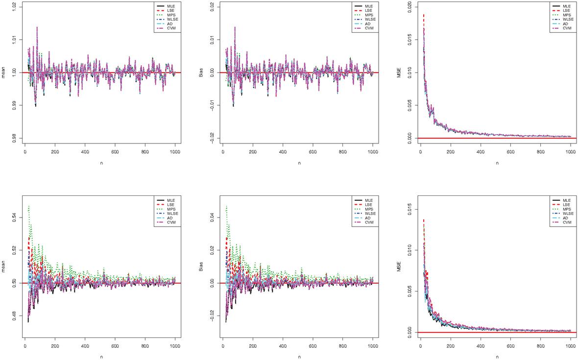
Figure 3 Graphical results of the $\mu$ (top) and $\sigma$ (bottom) parameters for the first simulation study.

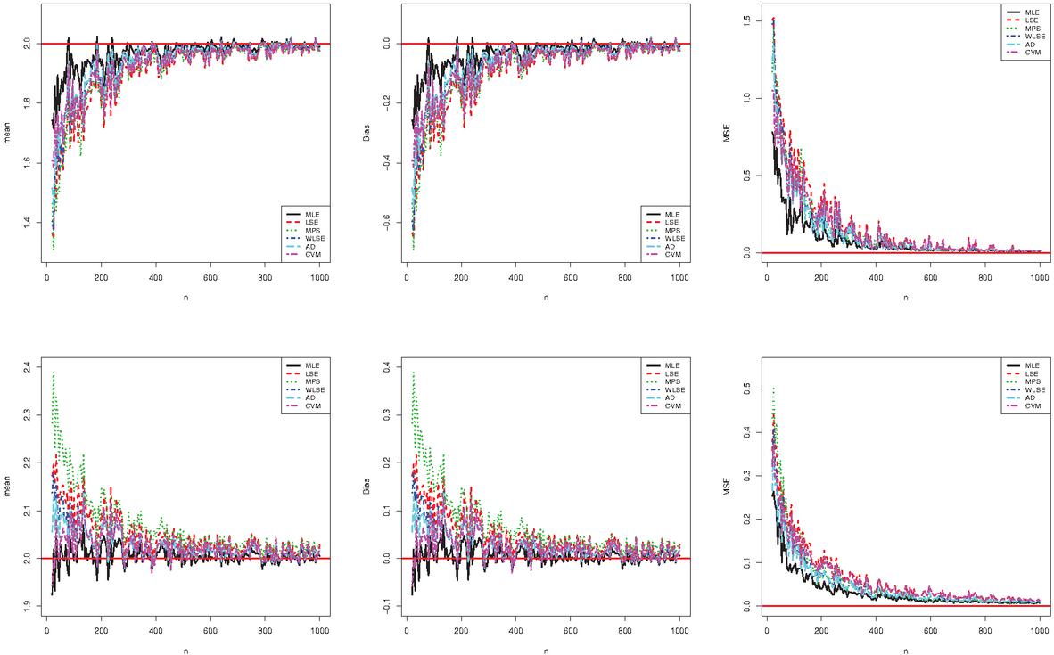
Figure 4 Graphical results of the $\mu$ (top) and $\sigma$ (bottom) parameters for the second simulation study.

Figures 3 and 4 illustrate the consistency of the estimates. In particular, the biases and MSEs decrease to zero when $n$ increases, as expected. Also, their unbiasedness is observed. The amount of biases and MSEs on changing sample size is very close to the parameter $\mu$, according to the first simulation study. In addition, the amount of the biases and MSEs of the MPS and LSE methods is the greatest initially for the parameter $\sigma$ according to changes in the sample size. However, when the sample size increases, these amounts are close together. According to the second simulation study, when changing sample size, the amount of bias and MSEs introduced by the ML method is the smallest for both parameters. However, when the sample size increases, these amounts are close together. Generally, the performance of all estimates is close. Similar simulation results can also be obtained for arbitrary parameter settings.

5 The Derived Quantile Regression Model

5.1 Description

If the response variable support is set to a unit interval, the use of a unit regression model based on the unit distribution is suitable to model the conditional mean of the response variable via independent variables (covariates). In this regard, Reference [12] proposed the beta regression model. For accurate model inference, when the response variable has outliers in the measures, robust estimation results based on the regression model are required. For this aim, the QR model is a solid alternative model to the ordinary LSE and beta regression models. Whereas the method of least squares and beta regression models estimate the conditional mean of the response variable, the QR estimates the conditional median or other quantiles of the response variable.

With this approach, [37] and [35] have introduced the Kumaraswamy and unit Weibull QR models by re-parametrization of the Kumaraswamy and unit Weibull models, respectively.

Now, we introduce an alternative QR model based on a special $UFN(\mu ,\sigma )$ distribution. In order to simplify the expression of the QF of the $UFN$ distribution, an exponentiated distribution version based on a special $UFN$ distribution is prefered. We call it as exponentiated $UFN$ ($EUFN$) distribution. Its CDF and PDF are listed by

$G(y,\alpha ,\sigma )={\left[F(y,0,\sigma )\right]}^{\alpha }={\left[2\mathrm{\Phi }\left({\displaystyle \frac{\mathrm{arctanh}y}{\sigma }}\right)-1\right]}^{\alpha }$

(12)

and

$g(y,\alpha ,\sigma )={\displaystyle \frac{2\alpha }{\sigma \left(1-y^2\right)}}\varphi \left({\displaystyle \frac{\mathrm{arctanh}y}{\sigma }}\right){\left[2\mathrm{\Phi }\left({\displaystyle \frac{\mathrm{arctanh}y}{\sigma }}\right)-1\right]}^{\alpha -1},$

respectively, where $y\in (0,1)$ and $\alpha ,\sigma >0$.

The QF of the $EUFN$ distribution is obtained by

$$Q(u,\alpha ,\sigma )=\tanh \left[\sigma {\mathrm{\Phi }}^{-1}\left(\frac{1+u^{\frac{1}{\alpha }}}{2}\right)\right],$$

where $u\in (0,1)$. Then, the PDF of the $EUFN$ distribution can be modified by putting $\eta =Q(u,\alpha ,\sigma )$. Thus, by setting $\sigma =\mathrm{arctanh}\eta /{\mathrm{\Phi }}^{-1}\left[(1+u^{\frac{1}{\alpha }})/2\right]$, the PDF of the modified distribution is given by

$g(y,\alpha ,\eta )$	$={\displaystyle \frac{2\alpha {\mathrm{\Phi }}^{-1}\left(\frac{1+u^{\frac{1}{\alpha }}}{2}\right)}{\mathrm{arctanh}\eta \left(1-y^2\right)}}$
	$\mathrm{\hspace{1em}}\times \varphi \left({\displaystyle \frac{\mathrm{arctanh}y}{\mathrm{arctanh}\eta }}{\mathrm{\Phi }}^{-1}\left({\displaystyle \frac{1+u^{\frac{1}{\alpha }}}{2}}\right)\right)$
	$\mathrm{\hspace{1em}}\times {\left[2\mathrm{\Phi }\left({\displaystyle \frac{\mathrm{arctanh}y}{\mathrm{arctanh}\eta }}{\mathrm{\Phi }}^{-1}\left({\displaystyle \frac{1+u^{\frac{1}{\alpha }}}{2}}\right)\right)-1\right]}^{\alpha -1},$	(13)

where $\eta$ is the quantile parameter. In this context, $u$ is a tuning parameter which is assumed to be known. We denote the distribution associated to Equation (13) with $EUFN(\alpha ,\eta ,u)$. Samples of the shapes of $g(y,\alpha ,\eta )$ are presented in Figure 5.

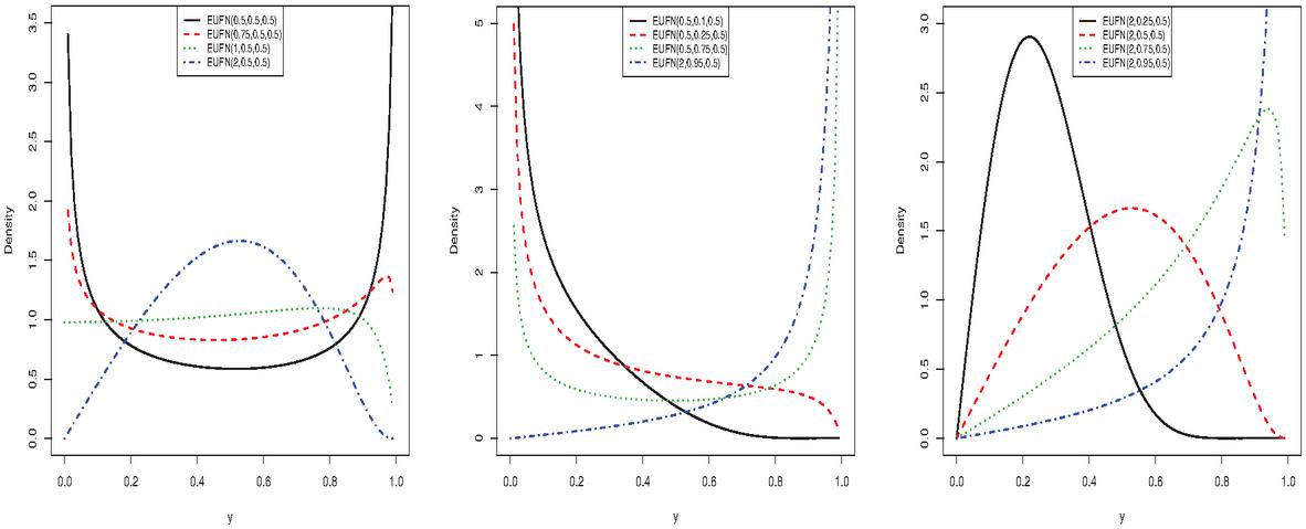
Figure 5 Samples of the PDF shapes of the modified $EUFN$ distribution.

We see that the $EUFN$ distribution has the skewed shapes as well as bathtub shaped, inverse N-shaped, decreasing, increasing and unimodal. The modelling of the conditional median follows by taking $u=0.5$.

We now present the QR model based on the $EUFN$ distribution with the PDF in Equation (13). In this regard, we consider $n$ observations $y_1,y_2,\mathrm{\dots },y_n$ from the re-parameterized $EUFN$ distribution such that $y_i$ is a realization of $Y_i\sim EUFN(\alpha ,{\eta }_i,u)$, with unknown parameters ${\eta }_i$ and $\beta$. Note that the parameter $u$ is known. The $EUFN$ QR model is defined as

$$g({\eta }_i)={\mathbf{x}}_i{\mathit{\beta }}^T,$$

where $\mathit{\beta }={({\beta }_0,{\beta }_1,{\beta }_2,\mathrm{\dots },{\beta }_p)}^T$ and ${\mathbf{x}}_i=(1,x_{i1},x_{i2},x_{i3},\mathrm{\dots },x_{ip})$are the unknown regression parameter vector and $i$ -th vector known to covariates. Thus defined, $g(x)$ is the link function which is used to relate the covariates at the conditional quantile of the response variable. For example, when $u=0.5$, the covariates are related to the conditional median of the response variable. Since the $EUFN$ distribution is set to the unit interval, we adopt the logit-link function such that

$$g({\eta }_i)=\log \left(\frac{{\eta }_i}{1-{\eta }_i}\right).$$

5.2 Parameter Estimation via the ML Method

Classically, the unknown parameters involved in the $EUFN$ QR model are estimated by the ML method. Consider the link function below:

$$g({\eta }_i)=\log \left(\frac{{\eta }_i}{1-{\eta }_i}\right)={\mathbf{x}}_i{\mathit{\beta }}^T.$$

(14)

From Equation (14), it comes

$${\eta }_i=\frac{\exp \left({\mathbf{x}}_i{\mathit{\beta }}^T\right)}{1+\exp \left({\mathbf{x}}_i{\mathit{\beta }}^T\right)}.$$

(15)

Let $\mathbf{\Omega }={(\alpha ,\mathit{\beta })}^T$ be the unknown parameter vector. Then, inserting Equation (15) in Equation (13), the log-likelihood function of the $EUFN$ QR model is

$\mathrm{\ell }\left(\mathbf{\Omega }\right)$	$=n\log 2-{\displaystyle \frac{n}{2}}\log \left(2\pi \right)+n\log \alpha$
	$\mathrm{\hspace{1em}}+n\log \left[{\mathrm{\Phi }}^{-1}\left({\displaystyle \frac{1+u^{\frac{1}{\alpha }}}{2}}\right)\right]-{\displaystyle \sum _{i=1}^n}\log \left[\mathrm{arctanh}({\eta }_i)\left(1-y_i^2\right)\right]$
	$\mathrm{\hspace{1em}}-{\displaystyle \frac{1}{2}}{\left[{\mathrm{\Phi }}^{-1}\left({\displaystyle \frac{1+u^{\frac{1}{\alpha }}}{2}}\right)\right]}^2{\displaystyle \sum _{i=1}^n}{\left({\displaystyle \frac{\mathrm{arctanh}(y_i)}{\mathrm{arctanh}({\eta }_i)}}\right)}^2$
	$\mathrm{\hspace{1em}}+(\alpha -1){\displaystyle \sum _{i=1}^n}\log \left[2\mathrm{\Phi }\left({\displaystyle \frac{\mathrm{arctanh}(y_i)}{\mathrm{arctanh}({\eta }_i)}}{\mathrm{\Phi }}^{-1}\left({\displaystyle \frac{1+u^{\frac{1}{\alpha }}}{2}}\right)\right)-1\right].$	(16)

Since Equation (16) is composed of nonlinear functions according to the parameters of the model, this log-likelihood function can be maximized automatically by software such as R, Python, Matlab and Mathematica. We thus obtain the MLE denoted by $\widehat{\mathbf{\Omega }}={(\widehat{\alpha },\widehat{\mathit{\beta }})}^T$. Here, we employ the maxLik function [23] of the R software to maximize Equation (16). This function also gives the components of the observed information matrix, including the standard errors (SEs). Recent advances in QR modelling with the ML method can be found in [24, 15, 31, 35] and [29].

5.3 Analysis of the Residuals for the Model Checking

Residual analysis may be necessary to verify if the regression model is appropriate. To see this, a residual analysis can be performed. Here, we indicate the randomized quantile and the Cox-Snell residuals.

Randomized quantile residuals

The randomized quantile residuals have been introduced by [11]. The $i$-th randomized quantile residual is determined as

$${\widehat{r}}_i={\mathrm{\Phi }}^{-1}\left[G(y_i,\widehat{\alpha },\widehat{{\eta }_i})\right]$$

for $i=1,\mathrm{\dots },n$, where $G(y,\alpha ,\eta )$ is the CDF of the modified $EUFN$ distribution and ${\widehat{\eta }}_i$ is defined by Equation (15) with $\mathit{\beta }$ estimated by $\widehat{\mathit{\beta }}$. If the fitted model successfully processes the data set, the underlying distribution of a randomized quantile residual corresponds to the $N(0,1)$ distribution.

Cox-Snell residuals

Alternatively, one can consider the Cox and Snell residuals developed by [10]. The $i$-th Cox-Snell residual is given by

$${\widehat{e}}_i=-\log \left[1-G(y_i,\widehat{\alpha },\widehat{{\eta }_i})\right]$$

for $i=1,\mathrm{\dots },n$. If the model fits to data suitably, the distribution of a Cox-Snell residual corresponds to the standard exponential distribution.

6 Data Analysis

In this section, two data applications have been given to see applicability of the proposed distribution model.

6.1 Description

We obtain all the data sets from OECD.Stat with the following uniform resource locator: https://stats.oecd.org/. It includes data and metadata for the OECD countries and selected non-member economies. The OECD.Stat consists of crucial themes such as Agriculture and Fisheries, Demography, Education and Training, Labour, Health, Social Protection, Finance, and Well-being, etc. Each theme is divided into various areas. Here, we consider the BLI of both OECD countries and some non-economy OECD countries in the Social Protection and Well-being theme. For the analysis of the two data, the educational attainment values are used as an indicator in the education theme of the BLI. The dataset used covers educational attainment values for OECD countries as well as for Brazil, Russia and South Africa. The percentage is the unit of measurement. The first application is about univariate modeling of educational attainment for the $UFN$ distribution. The second application is about the QR modeling for the $EUFN$ distribution to relate educational attainment of the above countries with some indicators of topics of BLIs such as work-life balance, safety, and health. The reference year of the indicators is 2017. The data set can be directly found in https://stats.oecd.org/index.aspx?DataSetCode=BLI.

6.2 Univariate Data Modeling

Here, a real data set is analyzed to prove the empirical importance and modeling ability of the proposed $UFN$ model. This data set has been examined by [4] for another unit distribution, which is called the log-weighted exponential distribution. The author has obtained the estimated log-likelihood, denoted by $\widehat{\mathrm{\ell }}$, value of $24.8655$ for his model.

Figure 6 displays the boxplot of the data set.

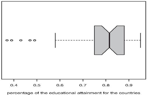
Figure 6 Boxplot of the considered data set.

From Figure 6, it appears that the data set is left skewed and it has some outliers.

We compare the performance of the real data fitting of the $UFN$ distribution through the ML method with the following well-established unit distributions:

• Beta distribution:

$$f_{Beta}(x,\mu ,\sigma )=\frac{1}{\mathrm{B}(\mu ,\sigma )}{x}^{\mu -1}{\left(1-x\right)}^{\sigma -1},$$

where $x\in (0,1)$, $\mu >0$, $\sigma >0$, and $\mathrm{B}(\mu ,\sigma )$ is the beta function.

• Johnson $S_B$ distribution:

$$f_{S_B}(x,\mu ,\sigma )=\frac{\sigma }{x\left(1-x\right)}\varphi \left[\sigma \log \left(\frac{x}{1-x}\right)+\mu \right],$$

where $x\in (0,1)$, $\mu \in ℝ$ and $\sigma >0$. We note that the density $f_{S_B}(x,-\mu /\sigma ,1/\sigma )$ is known as the PDF of the logit normal distribution.

• Exponentiated Topp Leone (ETL) distribution (see [39]:

$$f_{ETL}(x,\mu ,\sigma )=2\sigma \mu {\left[x\left(2-x\right)\right]}^{\mu -1}\left(1-x\right){\left\{1-{\left[x\left(2-x\right)\right]}^{\mu }\right\}}^{\sigma -1},$$

where $x\in (0,1)$, $\mu >0$ and $\sigma >0$.

• Kumaraswamy (Kw) distribution:

$$f_{Kw}(x,\mu ,\sigma )=\sigma \mu {\left(1-x^{\mu }\right)}^{\sigma -1}{x}^{\mu -1},$$

where $x\in (0,1)$, $\mu >0$ and $\sigma >0$.

• Unit generalized half normal (UGHN) distribution (see [27]):

$$f_{UGHN}(x,\mu ,\sigma )=\frac{2\mu {\left(-\log x\right)}^{\mu -1}}{x{\sigma }^{\mu }}\varphi \left[{\left(\frac{-\log x}{\sigma }\right)}^{\mu }\right],$$

where $x\in (0,1)$, $\mu >0$ and $\sigma >0$.

The $\widehat{\mathrm{\ell }}$ values, Akaike information criterion (AIC), Bayesian information criterion (BIC), Kolmogorov-Smirnov ($KS$), Cramér-von Mises ($W^{\ast }$) and Anderson-Darling ($A^{\ast }$) goodness of-fit statistics are obtained based on all distribution models to determine the optimum model. In general, one can choose as the optimal model the one indicating the smallest values of AIC, BIC, KS, $W^{\ast }$ and $A^{\ast }$ statistics, and the largest values of $\widehat{\mathrm{\ell }}$ and $KS$ p-value.

Firstly, we fit the folded normal ($FN$) distribution, which has the following PDF: $f_{FN}(x,\mu ,\sigma )=(1/\sigma )\left[\varphi \left((x+\mu )/\sigma \right)+\varphi \left((x-\mu )/\sigma \right)\right]$, $x>0$, $\mu \in ℝ$ and $\sigma >0$, to this data set. For this model, we obtained the $\widehat{\mathrm{\ell }}$ value and $KS$ statistics as $16.2354$ and 0.2309 (with p-value $=0.0348$), respectively. It is clear that the $FN$ model is inadequate for explaining to this data set. We give the data analysis results belong to other competitor models in Table 1.

Table 1 MLEs, SEs (in parentheses), $\widehat{\mathrm{\ell }}$ and goodness-of-fits statistics (the p-values of the KS test are given in $[\cdot ]$)

Model	$\widehat{\mu }$	$\widehat{\sigma }$	$\widehat{\mathrm{\ell }}$	$AIC$	$BIC$	$A^{*}$	$W^{*}$	$KS$
UFN	1.1302	0.3678	26.8429	$-$49.6858	$-$46.4106	0.4850	0.0736	0.1195
	(0.0597)	(0.0424)						[0.6502]
UGHN	0.9558	0.3698	20.2884	$-$36.5769	$-$33.3018	1.8384	0.3276	0.2097
	(0.1208)	(0.0498)						[0.0706]
Beta	5.9874	1.8157	23.8684	$-$43.7369	$-$40.4616	1.2732	0.2233	0.1826
	(1.7258)	(0.4566)						[0.1588]
Kw	5.4450	2.0847	24.3538	$-$44.7076	$-$41.4324	1.2057	0.2057	0.1740
	(1.0292)	0.5383						[0.2001]
ETL	8.5134	0.6642	22.0160	$-$40.0320	$-$36.7568	1.8182	0.3524	0.2198
	(2.0971)	(0.1354)						[0.0508]
Johnson $S_B$	$-$1.6045	1.1403	26.2280	$-$48.4560	$-$45.1809	0.7540	0.1229	0.1472
	(0.2455)	(0.1308)						[0.3828]

Table 1 reveals that the $UFN$ distribution has the lowest values of AIC and BIC statistics. Also, the $UFN$ distribution has the lowest values of the $A^{\ast }$ and $W^{\ast }$ and KS statistics with higher p-value. Hence, the $UFN$ distribution is the best choice for the modeling.

Figure 7 shows some important estimated functions of the $UFN$ distribution to graphically prove the fit of the model.

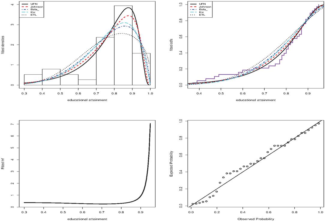
Figure 7 Some fitted functions for the used data.

Clearly, the proposed model has successfully captured the skewness and kurtosis of the data set. The plotted lines of the probability-probability (PP) plot is very closer the diagonal line which indicates that the performance of the $UFN$ distribution is acceptable for the modeled data. In order to show that the likelihood equations have a unique solution, we display the profile log-likelihood (PLL) functions of the parameters $\mu$ and $\sigma$ for the data set in Figure 8.

Figure 8 Plots of the PLL functions for the considered data set.

The maxima of the curves indicate that the likelihood equations have unique solutions for the MLEs.

6.3 QR Modeling for the Educational Attainment Data Set

In this section, a real application is provided in order to highlight the applicability of the newly defined QR model. Two important competitor regression models are considered. They are beta regression [12] model as well as Kumaraswamy QR [37] model. Their PDFs are

$$f_{Beta}(y,\alpha ,\eta )=\frac{\mathrm{\Gamma }\left(\alpha \right)}{\mathrm{\Gamma }\left(\alpha \eta \right)\mathrm{\Gamma }\left(\left(1-\eta \right)\alpha \right)}{y}^{\alpha \eta -1}{\left(1-y\right)}^{\left(1-\eta \right)\alpha -1},y\in (0,1),$$

where $\eta \in (0,1)$ is the mean and $\alpha >0$ and

$$f_{Kw}(y,\alpha ,\eta )=\frac{\alpha \log \left(0.5\right)}{\log \left(1-{\eta }^{\alpha }\right)}{\left(1-y^{\alpha }\right)}^{\log \left(0.5\right)/\left(\alpha \left(1-\eta \right)-1\right)}{y}^{\alpha -1},y\in (0,1),$$

where $\eta \in (0,1)$ is the median and $\alpha >0$ for the beta regression and Kumaraswamy QR, respectively.

Here, we want to relate the level of education of the countries with the variables of some BLIs such as work-life balance, safety, and health. In this context, the aim of this application is to linearly explain the educational attainment values $(y)$ with the percentage of the employees working very long hours $(x_1)$, homicide rate $(x_2)$, and self-reported health $(x_3)$ covariates. The values of these indicators belong to the OECD countries as well as Brazil, Russia, and South Africa. Specifically, $x_1$ is the proportion of dependent employees whose usual working hours per week are 50 hours or more, $x_2$ is the ratio of deaths due to assault as a standardized rate according to age per 100,000 population, and $x_3$ is the percentage of the population aged 15 and over who report good or better health. One may see the data set and detailed information about all covariates via the link which has been given in Section 6. The following linear regression equation is used for all the regression models:

$$\mathrm{logit}({\eta }_i)={\beta }_0+{\beta }_1{x}_{i1}+{\beta }_2{x}_{i2}+{\beta }_3{x}_{i3},i=1,2,\mathrm{\dots },38,$$

where the ${\eta }_i$ is the mean for the beta model whereas it denotes the median for the Kumaraswamy and $EUFN$ models.

From Figure 6, we see that the data are skewed and have some outliers. For these reasons, relating the unit response variable with covariates via the median QR will be more useful for the inferences, since the mean is perturbed by skewed data with the outliers precisely. Thus, it can be obtained as a more illustrative and more robust inference than the mean response regression.

We use the betareg function of the R software for the results of the beta regression model. The maxLik function [23] of the R software has been used for the results of the $EUFN$, Kumaraswamy, and unit-Weibull QR models. The details are given as follows.

Firstly, we assume that $u=0.5$ for the three QR models for the median modeling. The obtained results are contained in Table 2.

Table 2 Results of the fitted regression models with the considered model selection criteria

Parameters	Beta			Kumaraswamy			EUFN
	Estimate	SE	p-value	Estimate	SE	p-value	Estimate	SE	p-value
${\beta }_0$	2.5107	0.5606	$<0.001$	2.7648	0.4293	$<0.001$	2.9713	0.6000	$<0.001$
${\beta }_1$	$-$4.1441	1.2998	$0.0014$	$-$4.8408	1.1903	$<0.001$	$-$5.5763	1.4511	$<0.001$
${\beta }_2$	$-$0.0512	0.0176	$0.0036$	$-$0.0642	0.0105	$<0.001$	$-$0.0578	0.0173	$<0.001$
${\beta }_3$	$-$1.0869	0.7605	$0.1530$	$-$1.1092	0.5034	$0.0276$	$-$1.3746	0.7799	$0.0780$
$\alpha$	12.2220	2.7550	$<0.001$	6.8593	1.1576	$<0.001$	6.6951	1.7689	$<0.001$
$\widehat{\mathrm{\ell }}$	31.8600	31.8542	32.5631
AIC	$-$53.7200	$-$53.7083	$-$55.1263
BIC	$-$45.5321			$-$45.5204			$-$46.9384

From this table, the parameters ${\beta }_1$ and ${\beta }_2$ are seen as significant at any usual level, as well as the parameter ${\beta }_3$ is seen to be significant at an 8% level for the $EUFN$ regression model. For the Kumaraswamy regression model, all parameters are significant at any usual level.

According to our regression model, the unit median response variable is negatively affected by all the covariates. Hence, it can be concluded that in the related countries, when the percentage of employees working very long hours, the homicide rate, and the percentage of the population who report their health as good or better increase, the percentage of educational attainment decreases. The result of self-reported health according to educational attainment turns out out to be surprisingly surprising. It is obvious that all covariates affect educational attainment negatively. Moreover, in view of the AIC and BIC values, it can be concluded that the proposed regression model is the best.

To complete this work, the Quantile-Quantile (QQ) plots of the randomized quantile residuals and the PP plots of the Cox-Snell residuals for all the models are displayed in Figures 9 and 10, respectively.

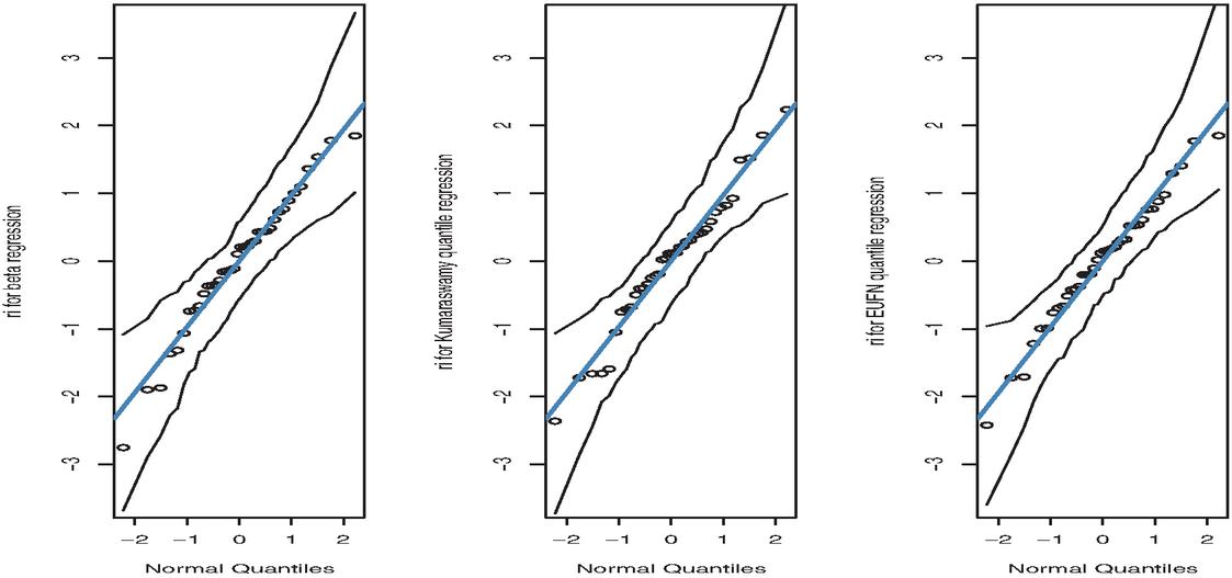
Figure 9 QQ plots of the randomized quantile residuals for the regression models.

Figure 10 PP plots of the Cox-Snell residuals for the regression models.

The plots of the $EUFN$ regression model are close to the diagonal line, as shown in Figures 9 and 10. Hence, the randomized quantile and Cox-Snell residuals based $EUFN$ regression model have the $N(0,1)$ and exponential distributions, respectively. Finally, we can say that the data set is modeled by the $EUFN$ regression model more successfully than the other models.

7 Conclusion

We motivate and study a new unit distribution, called the unit folded normal ($UFN$) distribution, to model the proportion of educational attainment and other data sets defined over the unit interval. We study the characteristics and properties of the new distribution. Six methods are used to estimate the model parameters. Two simulation studies were conducted to illustrate the performance of these estimates. The percentage of educational attainment data set of both OECD countries and some non-economy OECD countries is considered to point out the applicability of the $UFN$ distribution. The findings, which are about the modeling of educational attainment, show that the proposed model provides better fits than referenced unit models. According to its regression modeling, it also aimed to relate the educational attainment in the countries with their employees working very long hours, homicide rate, and self-reported health via median QR modeling. The results indicate important findings on how these covariates affect the unit response variable titled ”Country Educational Attainment.”

Most surprising is the finding that, according to the estimated regression coefficients, there is an inverse relationship between education level and self-reported health status, statistically significant at an 8% significance level. That is, the percentages of educational attainment in countries are influenced negatively by those of self-reported health.Hence, the result of self-reported health according to educational attainment turns out surprisingly. Based on the dataset from 69 countries, [43] have shown that adults with lower levels of education are consistently more likely to self-report poor health than those with higher levels of education.

In addition, at any usual significance level, when a country’ percentage of employees working very long hours and rate of homicide increase, the country’ percentage of educational attainment decreases, as expected. The references [4] and [6] have concluded that homicide rate effects the educational attainment negatively.

In summary, the following findings have been obtained by this paper.

i. A new distribution and its quantile regression model for the modeling of measurements of proportions and percentages have been introduced.

ii. The percentages of educational attainment in the countries of the OECD and some other countries have been modeled by a proposed new probability distribution as well as related to covariates, which are some indicators of BLI topics such as work-life balance, safety, and health. It has been concluded that in related countries, when the percentage of employees working very long hours, the homicide rate, and the percentage of the population who report their health as good or better increase, the percentage of educational attainment decreases. All covariates have been considered significant at the 8% level for the unit median response.

iii. The results for the unit median response modeling of the data have shown that the proposed model has ensured better results than the well-known beta and Kumaraswamy regression models under some comparison criteria.

The $UFN$ distribution is expected to gain attention both in education and in many other disciplines in demand for unit models.

Data Availability Statement

The corresponding author can provide the data sets utilized in this work upon reasonable request.

Conflict of Interest

The authors declare no conflict of interest.

References

[1] Aarset, M. V. (1987). How to identify a bathtub hazard rate. IEEE Transactions on Reliability, 36(1), 106–108.

[2] Abel, E. L. andKruger, M. L. (2005). Educational attainment and suicide rates in the United States. Psychological Reports, 97(1), 25–28.

[3] Adams, S. J. (2002). Educational attainment and health: Evidence from a sample of older adults. Education Economics, 10(1), 97–109.

[4] Altun, E. (2020). The log-weighted exponential regression model: alternative to the beta regression model, Communications in Statistics-Theory and Methods, DOI: 10.1080/03610926.2019.1664586.

[5] Altun, E. and Cordeiro, G. M. (2020). The unit-improved second-degree Lindley distribution: inference and regression modeling. Computational Statistics, 35(1), 259–279.

[6] Altun, E., El-Morshedy, M. and Eliwa, M. S. (2021). A new regression model for bounded response variable: An alternative to the beta and unit–Lindley regression models. Plos one, 16(1), e0245627.

[7] Altun, E. and Hamedani, G. G. (2018). The log-xgamma distribution with inference and application. Journal de la Société Française de Statistique, 159(3), 40–55.

[8] Borgonovi, F. and Pokropek, A. (2016). Education and self-reported health: Evidence from 23 countries on the role of years of schooling, cognitive skills and social capital. PloS one, 11(2), e0149716.

[9] Cheng, R. C. H. and Amin, N. A. K. (1979). Maximum product of spacings estimation with application to the lognormal distribution. Math Report, 791.

[10] Cox, D. R. and Snell, E. J. (1968). A general definition of residuals. Journal of the Royal Statistical Society: Series B (Methodological), 30(2), 248–265.

[11] Dunn, P. K. and Smyth, G. K. (1996). Randomized quantile residuals. Journal of Computational and Graphical Statistics, 5(3), 236–244.

[12] Ferrari, S. and Cribari-Neto, F. (2004). Beta regression for modelling rates and proportions. Journal of applied statistics, 31(7), 799–815.

[13] Fischer, M. J. (2013). Generalized Hyperbolic Secant Distributions: With Applications to Finance, Springer Science & Business Media, Springer.

[14] Figueroa-Zu, J. I., Niklitschek-Soto, S. A., Leiva, V. and Liu, S. (2020). Modeling heavy-tailed bounded data by the trapezoidal beta distribution with applications. Revstat, to appear.

[15] Gallardo, D.I., Gómez-Déniz, E. and Gómez, H.W. (2020). Discrete generalized half-normal distribution and its applications in quantile regression. SORT-Statistics and Operations Research Transactions, 265–284.

[16] Galton, F. (1883). Inquiries into human faculty and its development. Macmillan and Company, London, Macmillan.

[17] Ghitany, M. E., Mazucheli, J., Menezes, A. F. B. and Alqallaf, F. (2019). The unit-inverse Gaussian distribution: A new alternative to two-parameter distributions on the unit interval. Communications in Statistics-Theory and Methods, 48(14), 3423–3438.

[18] Gómez-Déniz, E., Sordo, M. A. and Calderín-Ojeda, E. (2014). The log–Lindley distribution as an alternative to the beta regression model with applications in insurance. Insurance: Mathematics and Economics, 54, 49–57.

[19] Gündüz, S. and Korkmaz, M. Ç. (2020). A New Unit Distribution Based On The Unbounded Johnson Distribution Rule: The Unit Johnson SU Distribution. Pakistan Journal of Statistics and Operation Research, 16(3), 471–490.

[20] Gyekye, S. A. and Salminen, S. (2009). Educational status and organizational safety climate: Does educational attainment influence workers’ perceptions of workplace safety?. Safety science, 47(1), 20–28.

[21] Hazekamp, C., McLone, S., Yousuf, S., Mason, M. and Sheehan, K. (2018). Educational attainment of male homicide victims aged 18 to 24 years in Chicago: 2006 to 2015. Journal of interpersonal violence, DOI: 10.1177/0886260518807216.

[22] Hill, T. D. and Needham, B. L. (2006). Gender-specific trends in educational attainment and self-rated health, 1972–2002. American journal of public health, 96(7), 1288–1292.

[23] Henningsen, A. and Toomet, O. (2011). maxLik: A package for maximum likelihood estimation in R. Computational Statistics, 26(3), 443–458.

[24] Jodra, P. and Jiménez-Gamero, M. D. (2020). A quantile regression model for bounded responses based on the exponential-geometric distribution. REVSTAT-Statistical Journal, 18(4), 415–436.

[25] Johnson, N. L. (1949). Systems of frequency curves generated by methods of translation. Biometrika, 36(1/2), 149–176.

[26] Korkmaz, M. Ç. (2020a). A new heavy-tailed distribution defined on the bounded interval: the logit slash distribution and its application. Journal of Applied Statistics, 47(12), 2097–2119.

[27] Korkmaz, M. Ç. (2020b). The unit generalized half normal distribution: A new bounded distribution with inference and application. University Politehnica of Bucharest Scientific Bulletin-Series A-Applied Mathematics and Physics, 82(2), 133–140.

[28] Korkmaz, M.Ç. and Chesneau, C. (2021). On the unit Burr-XII distribution with the quantile regression modeling and applications, Computational and Applied Mathematics, 40, Article number: 29, 1–26.

[29] Korkmaz, M. Ç., Chesneau, C. and Korkmaz, Z. S. (2021). On the arcsecant hyperbolic normal distribution. Properties, quantile regression modeling and applications, Symmetry, 13(1), 117, 1–24.

[30] Kumaraswamy, P. (1980). A generalized probability density function for double-bounded random processes. Journal of Hydrology, 46(1–2), 79–88.

[31] Mazucheli, J., Menezes, A. F. B. and Chakraborty, S. (2019a). On the one parameter unit-Lindley distribution and its associated regression model for proportion data. Journal of Applied Statistics, 46(4), 700–714.

[32] Mazucheli, J., Menezes, A. F. and Dey, S. (2019b). Unit-Gompertz distribution with applications. Statistica, 79(1), 25–43.

[33] Mazucheli, J., Menezes, A. F. and Dey, S. (2018). The unit-Birnbaum-Saunders distribution with applications. Chilean Journal of Statistics, 9(1), 47–57.

[34] Mazucheli, J., Menezes, A. F. B. and Ghitany, M. E. (2018). The unit-Weibull distribution and associated inference. J. Appl. Probability Stat, 13, 1–22.

[35] Mazucheli, J., Menezes, A. F. B., Fernandes, L. B., de Oliveira, R. P., and Ghitany, M. E. (2020). The unit-Weibull distribution as an alternative to the Kumaraswamy distribution for the modeling of quantiles conditional on covariates. Journal of Applied Statistics, 47(6), 954–974.

[36] McDonald, J. B. (1984). Some generalized functions for the size distribution of income. Econometrica, 52, 647–663.

[37] Mitnik, P. A. and Baek, S. (2013). The Kumaraswamy distribution: median-dispersion re-parameterizations for regression modeling and simulation-based estimation. Statistical Papers, 54(1), 177–192.

[38] Moors, J. J. A. (1988). A quantile alternative for Kurtosis, J. Roy. Statist. Soc. Ser. D, 37, 25–32.

[39] Pourdarvish, A., Mirmostafaee, S. M. T. K. and Naderi, K. (2015). The exponentiated Topp-Leone distribution: Properties and application. Journal of Applied Environmental and Biological Sciences, 5(7), 251–256.

[40] Ranneby, B. (1984). The maximum spacing method. An estimation method related to the maximum likelihood method. Scandinavian Journal of Statistics, 93–112.

[41] Schellekens, J.and Ziv, A. (2020). The role of education in explaining trends in self-rated health in the United States, 1972-2018. Demographic Research, 42, 383–398.

[42] Shaked, M. and Shanthikumar, J.G. (2007). Stochastic Orders, Wiley, New York, NY, USA.

[43] Subramanian, S. V., Huijts, T. and Avendano, M. (2010). Self-reported health assessments in the 2002 World Health Survey: how do they correlate with education?. Bulletin of the World Health Organization, 88, 131–138.

[44] Topp, C. W. and Leone, F. C. (1955). A family of J-shaped frequency functions. Journal of the American Statistical Association, 50(269), 209–219.

[45] van Dorp, J. R. and Kotz, S. (2002). The standard two-sided power distribution and its properties: with applications in financial engineering. The American Statistician, 56(2), 90–99.

Biographies

Mustafa Ç. Korkmaz is an Associate Professor in Statistics at Department of Measurement and Evaluation, Education Faculty, Artvin Çoruh University, Artvin, TURKEY. He received his bachelor’s (2008) and master’s (2010) degrees in Statistics from the Selçuk University, TURKEY. He has also received the PhD degree in Statistics from Çukurova University, Adana, TURKEY. His main research interest in the field of two-sided generalized distributions, generalized distribution theory, compound distributions, statistical analysis, regression modeling and quantile regression modeling. He has more than 75 publications in his credit.

Christophe Chesneau received the Ph.D. degree in Applied Mathematics from the University of Paris VI in 2006. He has been an Assistant Professor in the Department of Mathematics (LMNO) at the University of Caen-Normandie since 2007. His research activities are focused on applied mathematics, statistics, and probability with applications. Dr. Chesneau has more than 300 international publications to his credit.

Zehra Sedef Korkmaz is an Assistance Professor in Curriculum Instructions at Department of Educational Sciences, Education Faculty, Artvin Çoruh University, Artvin, TURKEY. She received her bachelor’s (2009), master’s (2012), and PhD (2018) degrees from the Ataturk University, TURKEY. Her main research interest in the field of teacher education, educational statistics, instroctional design, professional development, and statistical analysis.

Journal of Reliability and Statistical Studies, Vol. 15, Issue 1 (2022), 261–298.
doi: 10.13052/jrss0974-8024.15111
© 2022 River Publishers