GDUS-Modified Topp-Leone Distribution: A New Distribution with Increasing, Decreasing, and Bathtub Hazard Functions

Arun Kaushik and Unnati Nigam^*

Department of Statistics, Banaras Hindu University, Varanasi, India
E-mail: unnatinigam2307@gmail.com
*Corresponding Author

Received 14 January 2022; Accepted 12 April 2022; Publication 29 April 2022

Abstract

In this paper, we propose an extension to the Topp-Leone distribution, as introduced by [20] using the Generalized-DUS transformation given by [8]. The Topp-Leone distribution is defined on interval (0,1) and has a characteristic J-shaped frequency curve. The newly extended version of Topp-Leone distribution accommodates a variety of shapes of hazard rate functions making it a versatile distribution. We have also derived explicit expressions for some properties like ordinary moments, conditional moments, distribution of order statistics, quantiles, mean deviation, and entropy. Further, we have also discussed results on identifiability, stress-strength reliability, and stochastic ordering that are concerned with two independent random variables. For inference regarding the unknown parameters of the distribution, we derive the equations which give their maximum likelihood estimators. We also present the asymptotic confidence intervals of the unknown parameters of the distribution, based on large sample property, using the Fisher information matrix. To facilitate further studies, a step-by-step algorithm is presented to produce a random sample from the distribution. Further, extensive simulation experiments are done to study the long-term behavior of the maximum likelihood estimators of the parameters through their mean squared error and mean absolute bias on the basis of large number of samples. The consistency of the MLEs is empirically proved. Lastly, the application of the proposed distribution is shown by fitting a real-life dataset over some existing distributions in the same range.

Keywords: Probability distribution, identifiability, stochastic ordering, entropy, stress-strength reliability, simulation study, real data fitting..

1 Introduction

With the increasing usage of statistics in diverse fields like medicine, engineering, social sciences, etc., various lifetime probability distributions and their extensions are introduced to ensure proper modeling of data. Such distributions are used to study and characterize various datasets. In recent years, various such distributions have been introduced from time to time with different ranges, like positive real line ($0,\mathrm{\infty }$), bounded range, ($0,\theta$) or unit range (0,1), etc. The distributions defined on the unit range are particularly used to model proportions data. A few of the most commonly used distributions to model proportions data are Beta, Johnson $S_B$ (see [5]), and Kumaraswamy distributions (see [6]). With the increasing demand for modeling proportions data, various lifetime distributions have been transformed to unitintervals. Some of these are, unit-Gamma or Log-Gamma (see [3]) by Gamma, unit-Weibull (see [10]) by Weibull, log-Lindley (see [4]) by Lindley, unit Gompertz (see [11]) by Gompertz, unit Birnbaum-Saunders (see [9]) by Birnbaum-Saunders, unit Burr-XII (see [7]) by Burr-XII distributions and Transmuted power function distribution (see [21, 22]) by a quadratic transmutation map, etc.

One of the extensively used distributions to model unit range data (i.e., defined on (0,1)) is the Topp-Leone distribution (given by [20]). It is a mixture of uniform and generalized triangular distributions and has a J-shaped frequency curve. [12] derived the closed-form expressions for this distribution. This distribution has also been welcoming to generate new families of distributions by using various transformations and modifications. These new families are very flexible in nature and can accommodate a variety of shapes of density and hazard functions. The Topp-Leone normal distribution (given by [17]) presented its possible application to three datasets. The Generalized Topp-Leone distribution (given by [19]) used a skewness parameter for the extension and showed the application on tissue damage proportions data. The Topp-Leone generalized distribution was proposed by [15], using the beta generated (BG) family of distributions. A special case of such a distribution is the Topp-Leone generalized exponential distribution. The Topp-Leone odd log-logistic distribution was proposed by [1] along with its usage on a regression model.

An important transformation, called as the DUS transformation (see [24]), was introduced to propose new distributions using a baseline distribution. It increased the flexibility in modelling of various datasets. On the basis of this transformation, various new distributions, like DUS-Kumarswamy distribution (see [23]) has been proposed.

In this paper, we propose an extension to the Topp-Leone distribution using the Generalized DUS transformation given by [8]. We use the Topp-Leone distribution as a baseline distribution due to its flexibility to capture hazard functions of variety of shapes. The probability density function and the cumulative density function are defined as,

$$F(x)=\frac{(e^{G^{\gamma }(x)}-1)}{e-1};\gamma >0,$$

(1)

and,

$$f(x)=\frac{\gamma g(x)G^{\gamma -1}(x)e^{G^{\gamma }(x)}}{e-1};\gamma >0.$$

(2)

where $\gamma$ is the transformation parameter, f(x) and F(x) denote the pdf and the cdf of the distribution respectively.

The baseline distribution for the given transformation is taken to be Topp-Leone distribution with single parameter $\alpha$ having cdf $G(x)=x^{\alpha }{(2-x)}^{\alpha }$; $0<x<1;\alpha >0$ and corresponding pdf as $g(x)=2\alpha x^{\alpha -1}(1-x){(2-x)}^{\alpha -1}$; $0<x<1;\alpha >0$. Using the transformation introduced in Equations (1) and (2), the cdf and the pdf of the newly proposed distribution, which will now be referred as GDUS-Modified Topp-Leone (GMTL) Distribution is as follows:

$$F(x)=\frac{e^{{(x^{\alpha }{(2-x)}^{\alpha })}^{\gamma }}-1}{e-1};0<x<1;\alpha ,\gamma >0.$$	(3)
$$f(x)=\frac{2\alpha \gamma x^{\alpha -1}(1-x){(2-x)}^{\alpha -1}{(x^{\alpha }{(2-x)}^{\alpha })}^{(\gamma -1)}{e}^{{(x^{\alpha }{(2-x)}^{\alpha })}^{\gamma }}}{e-1};$$
$$0<x<1;\alpha ,\gamma >0.$$	(4)

The newly proposed GDUS-Modified Topp-Leone (GMTL) distribution is very flexible as it can accommodate variety of shapes of hazard rates (see Figure 2), densities (see Figure 1) and survival functions (see Figure 2). We use GMTL$(\alpha ,\gamma )$ to denote the distribution whose cdf and pdf are given by Equations (3) and (4), where $\alpha$ and $\gamma$ are the parameters. In this article, we present some attractive statistical properties of the proposed GMTL$(\alpha ,\gamma )$ distribution and present its effective use for modeling proportion data of recovery rates of CD34$+$ cells after peripheral blood stem cell (PBSC) transplants over some existing distributions defined on unit interval.

The shapes of density, distribution, reliability and hazard functions are visualised in Section 2. The Statistical Properties of the distribution are derived in Section 3. This include ordinary moments, conditional moments, quantile function, order statistics, mean deviation about mean and median, entropy, stress-strength reliability, identifiability, stochastic ordering and differential equations. We present the maximum likelihood estimators (MLEs) along with the asymptotic confidence intervals of the unknown parameters $\alpha$ and $\gamma$ in Section 4. An extensive set of simulation experimentsare carried out to study the behavior of mean squared error and mean absolute bias of the MLEs for different sample sizes in order to check their consistency. In Section 5, the proposed distribution is used to model a real dataset of recovery rates of CD34$+$ cells over the existing unit-interval distributions like Beta, Kumaraswamy, unit-Gamma and unit-Weibull distributions. The findings of the paper are concluded in Section 6.

2 Shapes of the Distribution

Figure 1 visualises the probability density and cumulative distribution function plots for different values of parameters as per Equations (3) and (4). It is clear that the proposed distribution can accommodate variety of shapes of densities as shown in Figure 1. The associated reliability function is,

$$R(x)=\frac{e-\exp {(x^{\alpha }{(2-x)}^{\alpha })}^{\gamma }}{e-1};0<x<1;\alpha ,\gamma >0.$$

(5)

The associated hazard rate is,

$$h(x)=\frac{2\alpha \gamma x^{\alpha -1}(1-x){(2-x)}^{\alpha -1}{(x^{\alpha }{(2-x)}^{\alpha })}^{(\gamma -1)}{e}^{{(x^{\alpha }{(2-x)}^{\alpha })}^{\gamma }}}{e-\exp {(x^{\alpha }{(2-x)}^{\alpha })}^{\gamma }};$$
$$0<x<1;\alpha ,\gamma >0.$$	(6)

Figure 2 visualises the reliability and hazard rate functions for different values of the parameter. The hazard rate of the proposed distribution accomodates variety of shapes, as shown in Figure 2.

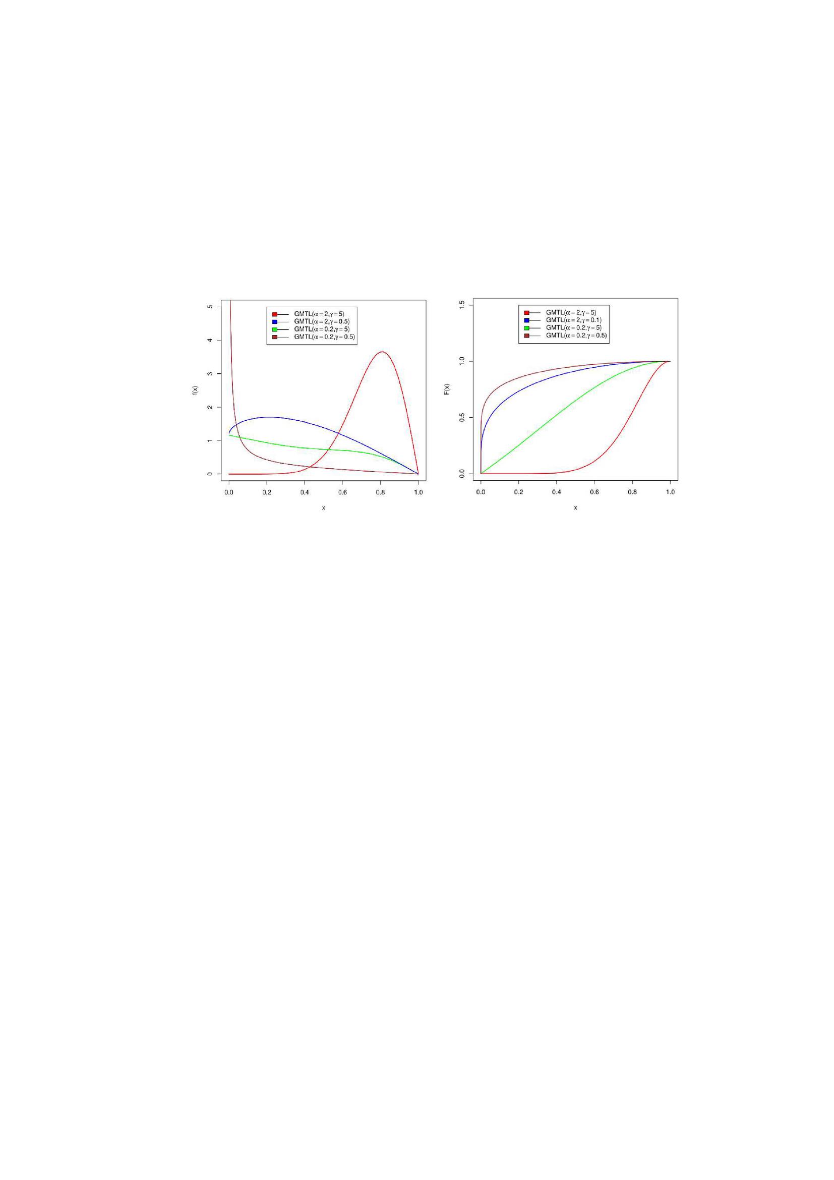
Figure 1 PDFs and CDFs of GMTL($\alpha ,\gamma$).

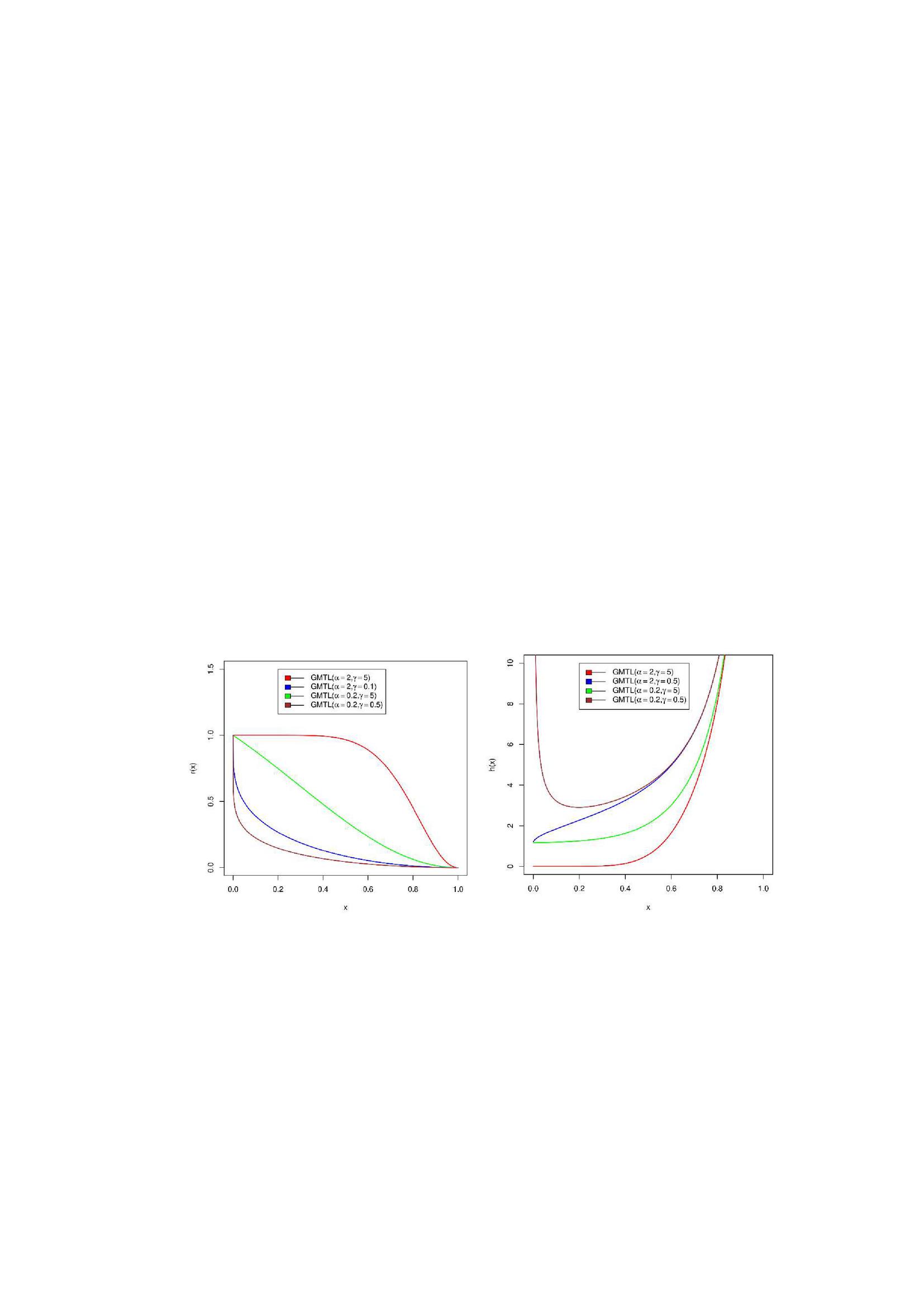
Figure 2 Reliability and hazard rate functions of GMTL($\alpha ,\gamma$).

3 Statistical Properties

3.1 Moments

The $r$th ordinary moments of the proposed distribution can be derived using the given theorem.

Theorem 3.1

$E(X^r)$	$={\displaystyle \frac{2\alpha \gamma }{e-1}}{\displaystyle \sum _{i=0}^{\mathrm{\infty }}}{\displaystyle \sum _{j=0}^{\mathrm{\infty }}}{\displaystyle \frac{1}{i!}}{(-1)}^j{2}^{\alpha \gamma +\alpha \gamma i-j-1}\left(\begin{array}{c}\hfill \alpha \gamma +\alpha \gamma \mathrm{i}-1\hfill \\ \hfill \mathrm{j}\hfill \end{array}\right)$
	$\mathrm{\hspace{1em}}\times \left({\displaystyle \frac{1}{r+\alpha \gamma +\alpha \gamma i+j}}-{\displaystyle \frac{1}{r+\alpha \gamma +\alpha \gamma i+j+1}}\right)$

Proof.

$E(X^r)$

$\mathrm{\hspace{0.5em}}={\displaystyle {\int }_0^1}{x}^{r}f(x)\mathit{d}x,$

$\mathrm{\hspace{0.5em}}={\displaystyle {\int }_0^1}{x}^r\times {\displaystyle \frac{2\alpha \gamma x^{\alpha -1}(1-x){(2-x)}^{\alpha -1}{(x^{\alpha }{(2-x)}^{\alpha })}^{(\gamma -1)}{e}^{{(x^{\alpha }{(2-x)}^{\alpha })}^{\gamma }}}{e-1}}\mathit{d}x,$

Expanding the term $e^{{(x^{\alpha }{(2-x)}^{\alpha })}^{\gamma }}={\sum }_{i=0}^{\mathrm{\infty }}{(x{(2-x)}^{\alpha \gamma })}^i/i!$ as a convergent sum of infinite terms, we get

$E(X^r)$	$={\displaystyle \frac{2\alpha \gamma }{e-1}}{\displaystyle \sum _{i=0}^{\mathrm{\infty }}}{\displaystyle \frac{1}{i!}}{\displaystyle {\int }_0^1}(1-x){(2-x)}^{\alpha \gamma +\alpha \gamma i-1}{x}^{r+\alpha \gamma +\alpha \gamma i-1}\mathit{d}x,$
	$={\displaystyle \frac{2\alpha \gamma }{e-1}}{\displaystyle \sum _{i=0}^{\mathrm{\infty }}}{\displaystyle \frac{1}{i!}}{\displaystyle {\int }_0^1}(x^{r+\alpha \gamma +\alpha \gamma i-1}-x^{r+\alpha \gamma +\alpha \gamma i}){(2-x)}^{\alpha \gamma +\alpha \gamma i-1}\mathit{d}x$

using the expansion of series,

${(2-x)}^A$	$=2^A{\left({\displaystyle \frac{2-x}{2}}\right)}^A$
	$=2^A{\left(1-{\displaystyle \frac{x}{2}}\right)}^A$
	$=2^A{\displaystyle \sum _{j=0}^{\mathrm{\infty }}}{\left({\displaystyle \frac{-1}{2}}\right)}^j\left(\begin{array}{c}\hfill \mathrm{A}\hfill \\ \hfill j\hfill \end{array}\right){(\mathrm{x})}^{\mathrm{j}}$

where, $A=\alpha \gamma +\alpha \gamma i-1$ (as per the situation) and then by further simplifying it, we get

$E(X^r)$	$={\displaystyle \frac{2\alpha \gamma }{e-1}}{\displaystyle \sum _{i=0}^{\mathrm{\infty }}}{\displaystyle \sum _{j=0}^{\mathrm{\infty }}}{\displaystyle \frac{1}{i!}}{(-1)}^j{2}^{\alpha \gamma +\alpha \gamma i-j-1}\left(\begin{array}{c}\hfill \alpha \gamma +\alpha \gamma \mathrm{i}-1\hfill \\ \hfill \mathrm{j}\hfill \end{array}\right)$
	$\mathrm{\hspace{1em}}\times \left({\displaystyle \frac{1}{r+\alpha \gamma +\alpha \gamma i+j}}-{\displaystyle \frac{1}{r+\alpha \gamma +\alpha \gamma i+j+1}}\right).$

Using Theorem 3.1, we can derive the expressions of mean, variance, skewness and kurtosis by putting the respective values of r.

3.2 Conditional Moments

The $r$th conditional moments of the proposed distribution can be derived using the given theorem.

Theorem 3.2

$E(X^r|X>t)$	$={\displaystyle \frac{2\alpha \gamma }{e-1}}{\displaystyle \sum _{i=0}^{\mathrm{\infty }}}{\displaystyle \sum _{j=0}^{\mathrm{\infty }}}{\displaystyle \frac{1}{i!}}{(-1)}^j{2}^{\alpha \gamma +\alpha \gamma i-j-1}\left(\begin{array}{c}\hfill \alpha \gamma +\alpha \gamma \mathrm{i}-1\hfill \\ \hfill \mathrm{j}\hfill \end{array}\right)$
	$\mathrm{\hspace{1em}}\times (1-t)\left({\displaystyle \frac{1}{r+\alpha \gamma +\alpha \gamma i+j}}-{\displaystyle \frac{1}{r+\alpha \gamma +\alpha \gamma i+j+1}}\right).$

Proof. To prove the above theorem, we proceed through the same way as mentioned in Theroem 3.1.

$E(X^r|X>t)$

$\mathrm{\hspace{1em}}={\displaystyle {\int }_t^1}{x}^{r}f(x)\mathit{d}x,$

$\mathrm{\hspace{1em}}={\displaystyle {\int }_t^1}{x}^r{\displaystyle \frac{2\alpha \gamma x^{\alpha -1}(1-x){(2-x)}^{\alpha -1}{(x^{\alpha }{(2-x)}^{\alpha })}^{(\gamma -1)}{e}^{{(x^{\alpha }{(2-x)}^{\alpha })}^{\gamma }}}{e-1}}\mathit{d}x,$

$\mathrm{\hspace{1em}}={\displaystyle \frac{2\alpha \gamma }{e-1}}{\displaystyle \sum _{i=0}^{\mathrm{\infty }}}{\displaystyle \frac{1}{i!}}{\displaystyle {\int }_t^1}(1-x){(2-x)}^{\alpha \gamma +\alpha \gamma i-1}{x}^{r+\alpha \gamma +\alpha \gamma i-1}\mathit{d}x,$

$\mathrm{\hspace{1em}}={\displaystyle \frac{2\alpha \gamma }{e-1}}{\displaystyle \sum _{i=0}^{\mathrm{\infty }}}{\displaystyle \frac{1}{i!}}{\displaystyle {\int }_t^1}(x^{r+\alpha \gamma +\alpha \gamma i-1}-x^{r+\alpha \gamma +\alpha \gamma i}){(2-x)}^{\alpha \gamma +\alpha \gamma i-1}\mathit{d}x$

$E(X^r|X>t)$

$\mathrm{\hspace{1em}}={\displaystyle \frac{2\alpha \gamma }{e-1}}{\displaystyle \sum _{i=0}^{\mathrm{\infty }}}{\displaystyle \sum _{j=0}^{\mathrm{\infty }}}{\displaystyle \frac{1}{i!}}{(-1)}^j{2}^{\alpha \gamma +\alpha \gamma i-j-1}\left(\begin{array}{c}\hfill \alpha \gamma +\alpha \gamma \mathrm{i}-1\hfill \\ \hfill \mathrm{j}\hfill \end{array}\right)(1-t)$

$\mathrm{\hspace{1em}\hspace{1em}}\times \left({\displaystyle \frac{1}{r+\alpha \gamma +\alpha \gamma i+j}}-{\displaystyle \frac{1}{r+\alpha \gamma +\alpha \gamma i+j+1}}\right).$

3.3 Quantile Function

To obtain the $p$th quantile function (denoted by $Q(p)$), we solve the equation $F(Q(p))=p$. Hence from Equation (3), we get

$${\{Q(p)\}}^2-2Q(p)+{\{ln(1+p(e-1))\}}^{\frac{1}{\alpha \gamma }}.$$

(9)

This equation can be further solved using the quadratic formula or by numerical methods. We have also explored the changing behavior of median with varying values of parameters $\alpha$ and $\gamma$. Thus, we put $p=0.5$ in Equation (9), where $Q(p)$ denotes the median. We get,

$${\{Q(p)\}}^2-2Q(p)+\{ln{(0.5(e+1)\}}^{1/\alpha \gamma }.$$

The nature of median with respect to changing parameters is visualized in Figure 3.

Figure 3 Variation in median with respect to changing parameters ($\alpha ,\gamma$).

3.4 Order Statistics

In this section, we obtain the probability density and cumulative distribution functions of the $r$th order statistics, which refers to the $r$th sample point in the sample of total n points, when arranged in ascending order.

Let $X_1,X_2,\mathrm{\dots },X_n$ be a random sample of size $n$, from the proposed GMTL distribution where we re-arange all the sample points in ascending order. We denote, $X_{1:n}<X_{2:n}<\mathrm{\cdots }<X_{n:n}$ as the corresponding order statistics. The pdf $f_r(x)$ of $r$th (for $r=1,2,\mathrm{\dots },n$) order statistics $X_{r:n}$ is given as,

$f_r(x)$	$={\displaystyle \frac{n!}{(r-1)!(n-r)!}}{F}^{r-1}(x){[1-F(x)]}^{n-r}f(x)$
	$={\displaystyle \frac{n!}{(r-1)!(n-r)!}}{\displaystyle \sum _{l=0}^{n-r}}{(-1)}^l\left(\begin{array}{c}\hfill n-r\hfill \\ \hfill l\hfill \end{array}\right)F^{r+l-1}(x)f(x)$

where, f(x) and F(x) denote the pdf and the cdf of the population.

And the cdf of $r$th order statistics $X_{r:n}$, $F_r(x)$, is given as

$F_r(x)$	$={\displaystyle \sum _{j=r}^n}\left(\begin{array}{c}\hfill n\hfill \\ \hfill j\hfill \end{array}\right)F^j(x){[1-F(x)]}^{n-j}$
	$={\displaystyle \sum _{j=r}^n}{\displaystyle \sum _{l=0}^{n-j}}\left(\begin{array}{c}\hfill n\hfill \\ \hfill j\hfill \end{array}\right)\left(\begin{array}{c}\hfill n-j\hfill \\ \hfill l\hfill \end{array}\right){(-1)}^l{F}^{j+l}(x).$

Thus, by using Equations (3) and (4) the pdf $f_r(x)$ and cdf $F_r(x)$ of the $r$th order statistics based on a random sample of size $n$ from the proposed distribution is derived as follows –

$f_r(x)$	$={\displaystyle \frac{n!2\alpha \gamma x^{\alpha -1}(1-x)(2-x){(x^{\alpha }{(2-x)}^{\alpha })}^{\alpha (\gamma -1)}}{(r-1)!(n-r)!}}$
	$\mathrm{\hspace{1em}}\times {\displaystyle \sum _{l=0}^{n-r}}{\displaystyle \sum _{k=0}^{\mathrm{\infty }}}{\displaystyle \frac{{(-1)}^{2r+3l-k-2}}{{(1-e)}^{r+l}}}$
	$\mathrm{\hspace{1em}}\times \left(\begin{array}{c}\hfill n-r\hfill \\ \hfill l\hfill \end{array}\right)\left(\begin{array}{c}\hfill r+l-1\hfill \\ \hfill k\hfill \end{array}\right)e^{{(x(2-x))}^{\alpha \gamma }(r+l-k-1)}$	(10)

and

$F_r(x)={\displaystyle \sum _{j=r}^n}{\displaystyle \sum _{l=0}^{n-j}}{\displaystyle \sum _{k=0}^{\mathrm{\infty }}}\left(\begin{array}{c}\hfill \mathrm{n}\hfill \\ \hfill \mathrm{j}\hfill \end{array}\right)\left(\begin{array}{c}\hfill \mathrm{n}-\mathrm{r}\hfill \\ \hfill \mathrm{l}\hfill \end{array}\right)\left(\begin{array}{c}\hfill \mathrm{j}+1\hfill \\ \hfill \mathrm{k}\hfill \end{array}\right){\displaystyle \frac{{\left(-1\right)}^{2\mathrm{j}+3\mathrm{l}-\mathrm{k}}}{{(1-e)}^{j+l}}}{e}^{{(x(2-x))}^{\alpha \gamma (j-k+l)}}.$

(11)

3.5 Mean Deviation

The mean deviation about mean is defined by,

$${\delta }_1(X)={\int }_0^1|x-\mu |f(x)\mathit{d}x,$$

where $\mu$ refers to the mean.

The above expression can be simplified as follows

$${\delta }_1(X)={\int }_0^{\mu }(\mu -x)f(x)\mathit{d}x+{\int }_{\mu }^1(x-\mu )f(x)\mathit{d}x.$$

Using integral by parts and putting $E(X)={\int }_0^{1}xf(x)\mathit{d}x=\mu$, it simplifies to

$${\delta }_1(X)=2\mu F(\mu )-2\mu +2{\int }_{\mu }^{1}xf(x)\mathit{d}x,$$

where $F(\cdot )$ denotes the proposed cdf.

By Theorem 3.2,

$${\int }_{\mu }^{1}f(x)\mathit{d}x=\frac{2\alpha \gamma }{e-1}\sum _{i=0}^{\mathrm{\infty }}\sum _{j=0}^{\mathrm{\infty }}\frac{1}{i!}{(-1)}^j{2}^{\alpha \gamma +\alpha \gamma i-j-1}$$

and thus,

${\delta }_1(X)$	$=2\mu F(\mu )-2\mu$
	$\mathrm{\hspace{1em}}+{\displaystyle \frac{2\alpha \gamma }{e-1}}{\displaystyle \sum _{i=0}^{\mathrm{\infty }}}{\displaystyle \sum _{j=0}^{\mathrm{\infty }}}{\displaystyle \frac{1}{i!}}{(-1)}^j{2}^{\alpha \gamma +\alpha \gamma i-j-1}\left(\begin{array}{c}\hfill \alpha \gamma +\alpha \gamma \mathrm{i}-1\hfill \\ \hfill \mathrm{j}\hfill \end{array}\right)(1-\mu )$
	$\mathrm{\hspace{1em}}\times \left({\displaystyle \frac{1}{r+\alpha \gamma +\alpha \gamma i+j}}-{\displaystyle \frac{1}{r+\alpha \gamma +\alpha \gamma i+j+1}}\right).$	(12)

The mean deviation about median is defined as

${\delta }_2(X)$	$={\displaystyle {\int }_0^1}|x-M|f(x)\mathit{d}x$
	$={\displaystyle {\int }_0^M}(M-x)f(x)\mathit{d}x+{\displaystyle {\int }_M^1}(x-M)f(x)\mathit{d}x,$

where $M$ refers to the median.

Ater simplying the above expression by putting $F(M)=\frac{1}{2}$, we get

$${\delta }_2(X)=-\mu +2{\int }_M^{1}xf(x)\mathit{d}x.$$

By Theorem 3.2,

${\displaystyle {\int }_M^1}xf(x)\mathit{d}x$	$={\displaystyle \frac{2\alpha \gamma }{e-1}}{\displaystyle \sum _{i=0}^{\mathrm{\infty }}}{\displaystyle \sum _{j=0}^{\mathrm{\infty }}}{\displaystyle \frac{1}{i!}}{(-1)}^j{2}^{\alpha \gamma +\alpha \gamma i-j-1}$
	$\mathrm{\hspace{1em}}\times \left(\begin{array}{c}\hfill \alpha \gamma +\alpha \gamma \mathrm{i}-1\hfill \\ \hfill \mathrm{j}\hfill \end{array}\right)(1-M)$
	$\mathrm{\hspace{1em}}\times \left({\displaystyle \frac{1}{r+\alpha \gamma +\alpha \gamma i+j}}-{\displaystyle \frac{1}{r+\alpha \gamma +\alpha \gamma i+j+1}}\right).$

Thus,

${\delta }_2(X)$	$=-\mu +{\displaystyle \frac{2\alpha \gamma }{e-1}}{\displaystyle \sum _{i=0}^{\mathrm{\infty }}}{\displaystyle \sum _{j=0}^{\mathrm{\infty }}}{\displaystyle \frac{1}{i!}}{(-1)}^j{2}^{\alpha \gamma +\alpha \gamma i-j-1}$
	$\mathrm{\hspace{1em}}\times \left(\begin{array}{c}\hfill \alpha \gamma +\alpha \gamma \mathrm{i}-1\hfill \\ \hfill \mathrm{j}\hfill \end{array}\right)(1-M)$
	$\mathrm{\hspace{1em}}\times \left({\displaystyle \frac{1}{r+\alpha \gamma +\alpha \gamma i+j}}-{\displaystyle \frac{1}{r+\alpha \gamma +\alpha \gamma i+j+1}}\right).$	(13)

3.6 Entropy

Entropy of a random variable measures the average level of information or uncertainty inherent in the variable’s possible outcomes in this section, we present the expression of Reńyi entropy (see [13]) which generalizes the Hartley and Shannon entropies. Let X has the pdf f(x) then Reńyi entropy is defined as,

$${\mathcal{𝒥}}_R(\beta )=\frac{1}{1-\beta }\log \left[\int f^{\beta }(x)\mathit{d}x\right]\mathit{\hspace{1em}}\mathrm{where}\beta >0\mathit{and}\beta \ne 1.$$

From Equation (4) we get,

${\displaystyle {\int }_0^1}{f}^{\beta }(x)\mathit{d}x={\displaystyle {\int }_0^1}{\left[{\displaystyle \frac{2\alpha \gamma }{e-1}}(1-x){(x(2-x))}^{\alpha \gamma -1}{e}^{{(x(2-x))}^{\alpha \gamma }}\right]}^{\beta }\mathit{d}x,$

and after simplification

${\displaystyle {\int }_0^1}{f}^{\beta }(x)\mathit{d}x$	$={\left[{\displaystyle \frac{2\alpha \gamma }{e-1}}\right]}^{\beta }{\displaystyle \sum _{i=0}^{\mathrm{\infty }}}{\displaystyle \sum _{j=0}^{\mathrm{\infty }}}{\displaystyle \sum _{k=0}^{\mathrm{\infty }}}{(-1)}^{j+k}{(2)}^{\alpha \beta \gamma +\alpha \beta \gamma i-\beta }$
	$\mathrm{\hspace{1em}}\times \left(\begin{array}{c}\hfill \alpha \beta \gamma +\alpha \beta \gamma \mathrm{i}-\beta \hfill \\ \hfill \mathrm{j}\hfill \end{array}\right)\left(\begin{array}{c}\hfill \beta \hfill \\ \hfill \mathrm{k}\hfill \end{array}\right)$
	$\mathrm{\hspace{1em}}\times \left({\displaystyle \frac{1}{\alpha \beta \gamma +\alpha \beta \gamma i-\beta +j+k+1}}\right).$

Hence we get

${\mathcal{𝒥}}_R(\beta )$	$={\displaystyle \frac{\beta }{1-\beta }}\log \left({\displaystyle \frac{2\alpha \gamma }{e-1}}\right)$
	$\mathrm{\hspace{1em}}+{\displaystyle \frac{1}{1-\beta }}\log \{{\displaystyle \sum _{i=0}^{\mathrm{\infty }}}{\displaystyle \sum _{j=0}^{\mathrm{\infty }}}{\displaystyle \sum _{k=0}^{\mathrm{\infty }}}{(-1)}^{j+k}{(2)}^{\alpha \beta \gamma +\alpha \beta \gamma i-\beta }$
	$\mathrm{\hspace{1em}}\times \left(\begin{array}{c}\hfill \alpha \beta \gamma +\alpha \beta \gamma \mathrm{i}-\beta \hfill \\ \hfill \mathrm{j}\hfill \end{array}\right)\left(\begin{array}{c}\hfill \beta \hfill \\ \hfill \mathrm{k}\hfill \end{array}\right)\times \left({\displaystyle \frac{1}{\alpha \beta \gamma +\alpha \beta \gamma i-\beta +j+k+1}}\right)\}.$	(14)

3.7 Stress-Strength Reliability

The stress-strength reliability is used in reliability theory as a measure of the performance of the system in consideration under stress. In terms of probability, the stress-strength reliability can be obtained as

$$R=P[X>Y],$$

where, $X$ refers to the strength of the system and $Y$ refers to the stress applied on the system.

The probability $R$ can be used to compare two random variables that come across in various disciplines.

The stress-strength reliability, $R$ for GMTL random variables where $X\sim \mathit{GMTL}({\alpha }_1,{\gamma }_1)$ and $Y\sim \mathit{GMTL}({\alpha }_2,{\gamma }_2)$ (where the parameters may or may not be equal) is given by

$R$	$={\displaystyle {\int }_0^1}\left({\displaystyle {\int }_0^x}{f}_Y(y,{\alpha }_2,{\gamma }_2)\mathit{d}y\right)f_X(x,{\alpha }_1,{\gamma }_1)\mathit{d}x$
$R$	$={\displaystyle {\int }_0^1}{f}_X(x,{\alpha }_1,{\gamma }_1)F_Y(x,{\alpha }_2,{\gamma }_2)\mathit{d}x$

on simplifying, we have,

$$R=\frac{2{\alpha }_1{\gamma }_1}{{(e-1)}^2}\left[\frac{\mathrm{\Gamma }(\frac{{\alpha }_1{\gamma }_1}{{\alpha }_1{\gamma }_1+{\alpha }_2{\gamma }_2})-\mathrm{\Gamma }(\frac{{\alpha }_1{\gamma }_1}{{\alpha }_1{\gamma }_1+{\alpha }_2{\gamma }_2},-1)}{2({\alpha }_1{\gamma }_1+{\alpha }_2{\gamma }_2){(-1)}^{\frac{{\alpha }_1{\gamma }_1}{{\alpha }_1{\gamma }_1+{\alpha }_2{\gamma }_2}}}-\frac{e-1}{2{\alpha }_1{\gamma }_1}\right]$$

(15)

where, $\mathrm{\Gamma }\cdot$ represents gamma integral and $\mathrm{\Gamma }(\cdot ,\cdot )$ represents incomplete gamma integral.

3.8 Identifiability

A family of distributions is said to be identifiable in parameters if the distribution of two members of the family are equal, i.e. $f_1(x,{\mathrm{\Theta }}_1)=f_2(x,{\mathrm{\Theta }}_2)$, then ${\mathrm{\Theta }}_1={\mathrm{\Theta }}_2$ for all values of $x$.

In order to prove our results based on identifiability, we use Theorem 1 given by [2]. It states that the density ratio, $\frac{f_1(x,{\mathrm{\Theta }}_1)}{f_2(x,{\mathrm{\Theta }}_2)}$, of two distinct (unequal parameters) members of the family defined on the interval $(a,b)$, either converges to 0 or diverges to $\mathrm{\infty }$, as $x\to a$. For the GMTL distribution, we have,

$\underset{x\to 0}{lim}{\displaystyle \frac{f_1(x,{\alpha }_1,{\gamma }_1)}{f_2(x,{\alpha }_2,{\gamma }_2)}}$	$={\displaystyle \frac{{\alpha }_1{\gamma }_1}{{\alpha }_2{\gamma }_2}}{(x(2-x))}^{{\alpha }_1{\gamma }_1-{\alpha }_2{\gamma }_2}{e}^{{(x(2-x))}^{{\alpha }_1{\gamma }_1}-{(x(2-x))}^{{\alpha }_2{\gamma }_2}}$
$\underset{x\to 0}{lim}{\displaystyle \frac{f_1(x,{\alpha }_1,{\gamma }_1)}{f_2(x,{\alpha }_2,{\gamma }_2)}}$	$=\{\begin{array}{cc}0\mathit{\hspace{1em}}\hfill & \mathrm{if}{\alpha }_1{\gamma }_1>{\alpha }_2{\gamma }_2\hfill \\ \mathrm{\infty }\mathit{\hspace{1em}}\hfill & \mathrm{if}{\alpha }_1{\gamma }_1<{\alpha }_2{\gamma }_2\hfill \\ 1\mathit{\hspace{1em}}\hfill & \mathrm{if}{\alpha }_1{\gamma }_1={\alpha }_2{\gamma }_2\hfill \end{array}$	(16)

This limit can be equal to 1 if ${\alpha }_1{\gamma }_1={\alpha }_2{\gamma }_2$. It is possible that this limit is 1 even if the parametrs are not equal to each other.

Thus, the GMTL distribution is not indentifiable as the multiplication of the two parameters may be the same for the distinct parameter values. If we parameterise the distribution using $c=\alpha \gamma$ and $\alpha =c/\gamma$, the limiting cases of the ratio of density, from Equation (16) an be given as

$$\underset{x\to 0}{lim}\frac{f_1(x,c_1,{\gamma }_1)}{f_2(x,c_2,{\gamma }_2)}=\{\begin{array}{cc}0\mathit{\hspace{1em}}\hfill & \mathrm{if}{\mathrm{c}}_1>{\mathrm{c}}_2\hfill \\ \mathrm{\infty }\mathit{\hspace{1em}}\hfill & \mathrm{if}{\mathrm{c}}_1<{\mathrm{c}}_2\hfill \\ 1\mathit{\hspace{1em}}\hfill & \mathrm{if}{\mathrm{c}}_1={\mathrm{c}}_2\hfill \end{array}$$

(17)

Thus, the GMTL parameters, $\alpha$ and $\gamma$ are identified if two members of the GMTL family have same densities with same $\gamma$ for different values of $c$ (i.e. $\alpha \gamma$).

3.9 Stochastic Ordering

A random variable $X$ is said to be stochastically greater $(X{\ge }_{st}Y)$ than $Y$ if $F_X(x)\ge F_Y(x)$ for all $x$. In a similar manner, $X$ is said to be greater than Y in the

• hazard rate order $(X{\ge }_{hr}Y)$ if $h_Y(x)\ge h_X(x)$ for all $x$

• mean residual life order $(X{\ge }_{mlr}Y)$ if $m_X(x)\ge m_Y(x)$ for all $x$

• likelihood ratio order $(X{\ge }_{lr}Y)$ if $\frac{f_X(x)}{f_Y(x)}$ is an increasing function of $x$

Theorem 3.3 Letus have two independent random variables X and Y, such that $X\sim \mathit{GMTL}({\alpha }_1,{\gamma }_1)$ and $Y\sim \mathit{GMTL}({\alpha }_2,{\gamma }_2)$. Then, we have the following conditions

1. For ${\gamma }_1={\gamma }_2=\gamma$ and ${\alpha }_1\ge {\alpha }_2$, $(X{\ge }_{lr}Y)$, $(X{\ge }_{mlr}Y)$, $(X{\ge }_{hr}Y)$ and $(X{\ge }_{st}Y)$ for all $x$.

2. For ${\alpha }_1={\alpha }_2=\alpha$ and ${\gamma }_1\ge {\gamma }_2$, $(X{\ge }_{lr}Y)$, $(X{\ge }_{mlr}Y)$, $(X{\ge }_{hr}Y)$ and $(X{\ge }_{st}Y)$ for all $x$.

Proof. The likelihood ratio of two independent random variables $X$ and $Y$ is given by

$$\frac{f_X(x;{\alpha }_1,{\gamma }_1)}{f_Y(x;{\alpha }_2,{\gamma }_2)}=\frac{{\alpha }_1{\gamma }_1}{{\alpha }_2{\gamma }_2}{(x(2-x))}^{{\alpha }_1{\gamma }_1-{\alpha }_2{\gamma }_2}{e}^{{(x(2-x))}^{{\alpha }_1{\gamma }_1}-{(x(2-x))}^{{\alpha }_2{\gamma }_2}}$$

We first consider Case I, ${\gamma }_1={\gamma }_2=\gamma$ and differentiate the above likelihood ratio with respect to $x$. It gives

$$\frac{d}{dx}\left(\frac{f_X(x;{\alpha }_1,\gamma )}{f_Y(x;{\alpha }_2,\gamma )}\right)=\frac{2{\alpha }_1\gamma }{{\alpha }_2}\frac{({\alpha }_1-{\alpha }_2)(1-x){(x(2-x))}^{({\alpha }_1-{\alpha }_2)\gamma }}{x(2-x)}.$$

(18)

For ${\alpha }_1>{\alpha }_2$, $\frac{d}{dx}(\frac{f_X(x;{\alpha }_1,\gamma )}{f_Y(x;{\alpha }_2,\gamma )})>0,$ for all $x$. Thus, the likelihood ratio increases as the value of x increases (increasing function of x). Hence, for ${\gamma }_1={\gamma }_2=\gamma$, $(X{\ge }_{lr}Y)$. Now, by the result provided by [16], $(X{\ge }_{lr}Y)\Rightarrow (X{\ge }_{hr}Y)(X{\ge }_{mlr}Y)$ and $(X{\ge }_{st}Y)$. Similarly, we consider the Case II, ${\alpha }_1={\alpha }_2=\alpha$, and proceed in a similar way as above

$$\frac{d}{dx}\left(\frac{f_X(x;\alpha ,{\gamma }_1)}{f_Y(x;\alpha ,{\gamma }_2)}\right)=\frac{2{\gamma }_1\alpha }{{\gamma }_2}\frac{({\gamma }_1-{\gamma }_2)(1-x){(x(2-x))}^{({\gamma }_1-{\gamma }_2)\alpha }}{x(2-x)}.$$

(19)

For ${\gamma }_1>{\gamma }_2$, $\frac{d}{dx}(\frac{f_X(x;\alpha ,{\gamma }_1)}{f_Y(x;\alpha ,{\gamma }_2)})>0,$ for all $x$. Thus, the likelihood ratio increases as the value of x increases (increasing function of x). Hence, for ${\alpha }_1={\alpha }_2=\alpha$, $(X{\ge }_{lr}Y)$. Now, by the result provided by [16], $(X{\ge }_{lr}Y)\Rightarrow (X{\ge }_{hr}Y)(X{\ge }_{mlr}Y)$ and $(X{\ge }_{st}Y)$.

3.10 Ordinary Differential Equations for Density and Survival Functions

We obtain the first order differential equations of density and survival functions of the proposed GMTL distribution. It is done by calculating the first derivatives of density and survival functions with respect to x.

The first order derivative of the pdf is

$f^{\prime }(x)$	$=\left({\displaystyle \frac{2\alpha \gamma }{e-1}}\right){(x(2-x))}^{\alpha \gamma -1}(1-x)e^{{(x(2-x))}^{\alpha \gamma }}$
	$\mathrm{\hspace{1em}}\times \left[{\displaystyle \frac{2\alpha \gamma {(x(2-x))}^{\alpha \gamma }{(1-x)}^2+(2\alpha \gamma -1){(1-x)}^2-1}{x(2-x)(1-x)}}\right].$

Thus, the first order ODE for density function, by re-arranging the above expression into a more meaningful form, is

$$y^{\prime }-\left[\frac{2\alpha \gamma {(x(2-x))}^{\alpha \gamma }{(1-x)}^2+(2\alpha \gamma -1){(1-x)}^2-1}{x(2-x)(1-x)}\right]y=0.$$

(20)

Table 1 Ordinary differential equations of GMTL density

First Order
$\alpha$	$\gamma$	First Order ODE
1	1	$y^{\prime }-\left\{{\displaystyle \frac{2(x(2-x)){(1-x)}^2+{(1-x)}^2-1}{x(2-x)(1-x)}}\right\}y=0$
2	1	$y^{\prime }-\left\{{\displaystyle \frac{4{(x(2-x))}^2{(1-x)}^2+3{(1-x)}^2-1}{x(2-x)(1-x)}}\right\}y=0$
3	1	$y^{\prime }-\left\{{\displaystyle \frac{6{(x(2-x))}^3{(1-x)}^2+5{(1-x)}^2-1}{x(2-x)(1-x)}}\right\}y=0$

Table 2 Ordinary differential equations of GMTL survival function

First Order
$\alpha$	$\gamma$	First Order ODE
1	1	$z^{\prime }+2(1-x)\log [(1-z)(e-1)+1][(1-z)(e-1)+1]=0$
2	1	$z^{\prime }+4(1-x)\log [(1-z)(e-1)+1][(1-z)(e-1)+1]=0$
3	1	$z^{\prime }+6(1-x)\log [(1-z)(e-1)+1][(1-z)(e-1)+1]=0$

where, $y=f(x)$ and $y^{\prime }=\frac{df(x)}{dx}$. We present the first order ODEs of the pdf, for some considered parameters, in Table 1.

The survival function of the GMTL distribution given by $z=S_X(x)=1-\frac{e^{{(x(2-x))}^{\alpha \gamma }}-1}{e-1}$.

On differentiating it w.r.t. x, we have

$$z^{\prime }=-2\alpha \gamma (1-x){(x(2-x))}^{\alpha \gamma }{e}^{{(x(2-x))}^{\alpha \gamma }}$$

Thus, on simplifying the above expression and re-arranging it we have,

$$z^{\prime }+2\alpha \gamma (1-x)\log [(1-z)(e-1)+1][(1-z)(e-1)+1]=0$$

(21)

where, $z=S_X(x)$ and $z^{\prime }=\frac{d{S}_X(x)}{dx}$. For some considered values of the parameters, first order ODEs of the survival function are presented in Table 2.

4 Maximum Likelihood Estimation and Simulation

4.1 Point Estimation

We obtain the maximum likelihood estimators of the parameters $\alpha$ and $\gamma$ by maximising the likelihood or log-likelihood function with respect to x. The log-likelihood function from the proposed distribution usig a sample of size n is given by,

$\log L$	$=n\log {\displaystyle \frac{2}{e-1}}+n\log (\alpha )+nlog(\gamma )+{\displaystyle \sum _{i=1}^n}log(1-x_i)+(\alpha \gamma -1)$
	$\mathrm{\hspace{1em}}\times {\displaystyle \sum _{i=1}^n}log(x_i(2-x_i))+{\displaystyle \sum _{i=1}^n}{(x_i(2-x_i))}^{\alpha \gamma }$	(22)

Differentiating it with respect to the both parameters separately we get,

${\displaystyle \frac{d\log L}{d\alpha }}$	$={\displaystyle \frac{n}{\alpha }}+\gamma {\displaystyle \sum _{i=1}^n}log(x_i(2-x_i))$
	$\mathrm{\hspace{1em}}+\gamma {\displaystyle \sum _{i=1}^n}{(x_i(2-x_i))}^{\gamma \alpha }log(x_i(2-x_i))$

and

${\displaystyle \frac{d\log L}{d\gamma }}$	$={\displaystyle \frac{n}{\gamma }}+\alpha {\displaystyle \sum _{i=1}^n}log(x_i(2-x_i))$
	$\mathrm{\hspace{1em}}+\alpha {\displaystyle \sum _{i=1}^n}{(x_i(2-x_i))}^{\gamma \alpha }log(x_i(2-x_i)).$

In order to get the point estimates, we equate both the equations to zero. We get the MLEs $\widehat{\alpha }$ and $\widehat{\gamma }$ of parameters $\alpha$ and $\gamma$ respectively.

We obtain the MLEs $\widehat{\alpha }$ and $\widehat{\gamma }$ of the parameters $\alpha$ and $\gamma$ respectively by equating the above equations to zero and solving the two non-linear equations. These equations may not be solved by any analytical methods. Thus, use of numerical methods is required. We recommend the use of Newton Raphson method where the initial choice of roots might be obtained using the contour plots.

4.2 Asymptotic Confidence Intervals

In this section, we obtain the confidence intervals of the parameters on the basis of the asymptotic properties of the maximum likelihood estimators. We use the diagonal elements of the Fisher information matrix $I^{-1}(\widehat{\alpha },\widehat{\gamma })$ and use the estimators of its elements to obtain the estimated asymptotic variance for the parameters $\alpha$ and $\gamma$ respectively. As this is an asymptotic propery, it is only valid for large sample problems.

Thus, two sided $100(1-\beta )\%$ confidence interval of $\alpha$ and $\gamma$ can be defined as $\widehat{\alpha }\pm Z_{\beta /2}\sqrt{var(\widehat{\alpha })}$ and $\widehat{\gamma }\pm Z_{\beta /2}\sqrt{var(\widehat{\gamma })}$ respectively. Where $Z_{\beta /2}$ denotes the upper $\beta /2\%$ point of standard normal distribution. Fisher Information matrix can be estimated by,

$$I(\widehat{\alpha },\widehat{\gamma })={\left[\begin{array}{cc}\frac{-d^2\log L}{d{\alpha }^2}\mathit{\hspace{1em}}\hfill & \frac{-d^2\log L}{d\alpha d\gamma }\hfill \\ \frac{-d^2\log L}{d\alpha d\gamma }\mathit{\hspace{1em}}\hfill & \frac{-d^2\log L}{d{\gamma }^2}\hfill \end{array}\right]}_{(\widehat{\alpha },\widehat{\gamma })}$$

(23)

where,

${\displaystyle \frac{d^2\log L}{d{\alpha }^2}}$	$={\displaystyle \frac{-n}{{\alpha }^2}}+{\gamma }^2{\displaystyle \sum _{i=1}^n}{(x_i(2-x_i))}^{\gamma \alpha }{[\log x_i(2-x_i)]}^2$
${\displaystyle \frac{d^2\log L}{d{\gamma }^2}}$	$={\displaystyle \frac{-n}{{\gamma }^2}}+{\alpha }^2{\displaystyle \sum _{i=1}^n}{(x_i(2-x_i))}^{\gamma \alpha }{[\log x_i(2-x_i)]}^2$
${\displaystyle \frac{d^2\log L}{d\alpha d\gamma }}$	$={\displaystyle \sum _{i=1}^n}\log (x_i(2-x_i))$
	$\mathrm{\hspace{1em}}+{\displaystyle \sum _{i=1}^n}{(x_i(2-x_i))}^{\alpha \gamma }\log (x_i(2-x_i))[\log (x_i(2-x_i))\alpha \gamma +1]$

4.3 Random Number Generation

The steps to generate random numbers from the proposed $\mathit{GMTL}(\alpha ,\gamma )$ distribution are –

1. Select $n,\alpha$ and $\gamma$.

2. Generate a standard uniform random number, $u\sim U(0,1)$.

3. Using the quantile function, compute

$$x=1-\sqrt{1-{\{\log (1+u(e-1))\}}^{1/\alpha \gamma }}.$$

4. Repeat the steps 2 and 3, $n$ times to get a sample of size $n$, $\{x_1,x_2,\mathrm{\dots },x_n\}$ from $\mathit{GMTL}(\alpha ,\gamma )$.

Illustration:

1. We fix $n=10,\alpha =2$ and $\gamma =3.$

The random sample generated is: {0.7575, 0.7344, 0.9391, 0.7976, 0.6713, 0.8507, 0.4252, 0.7743, 0.7354, 0.7549}

2. We fix $n=20,\alpha =5$ and $\gamma =1.$

The random sample generated is: {0.5901, 0.6160, 0.8302, 0.7302, 0.7026, 0.3785, 0.4896, 0.6976, 0.4615, 0.7156, 0.5139, 0.8669, 0.8872, 0.7725, 0.5092, 0.7548294 0.5602, 0.5448, 0.8950, 0.3764}

4.4 Simulation Study

In order to prove the consistency of the maximum likelihood estimators, of the parameters, we conduct an extensive simulation study. In this study, we simulate 10000 samples for the given value of parameters for increasing values of n (i.e., n $=$ 20,40,…200). We then compute MSE and mean absolute bias of the MLEs on the basis of these samples and study the performance of mean squared error and mean absolute bias as a function of sample size. The MSE and mean absolute bias (AB) are computed using the following formulae,

$\mathit{MSE}(\widehat{\alpha })$	$={\displaystyle \frac{1}{10000}}{\displaystyle \sum _{j=1}^{10000}}{({\widehat{\alpha }}_j-\alpha )}^2,AB(\widehat{\alpha })={\displaystyle \frac{1}{10000}}{\displaystyle \sum _{j=1}^{10000}}|{\widehat{\alpha }}_j-\alpha |,$
$\mathit{MSE}(\widehat{\gamma })$	$={\displaystyle \frac{1}{10000}}{\displaystyle \sum _{j=1}^{10000}}{({\widehat{\gamma }}_j-\gamma )}^2,AB(\widehat{\gamma })={\displaystyle \frac{1}{10000}}{\displaystyle \sum _{j=1}^{10000}}|{\widehat{\gamma }}_j-\gamma |.$

We present the results of simulation study for parameters, ($\alpha ,\gamma$)= (0.5,1.5) in Table 3 and the results are visualized in Figure 4.

Table 3 Mean squared error and mean absolute bias for ($\alpha ,\gamma$) for simulated samples

$(\alpha ,\gamma )=(0.5,1.5)$
Sample Size	MSE($\widehat{\alpha }$)	AB($\widehat{\alpha }$)	MSE($\widehat{\gamma }$)	AB($\widehat{\gamma }$)
20	0.0165	0.0966	0.0013	0.0292
40	0.0071	0.0653	0.0006	0.0203
60	0.0045	0.0525	0.0004	0.0169
80	0.0034	0.0461	0.0003	0.0157
100	0.0026	0.0404	0.0002	0.0135
120	0.0021	0.0369	0.0002	0.0122
140	0.0019	0.0345	0.0002	0.0114
160	0.0016	0.0319	0.0001	0.0105
180	0.0014	0.0302	0.0001	0.0100
200	0.0012	0.0284	0.0001	0.0094

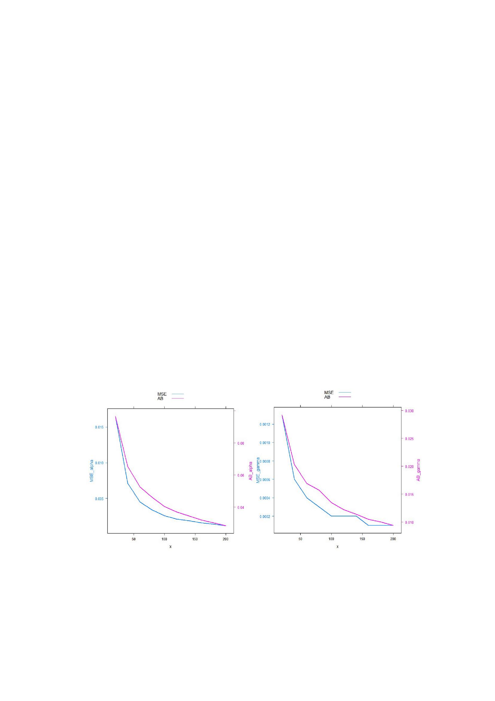
Figure 4 MSE and mean absolute bias of $\widehat{\alpha }$ and $\widehat{\gamma }$ for simulated samples with $\alpha =0.5$ and $\gamma =1.5$.

From Figure 4, it can be concluded that the mean squared error and mean absolute bias decrease as the sample size (n) increases for 10000 simulated samples. This proves that the maximum likelihood estimators are consistent.

5 Real Data Fitting

In this section, we analyze a real dataset in order to illustrate the performance of the proposed GMTL($\alpha ,\gamma$) distribution. The GMTL distribution is fitted to the data of recovery rates of CD34$+$ cells after peripheral blood stem cell (PBSC) transplants. The study was conducted with 239 patients between 2003 and 2008 at the Edmonton Hematopoietic Stem Cell Lab in Cross Cancer Institute-Alberta Health Services. The data is present in R package {simplexreg} (refer R Core Team (2013) [14]), by the title sdac. The recovery rates can be extracted using the command sdac$rcd. We have used $\alpha =5$ and $\gamma =2$ as initial values of the iterative algorithm. Thus, the obtained MLEs of the parameters of the GMTL distribution are: $\widehat{\alpha }=5.1644$ and $\widehat{\gamma }=2.4269$.

Figure 5 gives the fitting of different models that are considered over the given data set (refer Sharma(2020) [18]). The K-S statistic for the fitting is 0.0544, with p-value 0.8713. It suggests that the proposed GMTL distribution is quite suitable for fitting of this data.

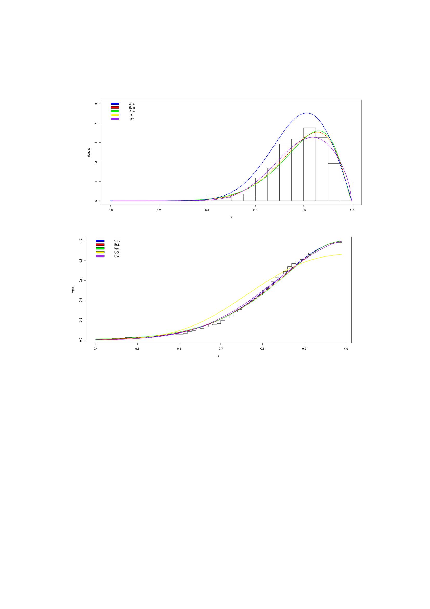
Figure 5 Fitting of different models on the given dataset.

Further, we compare the goodness-of-fit statistics with Beta, Kumaraswamy, unit-Gamma and unit-Weibull distributions which are also defined on the unit interval. We use some criteria like- Akaike Information Criterion (AIC) and Bayesian Information Criterion (BIC) to compare the models under consideration and identify the best possible model for the given data set. The model with the smallest values of AIC and BIC statistics is considered to be the best possible model among the distributions under comparison. The statistics are computed by

$\mathit{AIC}$	$=2k-2\mathrm{l}\mathrm{o}\mathrm{g}(L)$
$\mathit{BIC}$	$=k\log (n)-2\mathrm{l}\mathrm{o}\mathrm{g}(L)$

where, $k$ is the number of estimated parameters, $L$ is the maximum value of likelihood function and $n$ is the number of observations. We also use the K-S statistics and their corresponding p-values for comparison of different models. The model having the smallest value of the K-S statistic is considered to be the best model amongst all the models under consideration.

Table 4 presents the MLEs, maximum values of log-likelihood functions, AIC and BIC criteria along with the K-S statistics and the p-values. From the table, we conclude that the proposed GDUS-Modified Topp Leone (GMTL) distribution has the highest log (L) value, smallest values of AIC, BIC and K-S- statistics among the all distributions under consideration. Therefore, we recommend the use of the proposed GMTL distribution for modelling the given dataset over the existing datat sets over the unit range which were considered.

Table 4 Maximum value of log(L), MLEs, AIC, BIC, K-S statistics and p-values for various fitted models

Comparison of Distributions
Model	$log(L)$	MLEs	AIC	BIC	K-S statistic	p-value
GMTL($\alpha ,\gamma$)	192.8600	(5.1644,2.4269)	-381.7200	-374.7671	0.0544	0.8713
Beta($\alpha ,\beta$)	191.8672	(8.6671,2.2859)	-379.7345	-372.7816	0.0669	0.6578
Kumaraswamy ($\alpha ,\beta$)	190.7640	(6.6942,2.4535)	-379.5280	-370.5751	0.0753	0.5067
Unit-Gamma($\alpha ,\beta$)	191.8867	(2.2808,9.2516)	-379.7734	-372.8205	0.1380	0.0210
Unit-Weibull($\alpha ,\beta$)	192.0157	(8.0559,1.6181)	-380.0314	-373.0785	0.0585	0.8068

6 Conclusion

In this paper, a two-parameter extension of the J-shaped Topp-Leone distribution called as GDUS-Modified Topp-Leone (GMTL) distribution is introduced for a possible application of modeling of recovery rates of CD34+ cells after peripheral blood stem cell (PBSC) transplants. The proposed distribution has an interesting property to accommodate variety of density and hazard rate functions like increasing, decreasing, and bathtub shapes. The expressions of ordinary moments, conditional moments, quantile function, mean deviation, order statistics, and entropy are discussed. Other important properties of the proposed distribution like- identifiability, ordinary differential equations, stochastic orderings, and stress-strength reliability are also discussed (also refer [19]).

The estimation techniques for the parameters are also discussed. The simulation study that was conducted proved the consistency of the ML estimators of the parameters. Further, an algorithm for the generation of a random sample from the proposed distribution is also given to facilitate future studies.

According to the various goodness-of-fit criteria, like AIC, BIC, and K-S statistics, the proposed GMTL distribution is a better model for fitting the recovery rates of CD34$+$ cells data over the Beta, Kumaraswamy, unit-Gamma, and unit-Weibull distributions (also refer [18]). Summing up, it can be concluded that the GMTL distribution can be effectively used for modeling real data defined on the unit interval.

References

[1] M. Alizadeh, F. Lak, M. Rasekhi, T. G. Ramires, H. M. Yousof, and E. Altun. The odd log-logistic topp-leone g family of distributions: heteroscedastic regression models and applications. Comput. Stat., 33, 3:1217–1244, 2018.

[2] A. P. Basu and J. K. Ghosh. Identifiability of distributions under competing risks and complementary risks model. Communications in Statistics – Theory and Methods, 9:1515–1525, 1980.

[3] P.C. Consul and G.C. Jain. On the log-gamma distribution and its properties. Stat Pap, 12:100–106, 1971.

[4] E. Gómez-Déniz, M.A. Sordo, and E. Calderín-Ojeda. The log-lindley distribution as an alternative to the beta regression model with applications in insurance. Insur Math Econ, 54:49–57, 2014.

[5] N.L. Johnson. Systems of frequency curves generated by methods of translation. Biometrika, 36(1/2):149–176, 1949.

[6] P. Kumaraswamy. A generalized probability density function for double-bounded random processes. J Hydrol, 46(1-2):79-88, 1980.

[7] M.Ç. Korkmaz and C. Chesneau. On the unit burr-xii distribution with the quantile regression modeling and applications. Comp. Appl. Math., 40(1), 2021.

[8] S.K. Maurya, A. Kaushik, S.K. Singh, and U. Singh. A new class of distribution having decreasing, increasing, and bathtub-shaped failure rate. Commun. Stat. Theory Methods, 46, 20:10359–10372, 2017.

[9] J. Mazucheli and S. Dey A.F. Menezes. The unit-birnbaum-saunders distribution with applications. Chile J Stat, 9(1):47–57, 2018.

[10] J. Mazucheli, A.F.B. Menezes, and M.E. Ghitany. The unit-weibull distribution and associated inference. J Appl Probab Stat, 13:1–22, 2018.

[11] J. Mazucheli, A.F. Menezes, and S. Dey. Unit-gompertz distribution with applications. Statistica, 79(1):25–43, 2019.

[12] S. Nadarajah and S. Kotz. Moments of some j-shaped distributions. J. Appl. Stat., 35, 10:1115–1129, 2003.

[13] A. Renyi. On measures of entropy and information. In Proceedings of the 4th Berkeley symposium on mathematical statistics and probability. Berkeley :University of California Press., 1:547–561, 1961.

[14] R Core Team. R: A Language and Environment for Statistical Computing. R Foundation for Statistical Computing, Vienna, Austria, 2013.

[15] Y. Sangsanit and W. Bodhisuwan. The topp-leone generator of distributions: properties and inferences. Songklanakarin. J. Sci. Technol., 38:537–548, 2016.

[16] M. Shaked and J. Shanthikumar. Stochastic orders and their applications. Academic Press, Boston, 1994.

[17] V.K. Sharma. Topp-leone normal distribution with application to increasing failure rate data. Journal of Statistical Computation and Simulation, 83, 2:326–339, 2018.

[18] V.K. Sharma. R for lifetime data modeling via probability distributions. Handbook of Probabilistic Models, Elsevier Inc., 2020.

[19] K. Shekhawat and V.K. Sharma. An extension of J-shaped distribution with application to tissue damage proportions in blood. Sankhya B, 83:543–574, 2021.

[20] C. W. Topp and F. C. Leone. A family of J-shaped frequency functions. J. Am. Stat. Assoc., 50:209–219, 1955.

[21] M. N. Shahzad, Z. Asghar, Transmuted Power Function Distribution: A More Flexible Distribution, Journal of Statistics and Management Systems 19(4) (2016) 519–539.

[22] Tanış, C. (2021) On Transmuted Power Function Distribution: Characterization, Risk Measures, and Estimation. Journal of New Theory, (34), 72–81.

[23] Karakaya, K., Kınacı, İ., Kuş, C., Akdoğan, Y. (2021). On the DUS-Kumaraswamy Distribution. Istatistik Journal of The Turkish Statistical Association, 13(1), 29–38.

[24] Kumar, D., Singh, U. and Singh, S.K. (2015). A Method of Proposing New Distribution and its Application to Bladder Cancer Patients Data. J. Stat. Appl. Pro. Lett., 2(2), 235–245.

Biographies

Arun Kaushik is currently working as an Assistant Professor in the Department of Statistics, Banaras Hindu University, Varanasi, India. He completed his PhD in Statistics in 2016. His research interests span the areas of Bayesian Inference, decision theory, MCMC, distribution theory, Bayesian econometrics, Python language, and STAN Software applications. He has been a recipient of CSIR JRF and CSIR SRF during PhD.

Unnati Nigam is currently a Masters’ degree student in the Department of Statistics, Banaras Hindu University, Varanasi, India. She completed her graduation from the same university in the year 2020 with a Gold Medal. She aspires to research and contribute in the areas of Statistical Inference, Bayesian Inference, Lifetime Data Analysis, Distribution Theory and R-software applications.

Journal of Reliability and Statistical Studies, Vol. 15, Issue 1 (2022), 299–324.
doi: 10.13052/jrss0974-8024.15112
© 2022 River Publishers