A Copula Based Stress-Strength Reliability Estimation with Lindley Marginals

A. James¹, N. Chandra^1,* and M. Pandey²

¹Department of Statistics, Ramanujan School of Mathematical Sciences, Pondicherry University, Puducherry – 605 014, India
²Department of Zoology and DST Centre for Mathematical Sciences, Institute of Sciences, Banaras Hindu University, Varanasi 221 005, India
E-mail: nc.stat@gmail.com
*Corresponding Author

Received 15 October 2021; Accepted 26 April 2022; Publication 28 May 2022

Abstract

The stress-strength model is a basic tool used in evaluating the reliability (R). It shows that a component or system with stress (Y) and strength (X) will fail if the stress exceeds the strength, and its counterpart allows it to function. Usually, the statistical independence between X and Y are assumed and reliability models are extensively developed in the literature. However, in real life, there are many situations in which the dependence stress-strength is taken into account. So it is important to consider and model the association between them. In this paper, we estimated R when the stress and strength parameters are linked by a Fralie-Gumble-Morgenstern copula with Lindley marginals. The estimates of reliability and dependence parameter are obtained by using maximum likelihood estimation (MLE), inference function margins (IFM), and semi parametric (SP) methods. In addition, the length of the asymptotic confidence interval and the coverage probability of the dependence parameter are also computed. A simulation study is performed to evaluate the effectiveness of the various estimates, and a real data set is also used for illustrative purposes.

Keywords: Stress-strength reliability, Lindley distribution, Fralie-Gumble-Morgenstern, maximum likelihood estimation, inference function margins, semi-parametric method, Monte-Carlo simulation.

1 Introduction

Lindley (1958, 1965) [34, 33] firstly proposed Lindley distribution in the context of fiducial Bayesian statistics. In the recent years, Lindley distribution has attracted the researchers due to its dominating characteristics over exponential and weibull distributions. It has been widely used in several disciplines like, medical, engineering, finance, etc., where modeling and analyzing lifetime data are vital. Ghitany et al. (2008) [21] studied several statistical properties and maximum likelihood estimation of the parameters of Lindley distribution. Further, they reported that Lindley distribution is a special mixture of exponential($\theta$) and gamma(2,$\theta$) and observed that Lindley distribution is the best fit as compared to exponential distribution for bank service time data. Mazucheli and Achcar (2011) [35] analyzed competing risk lifetime data using the Lindley distribution. Gupta and Singh (2013) [22] investigated the hybrid censored lifetime data by using classical and Bayesian techniques on the assumption that lifetime follows the Lindley distribution.

Many researchers worked on modifications of Lindley distribution by combining it with other life distributions to make it more flexible to model time to failure data. For instance, weighted Lindley distribution by Ghitany et al. (2011) [20], extended Lindley distribution proposed by Bakouch et al. (2012) [5], the exponential Poisson Lindley distribution by Barreto- Souza and Bakouch (2013) [8] and quasi Lindley distribution introduced by Shanker and Mishra (2013) [47]. Recently, a new unit-improved second-degree Lindley distribution was introduced by Altun and Cordeiro (2020 [3], XLindley distribution by Sarra and Zeghdoudi (2021) [44] and Odd Lindley Burr XII Model proposed by Korkmaz and Hamedani (2018) [38].

In this article, we use the two-parameter Lindley distribution introduced by Shanker et al. (2013) [48], to estimate the stress-strength reliability using copula function. The motivation behind to assume Lindley distribution is that because it is quite suitable to model real data than the other well known life distributions. The probability density function (p.d.f) and cumulative distribution function (c.d.f) of two-parameter Lindley distribution are given by

$f_X(x;\alpha ,\theta )$	$={\displaystyle \frac{{\theta }^2}{\theta +\alpha }}(1+\alpha x)e^{-\theta x},x>0,\theta >0,\alpha >-\theta ,$	(1)
$F_X(x;\alpha ,\theta )$	$=1-{\displaystyle \frac{\theta +\alpha +\alpha \theta x}{\theta +\alpha }}{e}^{-\theta x},x>0,\theta >0,\alpha >-\theta .$	(2)

When $\alpha =1$, then the distribution in (1) and (2) reduces to the corresponding p.d.f and c.d.f of one parameter Lindley distribution and $\alpha =0$ it reduces to exponential distribution.

The above p.d.f can be expressed as

$$f_X(x;\alpha ,\theta )=p{f}_1(x)+(1-p)f_2(x),$$

(3)

where $f_1(x)=\theta e^{-\theta x}$ and $f_2(x)={\theta }^{2}x{e}^{-\theta x}$. Thus two parameter Lindley distribution is a mixture of exponential $(\theta )$ and gamma $(2,\theta )$ with mixing proportions $p=\frac{\theta }{\theta +\alpha }$ and $(1-p)=\frac{\alpha }{\theta +\alpha }$ respectively.

In reliability analysis, stress-strength models usually describes to access the impact of two quantities on a electrical or electronic system. The system reliability under stress-strength setup is defined by $R=P(Y<X)$, which measures the system’s probability of performing its intended function. The idea of stress-strength reliability has been widely applied in several disciplines. For example, in engineering sciences, stress-strength reliability models are used to estimate the system reliability R. In medical sciences, R can be used to estimate the amount (effect) of drug administered between two population groups. In addition to this, it is also used extensively in economics, sociology, psychology, behavioural sciences, agricultural sciences, aeronautical and military sciences. Basically, the problem of stress-strength reliability estimation was initiated around seven decades ago see, Birnbaum and McCarty (1958) [10] and later, the idea of stress-strength has been gradually spread over all the important disciplines of science and humanities till the twenty first century, since it has potential to measure of distinguish between more than two population distributions.

In literature, a reasonable amount of work in this direction has been attempted by several authors by considering both stress and strength follow some well-known either same or different families of univariate life distributions, whereas stress (Y) and the strength (X) are assumed independent and identically distributed (i.i.d) as well as independent and non-identically distributed random variables. Al-Mutairi et al. (2013) [2] attempted the estimation of stress-strength reliability for Lindley variables with different shape parameters by adopting UMVUE, MLE, and Bayes approach. Asymptotic confidence interval, bootstrap confidence intervals, and Credible interval of R has been proposed. Singh et al. (2014) [50] have proposed estimation of system reliability for generalized Lindley stress-strength model. Ghitany et al. (2015) [19] discuss the point and interval estimation of R for power Lindley distribution based on MLE, nonparametric and bootstrap methods. Sharma et al. (2015) [49] described stress-strength reliability model for inverse Lindley distribution with applications to head and neck cancer data. Khan and Jan (2015) [27] considered the MLE of R by assuming strength follows a finite mixture of two-parameter Lindley and stress follows exponential distributions. Biswas et al. (2021) [11] drawn inferences on R with log-Lindley distribution under both classical and Bayesian set-up, and an application to insurance and financial credibility is discussed. A complete review on stress-strength reliability modelling is given in Kotz and Pensky (2003) [29]. Some of very recent contributions in this direction are, Kundu and Raqab (2015) [31], Rostamian and Nematollahi (2019) [42], Chandra and Rathaur (2020) [13], Baro-Tijerina et al. (2020) [7] and references therein. In aforesaid attempts, the prime reason for choosing independence between these two variables is its mathematical and computational simplicity.

Later, some amount of work on estimation of stress-strength reliability of multi-component system is available in the literature by assuming either dependent stresses with common strength or otherwise for bivariate types of life distributions (e.g., exponential, normal, log-normal, Pareto and gamma margins) see, Gupta and Subramanian (1998) [23], Chandra and Pandey (2012) [12] and references therein. These attempts have focused only on estimating reliability rather than exploring the different forms of the dependence relationship between the stresses or strengths or otherwise and estimating the dependence parameter.

However, in real life, there are situations in which the dependence between stress-strength is taken into account. Some real life scenarios are:

1. In engineering application, an electric or electronic supersonic system is configured (desired strength) with the desired number of subsystems or components. Assume each of these components is associated and functioning. If one of the components is disconnected or weaker, then the system lacks full performance. Hence it is important to measure the level of dependence among the components in terms of stress and strength variables.

2. In medical application, a pharmaceutical manufacturing company produces new drugs, a proportion of several substances are mixed for a desired capacity of a drug (in mg) to resist(strength) the effect on diseases to kill off the harmful viruses(stress) in the individual body, where each of substances used in a drug are chemically associated in performing their combined effect.

3. In social and political system, a political ruling party may run the stable government and have inherent bureaucratic and constitutional power (strength) for better survival for a desired period but government may fail to survive if they fail to address the challenges in different sectors of humanities. Where failure of internal social security issues, dispute of neighbor states/countries, strikes, war, terrorist attacks, cyber-attacks etc. are various kinds of sensitive issues may becomes stresses for ruling party.

So it is therefore important to consider and model the association between stress (Y) and the strength (X). One way to model the dependence between X and Y is using copulas when marginal distributions are known. But until now, only very few works cited in the literature on the estimation of stress-strength reliability in a dependence setup. Domma and Giordano (2013) [16] considered Farlie–Gumbel–Morgenstern (FGM) and generalized FGM copula to estimate R with Burr system of margins. Vaidyanathan and Sharon (2016) [53] derived the expression of stress-strength reliability when X and Y follow one parameter Lindley distribution. Ahmed et al. (2020) [1] studied the estimation of R based on MLE, IFM and Bayesion estimation approach. A very recent development on independent and dependent stress-strength reliability model for the multi-state system is referred to Bai et al. (2021) [4]. Some more work about dependent stress-strength reliability using copula function may refer to Patil and Naik-Nimbalkar (2017) [41], Barbiero (2017) [6] and Domma and Giordano (2012) [15].

The main objective of this study is to estimate the dependence stress-strength reliability R by considering both stress (Y) and the strength (X) follow independent and non-identical two-parameter Lindley distribution. Further, a Farlie-Gumble-Morgenstern Bivariate Lindley (FGMBL) distribution is proposed and several statistical properties of FGMBL distribution are derived. We investigated the expression of stress-strength reliability R and dependence parameter $\tau$ of FGMBL distribution by using three different estimation methods namely, MLE, IFM, and SP methods.

The remaining Sections of the paper are arranged as follows. Section 2 gives a small review on copula function. In Section 3, FGMBL distribution is proposed. In Section 4, we derived some statistical properties of FGMBL distribution. The dependence stress-strength reliability and associated properties are derived in Section 5. In Section 6, Parameter Estimation of R and $\tau$ are carried out through MLE, IFM and SP. Asymptotic confidence interval of dependence parameter is presented in Section 7. A Monte-Carlo simulation study is performed in Section 8. A real data set is analysed in Section 9. Finally, the study is concluded in Section 10.

2 Copulas

A copula is a statistical approach that establishes the relationship between random variables. It is a function that connects the marginal distributions to the joint distribution function and models the association between them. Sklar (1973) [51] developed the theory of copula function by formulating a result in which any multivariate distribution function can be represented by using its marginal distributions and an appropriate copula function, which we briefly review below

Let F be a joint distribution function with margins $F_1,F_1\mathrm{\dots },F_d$. Then there exists a copula C $:{[0,1]}^d\to [0,1]$ such that, for all $x_1,x_2\mathrm{\dots },x_d$ in $\overline{ℝ}$,

$$F(x_1,x_2\mathrm{\dots },x_d)=C(F_1(x_1)\mathrm{\dots },F_d(x_d)).$$

(4)

If the margins are continuous, then C is unique otherwise C is uniquely determined on $Ran(F_1)\times \mathrm{\cdots }\times \mathit{Ran}(F_d)$, where $\mathit{Ran}(F_i)$ denoting the range of $F_i$. Conversely, if C is a copula and $F_1,\mathrm{\dots },F_d$ are univariate c.d.f.s, then the function F defined in (4) is a joint c.d.f. with margins $F_1,\mathrm{\dots },F_d$.

An important feature of the this result is that the marginal distributions need not be in the same class of distributions. This flexibility of copulas makes them potentially useful when building multivariate models. A detailed introduction to copulas including their mathematical and statistical foundations is provided by Nelsen (2007) [39].

3 FGM Bivariate Lindley Distribution

Farlie-Gumbel-Morgenstern family of distributions proposed by Morgenstern (1956) [37], which is one of most commonly used family of copula in practice. The c.d.f of Morgenstem family of bivariate distributions is given by

$F_{(X,Y)}(x,y)=F_X(x)G_Y(y)(1+\tau (1-F_X(x))(1-G_Y(y))),$
$-1\le \tau \le 1,$	(5)

where $F_X$ and $G_Y$ denote the marginal c.d.f’s with dependence parameter $\tau$. When $\tau =0$, then X and Y reduce to the independent situation. Then corresponding p.d.f is given as

$f_{(X,Y)}(x,y)=f_X(x)g_Y(y)(1+\tau (1-2F_X(x))(1-2G_Y(y))),$
$-1\le \tau \le 1,$	(6)

where $f_X$ and $g_Y$ are the marginal p.d.f’s of X and Y respectively.

We assume that both the random variables X and Y are independent but not identically follow Lindley distribution and their marginal c.d.fs are given by

$F_X(x;{\alpha }_1,{\theta }_1)$	$=1-{\displaystyle \frac{{\theta }_1+{\alpha }_1+{\alpha }_1{\theta }_{1}x}{{\theta }_1+{\alpha }_1}}{e}^{-{\theta }_{1}x},x>0,{\theta }_1>0,{\alpha }_1>-{\theta }_1,$	(7)
$G_Y(y;{\alpha }_2,{\theta }_2)$	$=1-{\displaystyle \frac{{\theta }_2+{\alpha }_2+{\alpha }_2{\theta }_{2}y}{{\theta }_2+{\alpha }_2}}{e}^{-{\theta }_{2}y},y>0,{\theta }_2>0,{\alpha }_2>-{\theta }_2.$	(8)

and the corresponding p.d.f’s are

$f_X(x;{\alpha }_1,{\theta }_1)$	$={\displaystyle \frac{{\theta }_1^2}{{\theta }_1+{\alpha }_1}}(1+{\alpha }_{1}x)e^{-{\theta }_{1}x},x>0,{\theta }_1>0,{\alpha }_1>-{\theta }_1,$	(9)
$g_Y(y;{\alpha }_2,{\theta }_2)$	$={\displaystyle \frac{{\theta }_2^2}{{\theta }_2+{\alpha }_2}}(1+{\alpha }_{2}y)e^{-{\theta }_{2}y},x>0,{\theta }_2>0,{\alpha }_2>-{\theta }_2.$	(10)

Further, the joint c.d.f and p.d.f of FGMBL distribution are obtained as

$F_{(X,Y)}(x,y)$	$=\left[1-{\displaystyle \frac{{\theta }_1+{\alpha }_1+{\alpha }_1{\theta }_{1}x}{{\theta }_1+{\alpha }_1}}{e}^{-{\theta }_{1}x}\right]\left[1-{\displaystyle \frac{{\theta }_2+{\alpha }_2+{\alpha }_2{\theta }_{2}y}{{\theta }_2+{\alpha }_2}}{e}^{-{\theta }_{2}y}\right].$
	$\mathrm{\hspace{1em}}\left\{1+\tau {\displaystyle \frac{({\theta }_1+{\alpha }_1+{\alpha }_1{\theta }_{1}x)({\theta }_2+{\alpha }_2+{\alpha }_2{\theta }_{2}y)e^{-{\theta }_{1}x-{\theta }_{2}y}}{({\theta }_1+{\alpha }_1)({\theta }_2+{\alpha }_2)}}\right\},$
	$\mathrm{\hspace{1em}}-1\le \tau \le 1,x,y>0,{\theta }_1,{\theta }_2>0,{\alpha }_1>-{\theta }_1,{\alpha }_2>-{\theta }_2,$	(11)

and

$f_{(X,Y)}(x,y)=$	${\displaystyle \frac{{\theta }_1^2{\theta }_2^2(1+{\alpha }_{1}x)(1+{\alpha }_{2}y)e^{-{\theta }_{1}x-{\theta }_{2}y}}{({\theta }_1+{\alpha }_1)({\theta }_2+{\alpha }_2)}}$
	$\mathrm{\hspace{1em}}\{1+\tau [{\displaystyle \frac{2({\theta }_1+{\alpha }_1+{\alpha }_1{\theta }_{1}x)}{{\theta }_1+{\alpha }_1}}.e^{-{\theta }_{1}x}-1]$
	$\mathrm{\hspace{1em}}[{\displaystyle \frac{2({\theta }_2+{\alpha }_2+{\alpha }_2{\theta }_{2}y)}{{\theta }_2+{\alpha }_2}}{e}^{-{\theta }_{2}y}-1]\},$
	$\mathrm{\hspace{1em}}-1\le \tau \le 1,x,y>0,{\theta }_1,{\theta }_2>0,$
	$\mathrm{\hspace{1em}}{\alpha }_1>-{\theta }_1,{\alpha }_2>-{\theta }_2.$	(12)

A plot of p.d.f and c.d.f of FGMBL distribution for different choices of parameter values are given in the following Figures 1 and 2 respectively.

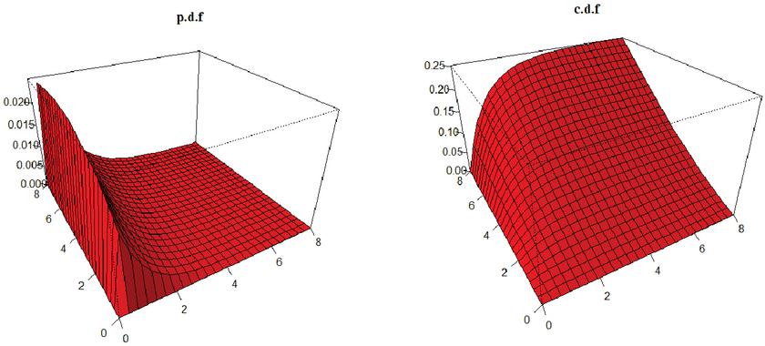
Figure 1 Plot of FGMBL distribution for ${\theta }_1=0.8$, ${\alpha }_1=0.3$, ${\theta }_2=0.1$, ${\alpha }_2=0.3$ and $\tau =0.9$.

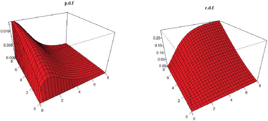
Figure 2 Plot of FGMBL distribution for ${\theta }_1$= 0.8, ${\alpha }_1=0.3$, ${\theta }_2=0.1$, ${\alpha }_2=0.3$ and $\tau =-0.9$.

4 Some Properties of FGM Bivariate Lindley Distribution

In this Section, we have derived some important statistical properties of FGMBL distribution, such as the conditional distribution, moment generating function, and positive quadrant dependence.

4.1 Conditional Distribution

The conditional c.d.f of X given Y $=$ y of FGMBL distribution is given by

$F_{X/Y}(x/y)=$	$\left(1-\tau [{\displaystyle \frac{2({\theta }_2+{\alpha }_2+{\alpha }_2{\theta }_{2}y)}{({\theta }_2+{\alpha }_2)}}{e}^{-{\theta }_{2}y}-1]\right)$
	$\mathrm{\hspace{1em}}\left(1-{\displaystyle \frac{({\theta }_1+{\alpha }_1+{\alpha }_1{\theta }_{1}x)}{({\theta }_1+{\alpha }_1)}}{e}^{-{\theta }_{1}x}\right)$
	$\mathrm{\hspace{1em}}+\tau \left({\displaystyle \frac{2({\theta }_2+{\alpha }_2+{\alpha }_2{\theta }_{2}y)}{({\theta }_2+{\alpha }_2)}}{e}^{-{\theta }_{2}y}-1\right)$
	$\mathrm{\hspace{1em}}\left(1-{\displaystyle \frac{{({\theta }_1+{\alpha }_1+{\alpha }_1{\theta }_{1}x)}^2}{{({\theta }_1+{\alpha }_1)}^2}}{e}^{-2{\theta }_{1}x}\right),$

and the corresponding p.d.f is given as

$f_{X/Y}\left(x/y\right)=$	${\displaystyle \frac{{\theta }_1^2\left(1+{\alpha }_{1}x\right)e^{-{\theta }_{1}x}}{\left({\theta }_1+{\alpha }_1\right)}}[1+\tau ({\displaystyle \frac{2\left({\theta }_1+{\alpha }_1+{\alpha }_1{\theta }_{1}x\right)}{\left({\theta }_1+{\alpha }_1\right)}}{e}^{-{\theta }_{1}x}-1).$
	$\mathrm{\hspace{1em}}({\displaystyle \frac{2\left({\theta }_2+{\alpha }_2+{\alpha }_2{\theta }_{2}y\right)}{\left({\theta }_2+{\alpha }_2\right)}}{e}^{-{\theta }_{2}y}-1)].$	(14)

Next the conditional expectation of X given $Y=y$ is obtained as

$E[X/Y=y]$	$={\displaystyle \frac{1}{{\theta }_1\left({\theta }_1+{\alpha }_1\right)}}[2\alpha {}_1+\theta {}_1-\tau ({\displaystyle \frac{2\left({\theta }_2+{\alpha }_2+{\alpha }_2{\theta }_{2}y\right)}{\left({\theta }_2+{\alpha }_2\right)}}{e}^{-{\theta }_{2}y}-1).$
	$\mathrm{\hspace{1em}}\left({\displaystyle \frac{3{\alpha }_1^2+6{\alpha }_1{\theta }_1+2{\theta }_1^2}{4\left({\theta }_1+{\alpha }_1\right)}}\right)].$	(15)

Similarly, we can derive the expressions of $F_{Y/X}(y/x)$, $f_{Y/X}(y/x)$ and E[Y/X $=$ x].

4.2 Moment Generating Function

Let (X,Y) be a two-dimensional random variable with joint p.d.f $f_{(X,Y)}(x,y)$, then the moment generating function (m.g.f) of (X,Y) is defined as

$M_{(X,Y)}(t_1,t_2)$	$=E(e^{t_{1}x}{e}^{t_{2}y})$
	$={\displaystyle {\int }_0^{\mathrm{\infty }}}{\displaystyle {\int }_0^{\mathrm{\infty }}}{e}^{t_{1}x}{e}^{t_{2}y}{f}_{(XY)}(x,y)\mathit{d}y\mathit{d}x,$	(16)

where $(t_1,t_2)$ are real parameters.

Using (4.2) and (3), the m.g.f of FGMBL distribution is obtained as

$$M_{(X,Y)}(t_1,t_2)=M+\tau \prod _{i=1}^2{K}_i({\theta }_i,{\alpha }_i,t_i),$$

(17)

where

$M$	$={\displaystyle \frac{{\theta }_1^2({\theta }_1-t_1-{\alpha }_1)}{({\theta }_1+{\alpha }_1){({\theta }_1-t_1)}^2}}{\displaystyle \frac{{\theta }_2^2({\theta }_2-t_2-{\alpha }_2)}{({\theta }_2+{\alpha }_2){({\theta }_2-t_2)}^2}},$
$K_i({\theta }_i,{\alpha }_i,t_i)$	$={\displaystyle \frac{2{\theta }_i^2}{{({\theta }_i+{\alpha }_i)}^2{(2{\theta }_i-t_i)}^3}}(t_i^2({\theta }_i+{\alpha }_i)-t_i(4{\theta }_i^2+6{\theta }_i{\alpha }_i+{\alpha }_i^2)$
	$\mathrm{\hspace{1em}}+4{\theta }_i^3+8{\alpha }_i{\theta }_i^2+4{\theta }_i{\alpha }_i^2)-{\displaystyle \frac{{\theta }_i^2({\theta }_i-t_i+{\alpha }_i)}{({\theta }_i+{\alpha }_i)(\theta i-t_i)}},i=1,2.$

4.3 Positive Quadrant Dependence(PQD)

The Positive quadrant dependence property was proposed by Lehmann (1966) [32] and in the bivariate case, it is defined as follows:

$$PQD(X,Y)=P(X>x,Y>y)\ge P(X>x)P(Y>y),\forall x,y.$$

(18)

A reverse inequality of (18) defines negative quadrant dependence (NQD). Then the following theorem gives us a condition for the FGMBL to be positive (negative) quadrant dependent.

Theorem 1 FGMBL distribution is PQD (NQD) for positive (negative) value of $\theta .$

Proof. Consider

$S(x,y)-S(x)S(y)$
$\mathrm{\hspace{1em}\hspace{1em}}=P(X>x,Y>y)-P(X>x)P(Y>y)$
$\mathrm{\hspace{1em}\hspace{1em}}={\displaystyle \frac{({\theta }_1+{\alpha }_1+{\alpha }_1{\theta }_{1}x)e^{-{\theta }_{1}x}({\theta }_2+{\alpha }_2+{\alpha }_2{\theta }_{2}y)e^{-{\theta }_{2}y}}{({\theta }_1+{\alpha }_1)({\theta }_2+{\alpha }_2)}}$
$\mathrm{\hspace{1em}\hspace{1em}}\mathit{\hspace{1em}}\tau \left(1-{\displaystyle \frac{({\theta }_1+{\alpha }_1+{\alpha }_1{\theta }_{1}x)e^{-{\theta }_{1}x}}{({\theta }_1+{\alpha }_1)}}\right)\left(1-{\displaystyle \frac{({\theta }_2+{\alpha }_2+{\alpha }_2{\theta }_{2}y)e^{-{\theta }_{2}y}}{({\theta }_2+{\alpha }_2)}}\right)$
$\mathrm{\hspace{1em}\hspace{1em}}=\tau \varphi (x,y),$	(19)

where S(x,y) be the bivariate survival function and

$\varphi (x,y)$	$={\displaystyle \frac{({\theta }_1+{\alpha }_1+{\alpha }_1{\theta }_{1}x)e^{-{\theta }_{1}x}({\theta }_2+{\alpha }_2+{\alpha }_2{\theta }_{2}y)e^{-{\theta }_{2}y}}{({\theta }_1+{\alpha }_1)({\theta }_2+{\alpha }_2)}}.$
	$\mathrm{\hspace{1em}}\left(1-{\displaystyle \frac{({\theta }_1+{\alpha }_1+{\alpha }_1{\theta }_{1}x)e^{-{\theta }_{1}x}}{({\theta }_1+{\alpha }_1)}}\right)\left(1-{\displaystyle \frac{({\theta }_2+{\alpha }_2+{\alpha }_2{\theta }_{2}y)e^{-{\theta }_{2}y}}{({\theta }_2+{\alpha }_2)}}\right)$
	$=S(x)S(y)F(x)G(y)\ge \mathrm{\hspace{0.33em}0};S(.),F(.)\ge 0,\forall x,y\ge \mathrm{\hspace{0.33em}0},$

and thus the following inequalities of $\tau \varphi (x,y)$ is given by

$$\tau \varphi (x,y)\{\begin{array}{cc}\ge \mathrm{\hspace{0.33em}0};\hfill & \tau >0,\forall x,y\ge 0,\hfill \\ \le \mathrm{\hspace{0.33em}0};\hfill & \tau <0,\forall x,y\ge 0,\hfill \end{array}$$

(20)

which implies the condition given in (20). Hence FGMBL distribution is PQD (NQD) for positive (negative) values of $\tau$. Thus FGMBL distribution possesses both positive and negative quadrant dependence.

5 Reliability Measures

In this section, we derived some important reliability characteristics of FGMBL distribution, which includes dependence stress-strength reliability, hazard rate function, Clayton-Oakes association measure, mean residual life, vitality function, totally positive of order 2 or reverse rule of order $2(T{P}_2$ or $R{R}_2)$, right-tail increasing, left-tail decreasing and mean time to failure.

5.1 Reliability for Dependence Stress and Strength

In this section, we assume that stress (Y) and strength (X) are jointly distributed according to FGMBL distribution with dependence parameter $\tau$, then the corresponding R is derived as

$R$	$=P(Y<X)={\displaystyle {\int }_0^{\mathrm{\infty }}}{\displaystyle {\int }_0^x}{f}_{(X,Y)}(x,y)dydx$
	$=1-{\displaystyle \frac{1}{({\theta }_1+{\alpha }_1)({\theta }_2+{\alpha }_2){({\theta }_1+{\theta }_2)}^3}}(\theta {}_1{}^2(({\theta }_1^2+2{\theta }_2^2+3{\theta }_1{\theta }_2$
	$\mathrm{\hspace{1em}}+({\theta }_1+3{\theta }_2){\alpha }_1){\alpha }_2+{\alpha }_1({\theta }_1{\theta }_2+{\theta }_2^2)+{\theta }_2^3+2{\theta }_1{\theta }_2^2+{\theta }_2{\theta }_1^2))$
	$\mathrm{\hspace{1em}}+\tau ({\displaystyle \frac{1}{({\theta }_1+{\alpha }_1)({\theta }_2+{\alpha }_2){({\theta }_1+{\theta }_2)}^3}}[\theta {}_1{}^2(({\theta }_2+{\alpha }_2){\theta }_1^2+(2{\theta }_2^2+3{\theta }_2{\alpha }_2$
	$\mathrm{\hspace{1em}}+2{\alpha }_1{\theta }_2+{\alpha }_1{\alpha }_2){\theta }_1+{\theta }_2^3+3{\theta }_2^2{\alpha }_2+3{\alpha }_1{\alpha }_2{\theta }_2)]$
	$\mathrm{\hspace{1em}}-{\displaystyle \frac{{\theta }_1^2}{({\theta }_1+{\alpha }_1){({\theta }_2+{\alpha }_2)}^2{(2{\theta }_2+{\theta }_1)}^3}}[(2{\theta }_2+{\theta }_1){}^3({\theta }_2+{\alpha }_2){}^2$
	$\mathrm{\hspace{1em}}+{(2{\theta }_2+{\theta }_1)}^2[{({\theta }_2+{\alpha }_2)}^2{\alpha }_1+2{\alpha }_2{\theta }_2^2+2{\theta }_2{\alpha }_2^2]+4{\alpha }_1(2{\theta }_2+{\theta }_1)$
	$\mathrm{\hspace{1em}}({\alpha }_2{\theta }_2^2+{\theta }_2{\alpha }_2^2)+6{\alpha }_1{\theta }_2^2{\alpha }_2^2]$
	$\mathrm{\hspace{1em}}-{\displaystyle \frac{2{\theta }_1^2}{({\theta }_1+{\alpha }_1)({\theta }_2+{\alpha }_2){({\theta }_1+{\theta }_2)}^3}}[(({\theta }_2+{\alpha }_2){\theta }_1^2+(2{\theta }_2^2+2{\theta }_2{\alpha }_2$
	$\mathrm{\hspace{1em}}+3{\alpha }_1{\theta }_2+{\alpha }_1{\alpha }_2){\theta }_1+{\theta }_2^3+3{\theta }_2^2{\alpha }_2+3{\alpha }_1{\alpha }_2{\theta }_2)+{\displaystyle \frac{1}{({\theta }_1+{\alpha }_1)}}$
	$\mathrm{\hspace{1em}}({({\theta }_1+{\theta }_2)}^3({\theta }_1+{\alpha }_1)({\theta }_2+{\alpha }_2)+{({\theta }_1+{\theta }_2)}^2[({\theta }_2+{\alpha }_2){\alpha }_1^2$
	$\mathrm{\hspace{1em}}+({\alpha }_2{\theta }_2+2{\theta }_1{\theta }_2+2{\theta }_1{\alpha }_2){\alpha }_1+{\theta }_1{\theta }_2{\alpha }_2]+({\theta }_1+{\theta }_2)[3{\theta }_1{\theta }_2{\alpha }_1{\alpha }_2$
	$\mathrm{\hspace{1em}}+(2{\alpha }_2{\theta }_2+{\theta }_1{\theta }_2+{\alpha }_2{\theta }_2){\alpha }_1^2]+4{\theta }_1{\theta }_2{\alpha }_1^2{\alpha }_2))]$
	$\mathrm{\hspace{1em}}+{\displaystyle \frac{2{\theta }_1^2}{{({\theta }_2+{\alpha }_2)}^2({\theta }_1+{\alpha }_1){(2{\theta }_2+{\theta }_1)}^3}}$
	$\mathrm{\hspace{1em}\hspace{1em}}[(2{\theta }_2+{\theta }_1){}^3({\theta }_2+{\alpha }_2){}^2+(2{\theta }_2+{\theta }_1){}^2$
	$\mathrm{\hspace{1em}\hspace{1em}}[{({\theta }_2+{\alpha }_2)}^2{\alpha }_1+2{\alpha }_2{\theta }_2^2+2{\theta }_2{\alpha }_2^2]+4{\alpha }_1(2{\theta }_2+{\theta }_1)({\alpha }_2{\theta }_2^2+{\theta }_2{\alpha }_2^2)$
	$\mathrm{\hspace{1em}}+6{\alpha }_1{\theta }_2^2{\alpha }_2^2-{\displaystyle \frac{1}{({\theta }_1+{\alpha }_1){(2{\theta }_2+{\theta }_1)}^2}}[{(2{\theta }_2+{\theta }_1)}^4({\theta }_1+{\alpha }_1)$
	$\mathrm{\hspace{1em}}{({\theta }_2+{\alpha }_2)}^2+({(2{\theta }_2+{\theta }_1)}^3((2{\theta }_2{\alpha }_2^2+2{\alpha }_2{\theta }_2^2)({\theta }_1$
	$\mathrm{\hspace{1em}}+{\alpha }_1)+{\alpha }_1{\theta }_1{({\theta }_2+{\alpha }_2)}^2)$
	$\mathrm{\hspace{1em}}+{\alpha }_1({\alpha }_1+{\theta }_1){({\alpha }_2+{\theta }_2)}^2)]+(2{\theta }_2+{\theta }_1){}^2[2{\theta }_2^2{\alpha }_2^2({\theta }_1$
	$\mathrm{\hspace{1em}}+{\alpha }_1)+2\alpha {}_1\theta {}_1(2{\theta }_2^2{\alpha }_2+2{\alpha }_2^2{\theta }_2)+2\alpha {}_1({\theta }_1+{\alpha }_1)(2{\theta }_2^2{\alpha }_2+2{\alpha }_2^2{\theta }_2)$
	$\mathrm{\hspace{1em}}+2{\alpha }_1^2{\theta }_1{({\theta }_2+{\alpha }_2)}^2]-(2{\theta }_2+{\theta }_1)[6{\theta }_2^2{\alpha }_2^2{\alpha }_1{\theta }_1+6{\theta }_2^2{\alpha }_2^2{\alpha }_1({\theta }_1+{\alpha }_1)$
	$\mathrm{\hspace{1em}}+6{\alpha }_1^2{\theta }_1(2{\alpha }_2{\theta }_2^2+2{\theta }_2{\alpha }_2^2)]-24{\theta }_2^2{\alpha }_2^2{\alpha }_1^2{\theta }_1]),$	(21)

when the dependence parameter $\tau =0$, then the stress-strength reliability given in (21) applies in the case where X and Y are independent. Moreover, the estimates of R can be obtained by substituting the estimates of parameters in (21).

5.2 Hazard Rate Function

Basu (1971) [9] suggested the bivariate hazard rate function of the form

$$h(x,y)=\frac{f(x,y)}{S(x,y)},$$

(22)

substituting $S(x,y)=(1-F_{X,Y}(x,y))$ from (11) and $f_{X,Y}(x,y)$ from (3) in (22), the hazard rate function of FGMBL distribution is obtained as

$h(x,y)$	$=({\displaystyle \frac{(1+{\alpha }_{1}x)(1+{\alpha }_{2}y){\theta }_1^2{\theta }_2^2}{({\theta }_1+{\alpha }_1+{\theta }_1{\alpha }_{1}x)({\theta }_2+{\alpha }_2+{\theta }_2{\alpha }_{2}y)}}).$
	$\mathrm{\hspace{1em}}{\displaystyle \frac{(1+\tau (\frac{2({\theta }_1+{\alpha }_1+{\theta }_1{\alpha }_{1}x)}{{\theta }_1+{\alpha }_1}{e}^{-{\theta }_{1}x}-1)(\frac{2({\theta }_2+{\alpha }_2+{\theta }_2{\alpha }_{2}y)-1}{{\theta }_2+{\alpha }_2}{e}^{-{\theta }_{2}y}))}{(1+\tau (1-\frac{{\theta }_1+{\alpha }_1+{\theta }_1{\alpha }_{1}x}{{\theta }_1+{\alpha }_1}{e}^{-{\theta }_{1}x})(1-\frac{{\theta }_2+{\alpha }_2+{\theta }_2{\alpha }_{2}y}{{\theta }_2+{\alpha }_2}{e}^{-{\theta }_{2}y}))}}.$	(23)

Further, Johnson and Kotz (1975) [26] defined a hazard rate function in a vector form, as shown below

$$h_V(x,y)=(\frac{-\partial lnS(x,y)}{\partial x},\frac{-\partial lnS(x,y)}{\partial y}),$$

(24)

where $S(x,y)$ is the bivariate survival function. Then the vector components of hazard rate function are given as follows

$-{\displaystyle \frac{\partial lnS(x,y)}{\partial x}}$	$={\displaystyle \frac{{\theta }_1^2(1+{\alpha }_{1}x)}{({\theta }_1+{\alpha }_1+{\theta }_1{\alpha }_{1}x)}}$
	$\mathrm{\hspace{1em}}-{\displaystyle \frac{\tau {\theta }_1^2(1+{\alpha }_{1}x)\left(1-\frac{{\theta }_2+{\alpha }_2+{\theta }_2{\alpha }_{2}y}{{\theta }_2+{\alpha }_2}{e}^{-{\theta }_{2}y}\right)e^{-{\theta }_{1}x}}{({\theta }_1+{\alpha }_1)J(x,y)}},$	(25)
$-{\displaystyle \frac{\partial lnS(x,y)}{\partial y}}$	$={\displaystyle \frac{{\theta }_2^2(1+{\alpha }_{2}y)}{({\theta }_2+{\alpha }_2+{\theta }_2{\alpha }_{2}y)}}$
	$\mathrm{\hspace{1em}}-{\displaystyle \frac{\tau {\theta }_2^2(1+{\alpha }_{2}y)\left(1-\frac{{\theta }_1+{\alpha }_1+{\theta }_1{\alpha }_{1}x}{{\theta }_1+{\alpha }_1}{e}^{-{\theta }_{1}x}\right)e^{-{\theta }_{2}y}}{({\theta }_2+{\alpha }_2)J(x,y)}}.$	(26)

where

$J(x,y)$	$=(1+\tau (1-{\displaystyle \frac{{\theta }_1+{\alpha }_1+{\theta }_1{\alpha }_{1}x}{{\theta }_1+{\alpha }_1}}{e}^{-{\theta }_{1}x})$
	$\mathrm{\hspace{1em}}(1-{\displaystyle \frac{{\theta }_2+{\alpha }_2+{\theta }_2{\alpha }_{2}y}{{\theta }_2+{\alpha }_2}}{e}^{-{\theta }_{2}y})).$

When the dependence parameter $\tau =0$ the components of $h_v(x,y)$ reduces to the marginal hazard rate function of X and Y respectively as

$$\frac{-\partial lnS(x,y)}{\partial x}=\frac{{\theta }_1^2(1+{\alpha }_{1}x)}{({\theta }_1+{\alpha }_1+{\theta }_1{\alpha }_{1}x)},$$

(27)

and

$$\frac{-\partial lnS(x,y)}{\partial y}=\frac{{\theta }_2^2(1+{\alpha }_{2}y)}{({\theta }_2+{\alpha }_2+{\theta }_2{\alpha }_{2}y)}.$$

(28)

Further, the following theorem proves that FGMBL distribution has increasing hazard rate (IHR) (decreasing hazard rate (DHR)) for positive (negative) values of $\tau$.

Theorem 1. FGMBL distribution have IHR (DHR) for positive (negative) values of $\tau$.

Proof To prove FGMBL distribution is IHR for positive values of $\tau$, it is sufficient to show that (5.2) and (5.2) are increasing functions in x and y respectively. Consider

$-{\displaystyle \frac{\partial lnS(x,y)}{\partial x}}$	$=-{\displaystyle \frac{\partial }{\partial x}}ln({\overline{F}}_X{\overline{G}}_Y[1+\tau F_X{G}_y]),\text{where}\overline{F}=1-F$
	$=-{\displaystyle \frac{\partial }{\partial x}}ln{\overline{F}}_X-{\displaystyle \frac{\partial }{\partial x}}ln{\overline{G}}_Y-{\displaystyle \frac{\partial }{\partial x}}ln(1+\tau F_X{G}_Y)$
	$=h_X[1-{({\overline{F}}_X^{-1}[{(\tau G_Y)}^{-1}+1]-1)}^{-1}],$

where $h_X$ is the hazard rate function of X given in (27) distribution. For $0\le \tau \le 1$, ${\tau }^{-1}\ge 1$ which implies $({(\tau G_Y)}^{-1}+1)>1$, because ${(G_Y)}^{-1}\ge 1$. Therefore ${[1-{({\overline{F}}_X)}^{-1}[{(\tau G_Y)}^{-1}+1]-1)}^{-1}]$ is positive increasing function in x because $F_x$ is an increasing function in x. Further, the $h_X$ is an increasing function in x. Hence $-\frac{\partial lnS(x,y)}{\partial x}$ is an increasing function in x. In a Similar way, we can prove that FGMBL distribution is DFR for negative values of $\tau$.

5.3 The Clayton-Oakes Association Measure

[40] defined the association measure for bivariate survival function as

$\theta (x,y)={\displaystyle \frac{\overline{F}{\overline{F}}_{(12)}}{{\overline{F}}_{(1)}{\overline{F}}_{(2)}}},$

where $\overline{F}=\overline{F}(x,y)$ is the survival function , ${\overline{F}}_{(12)}=\frac{{\partial }^2\overline{F}(x,y)}{\partial x\partial y}$, ${\overline{F}}_{(1)}=\frac{\partial }{\partial x}\overline{F}(x,y)$ and ${\overline{F}}_{(2)}=\frac{\partial }{\partial y}\overline{F}(x,y)$.

Clayton (1978) [14] obtained the above association measure, deriving from Cox’s model, in a study of association between the life spans of fathers and their sons, as

$\theta (x,y)={\displaystyle \frac{r(x|Y=y)}{h_1(x,y)}}=1-{\displaystyle \frac{\frac{\partial }{\partial y}{h}_1(x,y)}{h_1(x,y)h_2(x,y)}}=1-{\displaystyle \frac{\frac{\partial }{\partial x}{h}_2(x,y)}{h_1(x,y)h_2(x,y)}},$

where $h_1(x,y)=-\frac{\partial }{\partial x}ln\overline{F}(x,y)$ is the hazard rate of X given $Y>y$. Similarly $h_2(x,y)=-\frac{\partial }{\partial y}ln\overline{F}(x,y)$ is the hazard rate of Y given $X>x$. It can be proved that X and Y are independent iff $\theta (x,y)=1$.

Harris (1970) [24] suggested the following definition of right corner set increasing.

Definition 1. The random variable (X,Y) with p.d.f $f_{(X,Y)}(x,y)$ is said to be right corner set increasing (RCSI) if $P(X>x,Y>y|X>x^{{}^{\prime }},Y>y^{{}^{\prime }})$ is increasing in $x^{{}^{\prime }}$ and $y^{{}^{\prime }}$ $\forall$ x,y. The opposite inequality is applicable for left corner set decreasing (LCSD).

Remark 1. Shaked (1977) [45] shown that the following results equivalent to: (i) (X,Y) is RCSI, (ii) $\frac{\partial }{\partial y}{h}_1(x,y)$ $<$ 0, (iii) $\theta (x,y)$ $>$ 1.

Remark 2. It has been shown by Shaked (1977) [45] that if $f_{(X,Y)}(x,y)$ is $T{P}_2$, then $r(x|Y=y)$ is decreasing in y and (X, Y ) is RCSI.

Therefore the association measure for FGMBL distribution is obtained as

$\theta (x,y)=1+{\displaystyle \frac{\left(\frac{\tau e^{-{\theta }_{1}x}{\theta }_1^2(1+{\alpha }_{1}x)e^{-{\theta }_{2}y}{\theta }_2^2(1+{\alpha }_{2}y)}{({\theta }_1+{\alpha }_1)({\theta }_2+{\alpha }_2)}\right)}{(1+\tau F_X(x)G_Y(y))){}^{2}h{}_1(x,y)h{}_2(x,y)}},$

(29)

where $h_1(x,y)$ and $h_2(x,y)$ are the vector components of hazard function X given Y$>$y and Y given X$>$x defined in (5.2) and (5.2) respectively and $F_X(x)$ and $G_Y(y)$ are defined in (10) and (11) respectively. It is clear from (29) that $\theta (x,y)>(<)1$ whenever $\tau >(<)$ 0. Hence (X,Y) is right corner set increasing when $\tau >$ 0.

5.4 Mean Residual Life

Bivariate mean residual life (m.r.l) function suggested by Shanbhag and Kotz (1987) [46] is of the form

$$r(x,y)=(r_1(x,y),r_2(x,y)),$$

(30)

where

$$r_1(x,y)=E(X-x|X\ge x,Y\ge y),$$

(31)

and

$$r_2(x,y)=E(Y-y|X\ge x,Y\ge y).$$

(32)

The expression for $r_1(x,y)$ and $r_2(x,y)$ of FGMBL distribution is obtained as

$r_1(x,y)$	$={\displaystyle \frac{\frac{({\theta }_1+2{\alpha }_1+{\theta }_1{\alpha }_{1}x)e^{-{\theta }_{1}x}}{{\theta }_1}}{({\theta }_1+{\alpha }_1+{\theta }_1{\alpha }_{1}x)e^{-{\theta }_{1}x}[1+\tau F_X(x)G_Y(y)]}}$
	$\mathrm{\hspace{1em}}+{\displaystyle \frac{\tau (1-\frac{({\theta }_1+{\alpha }_1+{\theta }_1{\alpha }_{1}x)}{{\theta }_1+{\alpha }_1}{e}^{-{\theta }_{1}x})A({\theta }_1,{\alpha }_1,x)}{({\theta }_1+{\alpha }_1+{\theta }_1{\alpha }_{1}x)e^{-{\theta }_{1}x}[1+\tau F_X(x)G_Y(y)]}},$	(33)

and

$r_2(x,y)$	$={\displaystyle \frac{\frac{({\theta }_2+2{\alpha }_2+{\theta }_2{\alpha }_{2}y)e^{-{\theta }_{2}y}}{{\theta }_2}}{({\theta }_2+{\alpha }_2+{\theta }_2{\alpha }_{2}y)e^{-{\theta }_{2}y}[1+\tau F_X(x)G_Y(y)]}}$
	$\mathrm{\hspace{1em}}+{\displaystyle \frac{\tau (1-\frac{({\theta }_2+{\alpha }_2+{\theta }_2{\alpha }_{2}y)}{{\theta }_2+{\alpha }_2}{e}^{-{\theta }_{2}y})B({\theta }_2,{\alpha }_2,y)}{{\theta }_2+{\alpha }_2+{\theta }_2{\alpha }_{2}y)e{}^{-{\theta }_{2}y}[1+\tau F_X(x)G_Y(y)]}},$	(34)

where

$A({\theta }_1,{\alpha }_1,x)$	$={\displaystyle \frac{({\theta }_1+2{\alpha }_1+{\theta }_1{\alpha }_{1}x)e^{-{\theta }_{1}x}}{{\theta }_1}}$
	$\mathrm{\hspace{1em}}-{\displaystyle \frac{({\alpha }_1^2(3+2{\theta }_{1}x)+2{\alpha }_1({\theta }_1+{\theta }_{1}x+1)+2{\theta }_1)e^{-2{\theta }_{1}x}}{4{\theta }_1({\theta }_1+{\alpha }_1)}}.$

and

$B({\theta }_2,{\alpha }_2,y)$	$={\displaystyle \frac{({\theta }_2+2{\alpha }_2+{\theta }_2{\alpha }_{2}y)e^{-{\theta }_{2}y}}{{\theta }_2}}$
	$\mathrm{\hspace{1em}}-{\displaystyle \frac{({\alpha }_2^2(3+2{\theta }_{2}y)+2{\alpha }_2({\theta }_2+{\theta }_{2}y+1)+2{\theta }_2)e^{-2{\theta }_{2}y}}{4{\theta }_2({\theta }_2+{\alpha }_2)}}$

Substituting (5.4) and (5.4) in (30), give the expression of m.r.l for FGMBL distribution.

5.5 Vitality Function

Let (X,Y) be a two-dimensional random vector with survival function S(x,y), then the bivariate vitality function proposed by Sankaran and Nair (1991) [43] is given by

$$\mathbf{\text{V}}(x,y)=(V_1(x,y),V_2(x,y)),$$

(35)

where

$V_1(x,y)$	$=E[X|X\ge x,Y\ge y],$	(36)
$V_2(x,y)$	$=E[Y|X\ge x,Y\ge y],$	(37)

where X and Y represents the life time of a two-component system and $V_1(x,y)$ measures the expected life time of first component given that first component survived at age x and second component survived at age y. A similar interpretation can be given to $V_2(x,y)$.

Further, the bivariate vitality function $V_i(x,y)$ is related to the mean residual life function $r_i(x,y)$ with the following relation as

$$V_i(x,y)=x+r_i(x,y),i=1,2.$$

(38)

$V_1(x,y)$ and $V_2(x,y)$ of FGMBL distribution is obtained as

$V_1(x,y)$	$=x+{\displaystyle \frac{\frac{({\theta }_1+2{\alpha }_1+{\theta }_1{\alpha }_{1}x)e^{-{\theta }_{1}x}}{{\theta }_1}}{({\theta }_1+{\alpha }_1+{\theta }_1{\alpha }_{1}x)e^{-{\theta }_{1}x}[1+\tau F_X(x)G_Y(y)]}}$
	$\mathrm{\hspace{1em}}+{\displaystyle \frac{\tau (1-\frac{({\theta }_1+{\alpha }_1+{\theta }_1{\alpha }_{1}x)}{{\theta }_1+{\alpha }_1}{e}^{-{\theta }_{1}x})A({\theta }_1,{\alpha }_1,x)}{({\theta }_1+{\alpha }_1+{\theta }_1{\alpha }_{1}x)e^{-{\theta }_{1}x}[1+\tau F_X(x)G_Y(y)]}},$	(39)

and

$V_2(x,y)$	$=y+{\displaystyle \frac{\frac{({\theta }_2+2{\alpha }_2+{\theta }_2{\alpha }_{2}y)e^{-{\theta }_{2}y}}{{\theta }_2}}{({\theta }_2+{\alpha }_2+{\theta }_2{\alpha }_{2}y)e^{-{\theta }_{2}y}[1+\tau F_X(x)G_Y(y)]}}$
	$\mathrm{\hspace{1em}}+{\displaystyle \frac{\tau (1-\frac{({\theta }_2+{\alpha }_2+{\theta }_2{\alpha }_{2}y)}{{\theta }_2+{\alpha }_2}{e}^{-{\theta }_{2}y})B({\theta }_2,{\alpha }_2,y)}{{\theta }_2+{\alpha }_2+{\theta }_2{\alpha }_{2}y)e{}^{-{\theta }_{2}y}[1+\tau F_X(x)G_Y(y)]}},$	(40)

where $A({\theta }_1,{\alpha }_1,x)$ and $B({\theta }_2,{\alpha }_2,y)$ are defined in Section (5.4). Hence the vitality function of FGMBL distribution can be obtained by substituting (5.5) and (5.5) in (35).

5.6 Totally Positive of Order 2 or Reverse Rule of Order 2 $(T{P}_2$ or $R{R}_2)$

Let (X,Y) be a two dimensional continuous random variable with joint p.d.f $f_{(X,Y)}(x,y)$ is said to be $T{P}_2$ or $R{R}_2$ if

$$f(x,y)f(u,v)\ge (\le )f(x,v)f(u,y),x<u,y<v.$$

(41)

Then the local dependence function of (X,Y) is defined as

$r_f(x,y)$	$={\displaystyle \frac{{\partial }^2}{\partial x\partial y}}ln{f}_{(X,Y)}(x,y)$
	$={\displaystyle \frac{4\tau \frac{{\theta }_1^2{\theta }_2^2(1+{\alpha }_{1}x)(1+{\alpha }_{2}y)}{({\theta }_1+{\alpha }_1)({\theta }_2+{\alpha }_2)}{e}^{-{\theta }_{1}x-{\theta }_{2}y}}{{(1+\tau (2\frac{({\theta }_1+{\alpha }_1+{\theta }_1{\alpha }_{1}x)}{{\theta }_1+{\alpha }_1}{e}^{-{\theta }_{1}x}-1)(2\frac{({\theta }_2+{\alpha }_2+{\theta }_2{\alpha }_{2}y)}{{\theta }_2+{\alpha }_2}{e}^{-{\theta }_{2}y}-1))}^2}}.$	(42)

which is $\ge (\le )\mathrm{\hspace{0.33em}0}\text{according as}\tau \ge (\le )\mathrm{\hspace{0.33em}0}.\text{Thus}{f}_{(X,Y)}(x,y)isT{P}_2(R{R}_2)$ if $\tau \ge (\le )0$.

The following results are applicable to FGMBL distribution due to Shaked (1977) [45].

Remark 3. If FGMBL distribution is $T{P}_2(R{R}_2)$, then

1. The conditional failure rate of X given $Y=y(r(x|Y=y))$ is decreasing (increasing) in y.

2. The conditional failure rate of X given $Y>y$ is decreasing (increasing) in y.

3. The mean residual life function of X given $Y>y$ is increasing (decreasing) in y.

5.7 Right Tail Increasing and Left Tail Decreasing

Let (X,Y) be a bivariate random vector with c.d.f $F_{(X,Y)}(x,y)$ and Y is right-tail increasing (RTI) in X if

$RTI(Y|X)=P(Y>y|X>x)={\displaystyle \frac{{\overline{F}}_{(X,Y)}(x,y)}{{\overline{F}}_X(x)}}\uparrow x\forall y,$

where ${\overline{F}}_{(X,Y)}(x,y)=1-F_{(X,Y)}(x,y)and{\overline{F}}_X(x)=1-F(x).$

For FGMBL distribution,

$P(Y>y|X>x)$	$={\displaystyle \frac{({\theta }_2+{\alpha }_2+{\theta }_2{\alpha }_{2}y)}{{\theta }_2+{\alpha }_2}}{e}^{-{\theta }_{2}y}$
	$\mathrm{\hspace{1em}}(1+\tau (1-{\displaystyle \frac{({\theta }_1+{\alpha }_1+{\theta }_1{\alpha }_{1}x)}{{\theta }_1+{\alpha }_1}}{e}^{-{\theta }_{1}x}).$
	$\mathrm{\hspace{1em}}(1-{\displaystyle \frac{({\theta }_2+{\alpha }_2+{\theta }_2{\alpha }_{2}y)}{{\theta }_2+{\alpha }_2}}{e}^{-{\theta }_{2}y})),$	(44)

it is clear that $P(Y>y|X>x)>1$ for $\tau >0$ which implies $RTI(Y|X).$ Similarly, Y is left-tail decresing (LTD) in X if

$LTD(Y|X)=P(Y\le y|X\le x)={\displaystyle \frac{F_{(X,Y)}(x,y)}{F_X(x)}}\downarrow x\forall y.$

For FGMBL distribution,

$P(Y\le y|X\le x)$
$\mathrm{\hspace{1em}\hspace{1em}}=\left(1-{\displaystyle \frac{({\theta }_2+{\alpha }_2+{\theta }_2{\alpha }_{2}y)}{{\theta }_2+{\alpha }_2}}{e}^{-{\theta }_{2}y}\right).$
$\mathrm{\hspace{1em}\hspace{1em}}\mathit{\hspace{1em}}(1+\tau {\displaystyle \frac{({\theta }_1+{\alpha }_1+{\theta }_1{\alpha }_{1}x)({\theta }_2+{\alpha }_2+{\theta }_2{\alpha }_{2}y)}{({\theta }_1+{\alpha }_1)({\theta }_2+{\alpha }_2)}}{e}^{-{\theta }_{1}x-{\theta }_{2}y}),$	(46)

it is observed from the expression in (5.7) that $P(Y\le |X\le x)<1$ for $\tau <0$ which implies $LTD(Y|X).$

5.8 Mean Time To Failure

Let (X,Y) be a two-dimensional random variable with joint survival function $S(x,y)$, then the mean time to faliure is defined as

$MTTF={\displaystyle {\int }_{{\mu }_1}^{\mathrm{\infty }}}{\displaystyle {\int }_{{\mu }_2}^{\mathrm{\infty }}}S(x,y)\mathit{d}y\mathit{d}x.$

(47)

Using (47) the MTTF of FGMBL distribution is obtained as

$MTTF$	$={\displaystyle \frac{({\theta }_1+2{\alpha }_1)({\theta }_2+2{\alpha }_2)}{{\theta }_1{\theta }_2({\theta }_1+{\alpha }_1)({\theta }_2+{\alpha }_2)}}+\tau \left({\displaystyle \frac{2{\theta }_1^2+6{\theta }_1{\alpha }_1+3{\alpha }_1^2}{4{\theta }_1({\theta }_1+{\alpha }_1)}}\right).$
	$\mathrm{\hspace{1em}}\left({\displaystyle \frac{2{\theta }_2^2+6{\theta }_2{\alpha }_2+3{\alpha }_2^2}{4{\theta }_2({\theta }_2+{\alpha }_2)}}\right).$	(48)

6 Parameter Estimation

In this section, we considered three different estimation procedures which includes, maximum likelihood estimation (MLE), inference function margin (IFM) and semi-parametric (SP) method for estimating the model parameters and reliability.

6.1 Maximum Likelihood Estimation

Consider the random sample $(x_i,y_i),i=1,2,\mathrm{\dots },n$ of size n drawn from the FGMBL distribution, then the log-likelihood function is given as

$logL(\mathrm{\Theta })$	$=2nln({\theta }_1)+2nln({\theta }_2)-nln({\theta }_1+{\alpha }_1)-nln({\theta }_2+{\alpha }_2)$
	$\mathrm{\hspace{1em}}+{\displaystyle \sum _{i=1}^n}ln(1+\tau ({\displaystyle \frac{2({\theta }_1+{\alpha }_1+{\alpha }_1{\theta }_1{x}_i)}{{\theta }_1+{\alpha }_1}}{e}^{-{\theta }_1{x}_i}-1)$
	$\mathrm{\hspace{1em}}({\displaystyle \frac{2({\theta }_2+{\alpha }_2+{\alpha }_2{\theta }_2{y}_i)}{{\theta }_2+{\alpha }_2}}{e}^{-{\theta }_2{y}_i}-1)),$	(49)

where $\mathrm{\Theta }$ = (${\theta }_1,{\alpha }_1,{\theta }_2,{\alpha }_2,\tau$).

The normal equations of log-likelihood function are given as

${\displaystyle \frac{\partial logL(\mathrm{\Theta })}{\partial {\theta }_1}}$	$={\displaystyle \frac{2n}{{\theta }_1}}-{\displaystyle \frac{n}{{\theta }_1+{\alpha }_1}}-{\displaystyle \sum _{i=1}^n}{x}_i$
	$\mathrm{\hspace{1em}}+{\displaystyle \sum _{i=1}^n}\tau [{\displaystyle \frac{2({\theta }_2+{\alpha }_2+{\theta }_2{\alpha }_2{y}_i)}{{\theta }_2+{\alpha }_2}}{e}^{-{\theta }_2{y}_i}-1]D({\theta }_1,{\alpha }_2,x_i)=0,$	(50)
${\displaystyle \frac{\partial logL(\mathrm{\Theta })}{\partial {\theta }_2}}$	$={\displaystyle \frac{2n}{{\theta }_2}}-{\displaystyle \frac{n}{{\theta }_2+{\alpha }_2}}-{\displaystyle \sum _{i=1}^n}{y}_i$
	$\mathrm{\hspace{1em}}+{\displaystyle \sum _{i=1}^n}\tau [{\displaystyle \frac{2({\theta }_1+{\alpha }_1+{\theta }_1{\alpha }_1{x}_i)}{{\theta }_1+{\alpha }_1}}{e}^{-{\theta }_1{x}_i}-1]D({\theta }_2,{\alpha }_2,y_i)=0,$	(51)
${\displaystyle \frac{\partial logL(\mathrm{\Theta })}{\partial {\alpha }_1}}$	$=-{\displaystyle \frac{n}{{\theta }_1+{\alpha }_1}}+{\displaystyle \sum _{i=1}^n}{\displaystyle \frac{x_i}{1+{\alpha }_1{x}_i}}$
	$\mathrm{\hspace{1em}}+{\displaystyle \sum _{i=1}^n}\tau [{\displaystyle \frac{2({\theta }_2+{\alpha }_2+{\theta }_2{\alpha }_2{y}_i)}{{\theta }_2+{\alpha }_2}}{e}^{-{\theta }_2{y}_i}-1]Q({\theta }_1,{\alpha }_2,x_i)=0,$	(52)
${\displaystyle \frac{\partial logL(\mathrm{\Theta })}{\partial {\alpha }_2}}$	$=-{\displaystyle \frac{n}{{\theta }_2+{\alpha }_2}}+{\displaystyle \sum _{i=1}^n}{\displaystyle \frac{y_i}{1+{\alpha }_2{y}_i}}$
	$\mathrm{\hspace{1em}}+{\displaystyle \sum _{i=1}^n}\tau [{\displaystyle \frac{2({\theta }_1+{\alpha }_1+{\theta }_1{\alpha }_2{x}_i)}{{\theta }_1+{\alpha }_1}}{e}^{-{\theta }_1{x}_i}-1]Q({\theta }_2,{\alpha }_2,Y_i)=0,$	(53)

and

${\displaystyle \frac{\partial logL(\mathrm{\Theta })}{\partial \tau }}$	$={\displaystyle \sum _{i=1}^n}\left[{\displaystyle \frac{2({\theta }_1+{\alpha }_1+{\theta }_1{\alpha }_1{x}_i)}{{\theta }_1+{\alpha }_1}}{e}^{-{\theta }_1{x}_i}-1\right]$
	$\mathrm{\hspace{1em}}\left[{\displaystyle \frac{2({\theta }_2+{\alpha }_2+{\theta }_2{\alpha }_2{y}_i)}{{\theta }_2+{\alpha }_2}}{e}^{-{\theta }_2{y}_i}-1\right]{\displaystyle \frac{1}{L(x_i,y_i)}}=0,$	(54)

where

$D({\theta }_1,{\alpha }_1,x_i)$	$={\displaystyle \frac{((1+{\alpha }_1{x}_i)({\theta }_1+{\alpha }_1)-({\theta }_1+{\alpha }_1+{\theta }_1{\alpha }_1{x}_i)({\theta }_1({\theta }_1+{\alpha }_1)-1))2e^{-{\theta }_1{x}_i}}{{({\theta }_1+{\alpha }_1)}^{2}L(x_i,y_i)}},$
$D({\theta }_2,{\alpha }_2,y_i)$	$={\displaystyle \frac{((1+{\alpha }_2{y}_i)({\theta }_2+{\alpha }_2)-({\theta }_2+{\alpha }_2+{\theta }_2{\alpha }_2{y}_i)({\theta }_2({\theta }_2+{\alpha }_2)-1))2e^{-{\theta }_2{y}_i}}{{({\theta }_2+{\alpha }_2)}^{2}L(x_i,y_i)}},$
$Q({\theta }_1,{\alpha }_1,x_i)$	$={\displaystyle \frac{((1+{\theta }_1{x}_i)({\theta }_1+{\alpha }_1)-({\theta }_1+{\alpha }_1+{\theta }_1{\alpha }_1{x}_i))2e^{-{\theta }_1{x}_i}}{{({\theta }_1+{\alpha }_1)}^{2}L(x_i,y_i)}},$
$Q({\theta }_2,{\alpha }_2,y_i)$	$={\displaystyle \frac{((1+{\theta }_2{y}_i)({\theta }_2+{\alpha }_2)-({\theta }_2+{\alpha }_2+{\theta }_2{\alpha }_2{y}_i))2e^{-{\theta }_2{y}_i}}{{({\theta }_2+{\alpha }_2)}^{2}L(x_i,y_i)}},$
$L(x_i,y_i)$	$=[1+\tau (2{\displaystyle \frac{({\theta }_1+{\alpha }_1+{\theta }_1{\alpha }_1{x}_i)}{{\theta }_1+{\alpha }_1}}{e}^{-{\theta }_1{x}_i}-1)$
	$\mathrm{\hspace{1em}}(2{\displaystyle \frac{({\theta }_2+{\alpha }_2+{\theta }_2{\alpha }_2{y}_i)}{{\theta }_2+{\alpha }_2}}{e}^{-{\theta }_2{y}_i}-1)].$

The likelihood Equations (6.1)–(6.1) are not in explicit form and cannot be solved analytically. We solve the likelihood equations numerically by using the Nelder-Mead optimization algorithm. Under invariance property, the MLE $\widehat{R}$ may be obtained by replacing ${\theta }_1,{\theta }_2,\alpha {}_1,{\alpha }_2$ and $\tau$ by their MLE’s ${\widehat{\theta }}_1,{\widehat{\theta }}_2,{\widehat{\alpha }}_1,{\widehat{\alpha }}_2,$ and $\widehat{\tau }$, respectively, in (21).

6.2 Estimation by Inference Function Margin

Xu (1996) [54] and Joe (2005) [25] proposed the inference margin method for a two-stage estimation process in which we estimate the marginal distribution separately in the first stage.

$${\mathrm{\ell }}_1=\sum _{i=1}^{n}lnf(x_i,{\delta }_1);{\mathrm{\ell }}_2=\sum _{i=1}^{n}lng(y_i,{\delta }_2),$$

(55)

where ${\delta }_1$ and ${\delta }_2$ be the parameters of marginal distributions.

Next, according to the previous step, the joint density is optimized by using the dependence parameter $\tau$ by considering the ML estimates obtained in the previous step of the marginals $\widehat{F}(x_i,{\delta }_1)$ and $\widehat{G}(y_i,{\delta }_2)$. Then the log-likelihood function of stress random sample (Y) and strength random sample (X) from two-parameter Lindley distribution are separately obtained as

${\mathrm{\ell }}_1=2nln({\theta }_1)-nln({\theta }_1+{\alpha }_1)+{\displaystyle \sum _{i=1}^n}ln(1+{\alpha }_1{x}_i)-{\theta }_1{\displaystyle \sum _{i=1}^n}{x}_i,$

${\mathrm{\ell }}_2=2nln({\theta }_2)-nln({\theta }_2+{\alpha }_2)+{\displaystyle \sum _{i=1}^n}ln(1+{\alpha }_2{y}_i)-{\theta }_2{\displaystyle \sum _{i=1}^n}{y}_i.$

The MLEs (${\widehat{\theta }}_1$, ${\widehat{\alpha }}_1$, ${\widehat{\theta }}_2$, ${\widehat{\alpha }}_2$) are obtained by solving simultaneously the log-likelihood equations

${{\displaystyle \frac{\partial {\mathrm{\ell }}_1}{\partial {\theta }_1}}|}_{{\theta }_1={\widehat{\theta }}_1}=0,{{\displaystyle \frac{\partial {\mathrm{\ell }}_1}{\partial {\alpha }_1}}|}_{{\alpha }_1={\widehat{\alpha }}_1}=0,{{\displaystyle \frac{\partial {\mathrm{\ell }}_2}{\partial {\theta }_2}}|}_{{\theta }_2={\widehat{\theta }}_2}=0,{{\displaystyle \frac{\partial {\mathrm{\ell }}_2}{\partial {\alpha }_2}}|}_{{\alpha }_2={\widehat{\alpha }}_2}=0,$

then

$\widehat{F}(x)$	$=1-{\displaystyle \frac{{\widehat{\theta }}_1+{\widehat{\alpha }}_1+{\widehat{\alpha }}_1{\widehat{\theta }}_{1}x}{{\widehat{\theta }}_1+{\widehat{\alpha }}_1}}{e}^{-{\widehat{\theta }}_{1}x}\mathit{\hspace{1em}}\text{and}$
$\widehat{G}(y)$	$=1-{\displaystyle \frac{{\widehat{\theta }}_2+{\widehat{\alpha }}_2+{\widehat{\alpha }}_2{\widehat{\theta }}_{1}y}{{\widehat{\theta }}_2+{\widehat{\alpha }}_2}}{e}^{-{\widehat{\theta }}_{2}y}.$

and considering the previous step, the IFM estimate of a FGMBL distribution is defined as

$${\mathrm{\ell }}_{IFM}=\sum _{i=1}^{n}ln\left(1+\tau (1-2\widehat{F}(x))(1-2\widehat{G}(y))\right).$$

(58)

The log-likelihood equation with respect to $\tau$ is given as

$$\frac{\partial \mathrm{\ell }}{\partial \tau }=\sum _{i=1}^n(\frac{p(x_i,y_i)}{1+\tau p(x_i,y_i)})=0,$$

(59)

where

$p(x_i,y_i)$	$=\left({\displaystyle \frac{2({\widehat{\theta }}_1+{\widehat{\alpha }}_1+{\widehat{\alpha }}_1{\widehat{\theta }}_1{x}_i)}{{\widehat{\theta }}_1+{\widehat{\alpha }}_1}}{e}^{-{\widehat{\theta }}_1{x}_i}-1\right)$
	$\mathrm{\hspace{1em}}\left({\displaystyle \frac{2({\widehat{\theta }}_2+{\widehat{\alpha }}_2+{\widehat{\alpha }}_2{\widehat{\theta }}_2{y}_i)}{{\widehat{\theta }}_2+{\widehat{\alpha }}_2}}{e}^{-{\widehat{\theta }}_2{y}_i}-1\right).$

The likelihood equation of $\tau$ in (59) is not in closed form and cannot be solved analytically. We solved likelihood equation numerically by using Nelder-Mead optimization algorithm in R-software. Under invariance property, the MLE $\widehat{R}$ may be obtained by replacing ${\theta }_1,{\theta }_2,\alpha {}_1,{\alpha }_2$ and $\tau$ by their MLE’s ${\widehat{\theta }}_1,{\widehat{\theta }}_2,{\widehat{\alpha }}_1,{\widehat{\alpha }}_2,$ and $\widehat{\tau }$, respectively, in (21).

6.3 Estimation by Semi-parametric Method

Kim et al. (2007) [28] proposed the semi-parametric estimation method. Which involves in estimating the model parameters of the marginal distributions non-parametrically by using sample empirical distributions by transforming the observations into pseudo-observations. The empirical distribution function is defined as follows

$${\tilde{F}}_i(x)=\frac{{\sum }_{j=1}^{n}I(X_{i,j}\le x_i)}{n+1};i=1,2,$$

(60)

where I is the indicator function.

Then, $\tau$ is estimated by the maximizer of the pseudo log-likelihood,

$${\mathrm{\ell }}_{SP}=\sum _{i=1}^{n}ln\left[c(\tilde{F}(x),\tilde{G}(y);\tau )\right],$$

(61)

by considering (61), the log-likelihood function of FGMBL distribution is given by

$${\mathrm{\ell }}_{SP}=\sum _{i=1}^{n}ln\left[1+\tau (1-2\tilde{F}(x)(1-2\tilde{G}(y)))\right].$$

(62)

There is no closed-form expression for the MLE $\widehat{\tau }$ and hence it is solved numerically by using Nelder-Mead optimization algorithm.

7 Asymptotic Confidence Interval

In this section, we propose the asymptotic confidence interval of model parameter $\mathrm{\Theta }$=(${\theta }_1$,${\alpha }_1$,${\theta }_2$,${\alpha }_2$,$\tau$) using ML, IFM, and SP methods. For this, we first obtain the observed Fishers information matrix under MLE is given as

where H is the Hessian matrix.

Our interest is to develop the confidence interval for the dependence parameter $\tau$, then the hessian matrix under IFM and SP methods is obtained as

$$H=\frac{{\partial }^2\mathrm{\ell }}{\partial {\tau }^2}.$$

(64)

Hence the $100(1-\gamma )\%$ confidence interval for $\tau$ can be obtained as

$$\widehat{\tau }\pm Z_{\gamma /2}\sqrt{Var(\widehat{\tau })},$$

where $Var(\widehat{\tau })$ is the diagonal entries of the inverse of observed Fisher information matrix and $Z_{\gamma /2}$ is the upper percentile of standard normal variate.

8 Simulation Study

A numerical study is performed to assess the performance of stress-strength reliability R and the dependence parameter $\tau$ given in the previous Sections. The main aim of this study is to assess the variation in R in relation to the variation in the dependent parameter $\tau$. The estimate of $\tau$ using MLE in Equation (6.1), IFM in Equation (59) and SP in Equation (62) are numerically computed by with Nelder-Mead method in R software using the maxLik and copula packages. A numerical comparison of point estimates of R is carried out under MLE and IFM methods for different sample sizes based on Mean Square Error (MSE). Further, a numerical investigation of point and asymptotic confidence interval estimates of $\tau$ are performed under MLE, IFM, and SP methods for comprehensive comparison purposes. We use the following steps to generate samples $(x_i,y_i)$, i $=$ $1,2,\mathrm{\dots }n$ from FGMBL distribution with parameters ${\theta }_1,{\theta }_2,{\alpha }_1,{\alpha }_2$ and $\tau$.

1. Generate two independent random samples $u_i$ and $t_i$ for i = 1, 2,… , n, from U(0,1) distribution

Table 1 Estimates of R for different choices of parameters

n		(${\theta }_1,{\alpha }_1,$ ${\theta }_2,{\alpha }_2$) $\tau$	-0.9	-0.5	-0.1	0.1	0.5	0.9
	MLE	(0.8, 0.3, 0.1, 0.5)	0.7965	0.8041	0.8118	0.8156	0.8232	0.8308
			0.7546	0.7866	0.7922	0.7838	0.7941	0.8280
			0.0232	0.0216	0.0207	0.0202	0.0205	0.0220
		(0.7, 0.3, 0.2, 0.4)	0.7797	0.8014	0.8231	0.8439	0.8756	0.8972
			0.7120	0.8108	0.8426	0.8633	0.8694	0.8917
			0.0100	0.0167	0.0077	0.0273	0.0159	0.0057
		(0.6, 0.2, 0.3, 0.1)	0.8937	0.9119	0.9201	0.9391	0.9573	0.9755
			0.8402	0.8667	0.8802	0.9033	0.9142	0.9202
			0.0541	0.0456	0.1225	0.0222	0.0221	0.0141
50
	IFM	(0.8, 0.3, 0.1, 0.5)	0.7965	0.8041	0.8118	0.8156	0.8232	0.8308
			0.7656	0.7773	0.8015	0.7972	0.7829	0.8130
			0.2019	0.2867	0.5214	0.0662	0.0672	0.0342
		(0.7, 0.3, 0.2, 0.4)	0.7797	0.8014	0.8231	0.8439	0.8756	0.8972
			0.7068	0.8067	0.8378	0.8493	0.8570	0.8805
			0.0791	0.0758	0.0116	0.3210	0.1251	0.0288
		(0.6, 0.2, 0.3, 0.1)	0.8937	0.9119	0.9201	0.9391	0.9573	0.9755
			0.8547	0.8788	0.8924	0.9187	0.9242	0.9347
			0.0102	0.0946	0.0891	0.0151	0.0233	0.0102
	MLE	(0.8, 0.3, 0.1, 0.5)	0.7965	0.8041	0.8118	0.8156	0.8232	0.8308
			0.7716	0.7925	0.7990	0.8039	0.8161	0.8206
			0.0156	0.0150	0.0147	0.0149	0.0160	0.0177
		(0.7, 0.3, 0.2, 0.4)	0.7797	0.8014	0.8231	0.8439	0.8756	0.8972
			0.7721	0.8215	0.8548	0.8749	0.8809	0.9150
			0.0078	0.0151	0.0046	0.0044	0.0046	0.0047
		(0.6, 0.2, 0.3, 0.1)	0.8937	0.9119	0.9201	0.9391	0.9573	0.9755
			0.8578	0.8893	0.9025	0.9104	0.9242	0.9378
			0.0028	0.0060	0.0128	0.0117	0.0021	0.0025
100
	IFM	(0.8, 0.3, 0.1, 0.5)	0.7965	0.8041	0.8118	0.8156	0.8232	0.8308
			0.7604	0.7899	0.8035	0.8105	0.8279	0.8303
			0.0387	0.1723	0.0295	0.0320	0.1480	0.0289
		(0.7, 0.3, 0.2, 0.4)	0.7797	0.8014	0.8231	0.8439	0.8756	0.8972
			0.7820	0.8180	0.8465	0.8612	0.8832	0.9020
			0.0160	0.0301	0.0056	0.0291	0.0337	0.0051
		(0.6, 0.2, 0.3, 0.1)	0.8937	0.9119	0.9201	0.9391	0.9573	0.9755
			0.8758	0.8911	0.9139	0.9399	0.9342	0.9458
			0.0100	0.0127	0.0202	0.0220	0.0025	0.0098
	MLE	(0.8, 0.3, 0.1, 0.5)	0.7965	0.8041	0.8118	0.8156	0.8232	0.8308
			0.7856	0.8172	0.8267	0.8257	0.8480	0.8526
			0.0011	0.0009	0.0015	0.0006	0.0017	0.0010
		(0.7, 0.3, 0.2, 0.4)	0.7797	0.8014	0.8231	0.8439	0.8756	0.8972
			0.7906	0.8309	0.8737	0.8999	0.9032	0.9386
			0.009	0.0019	0.0004	0.0003	0.0002	0.0005
		(0.6, 0.2, 0.3, 0.1)	0.8937	0.9119	0.9201	0.9391	0.9573	0.9755
			0.8807	0.9021	0.9136	0.9213	0.9558	0.9707
			0.0013	0.0008	0.0021	0.0011	0.0009	0.0003
200
	IFM	(0.8, 0.3, 0.1, 0.5)	0.7965	0.8041	0.8118	0.8156	0.8232	0.8308
			0.7854	0.8039	0.8227	0.8372	0.8406	0.8650
			0.0021	0.0011	0.0011	0.0010	0.0021	0.0021
		(0.7, 0.3, 0.2, 0.4)	0.7797	0.8014	0.8231	0.8439	0.8756	0.8972
			0.8007	0.8282	0.8529	0.8820	0.8976	0.9250
			0.0011	0.0024	0.0015	0.0009	0.0005	0.0010
		(0.6, 0.2, 0.3, 0.1)	0.8937	0.9119	0.9201	0.9391	0.9573	0.9755
			0.8711	0.9125	0.9243	0.9447	0.9590	0.9611
			0.0016	0.0016	0.0056	0.0015	0.0011	0.0016
The values in the first row are true value for R, the values in the second row are estimates of R and the values in the third row are MSE for R.

Table 2 Estimates of $\tau$ for different choices of parameters

n		(${\theta }_1,{\alpha }_1,$ ${\theta }_2,{\alpha }_2$) $\tau$	-0.9	-0.5	-0.1	0.1	0.5	0.9
	MLE	(0.8, 0.3, 0.1, 0.5)	-0.9081	-0.4960	-0.0895	0.1450	0.5507	0.9476
			0.0229	0.0211	0.0199	0.0188	0.0137	0.0110
			1.2496	1.3762	1.4272	1.4218	1.3198	1.1859
			0.9690	0.9670	0.9490	0.9564	0.9501	0.9590
		(0.7, 0.3, 0.2, 0.4)	-0.9130	-0.5088	-0.0963	0.1147	0.5175	0.9148
			0.0127	0.0118	0.0125	0.0123	0.0115	0.0128
			1.1204	1.1452	1.2556	1.2483	1.1317	0.9705
			0.9560	0.9564	0.9522	0.9500	0.9600	0.9562
		(0.6, 0.2, 0.3, 0.1)	-0.8980	-0.4793	-0.0864	0.1111	0.4952	0.9280
			0.0126	0.0238	0.1111	0.0234	0.0122	0.0226
			0.9165	1.1655	1.1966	1.0847	1.9730	0.9665
			0.9587	0.9432	0.9521	0.9605	0.9517	0.9589
	IFM	(0.8, 0.3, 0.1, 0.5)	-0.9384	-0.4841	0.1832	0.1896	0.5090	0.9557
			0.4696	0.2999	0.1681	0.1192	0.0767	0.1006
			1.1140	1.1130	1.1010	1.0903	1.0366	0.9760
			0.9070	0.9140	0.9190	0.9060	1.0366	0.9130
50		(0.7, 0.3, 0.2, 0.4)	-0.9783	0.5390	-0.0624	0.1223	0.6360	0.9115
			0.2663	0.1473	0.0987	0.2554	0.0934	0.0769
			1.8199	1.2143	1.7092	0.7161	0.9035	0.8280
			0.9120	0.9020	0.9080	0.9100	0.9110	0.9150
		(0.6, 0.2, 0.3, 0.1)	-0.9393	-0.5648	-0.1585	0.0899	0.5218	0.9493
			0.1061	0.4563	0.1032	0.0377	0.0874	0.2061
			1.0035	1.8638	1.0670	1.8178	1.9143	1.0235
			0.9060	0.9105	0.9201	0.9280	0.9180	0.9080
	SP	(0.8, 0.3, 0.1, 0.5)	-0.9204	-0.4947	-0.1064	0.0837	0.4978	0.9355
			0.1220	0.1140	0.1110	0.1137	0.1151	0.1285
			1.1272	1.2400	1.2905	1.2943	1.2349	1.1305
			0.9180	0.9240	0.9330	0.9330	0.9280	0.9030
		(0.7, 0.3, 0.2, 0.4)	-0.9315	-0.4917	-0.0892	0.0950	0.4953	0.9038
			0.0905	0.0506	0.0894	0.0927	0.0799	0.0717
			0.9894	1.0541	1.1605	1.1599	1.0581	0.9063
			0.9060	0.9100	0.9340	0.9380	0.9350	0.9160
		(0.6, 0.2, 0.3, 0.1)	-0.9189	-0.5270	-0.1261	0.0957	0.5121	0.9289
			0.0667	0.0656	0.0826	0.0663	0.0961	0.0767
			0.8553	0.9680	1.0159	1.0203	0.9058	0.8653
			0.9120	0.9340	0.9356	0.9460	0.9210	0.9129
	MLE	(0.8, 0.3, 0.1, 0.5)	-0.9083	-0.5071	-0.0998	0.1382	0.5435	0.9456
			0.0107	0.0119	0.0106	0.0108	0.0096	0.0062
			1.0689	1.1971	1.2411	1.2270	1.1639	0.9897
			0.9720	0.9790	0.9510	0.9655	0.9655	0.9622
		(0.7, 0.3, 0.2, 0.4)	-0.9017	-0.5028	-0.0989	0.1042	0.5037	0.9028
			0.0019	0.0014	0.0013	0.0013	0.0099	0.0096
			1.0469	1.0878	1.1251	1.1239	1.0807	0.9326
			0.9617	0.9602	0.9600	0.9610	0.9730	0.9620
		(0.6, 0.2, 0.3, 0.1)	-0.8977	-0.4963	-0.0961	0.1294	0.4962	0.9077
			0.0044	0.0124	0.058	0.0118	0.0222	0.0149
			0.8431	1.0819	0.4921	1.0985	0.9730	0.8131
			0.9655	0.9587	0.9650	0.9788	0.9603	0.9605
	IFM	(0.8, 0.3, 0.1, 0.5)	-0.8539	-0.5092	-0.0953	0.1187	0.4883	0.9101
			0.1386	0.1025	0.0791	0.0702	0.0776	0.1123
			1.0689	1.0195	1.0436	1.0388	1.0112	0.9486
n		(${\theta }_1,{\alpha }_1,$ ${\theta }_2,{\alpha }_2$) $\tau$	-0.9	-0.5	-0.1	0.1	0.5	0.9
			0.9390	0.9310	0.9350	0.9250	0.9380	0.9370
100		(0.7, 0.3, 0.2, 0.4)	-0.9219	-0.4972	-0.0659	0.1168	0.5208	0.9226
			0.0582	0.0206	0.0522	0.0409	0.0306	0.0405
			0.9688	0.9870	0.9967	0.9852	0.9217	0.8046
			0.9230	0.9160	0.9100	0.9240	0.9260	0.9390
		(0.6, 0.2, 0.3, 0.1)	-0.0801	-0.4934	-0.1194	0.0958	0.5018	0.0901
			0.2436	0.0600	0.0552	0.0256	0.0574	0.0636
			0.9798	0.8915	0.9028	0.9598	0.9143	0.9598
			0.9140	0.9210	0.9302	0.9210	0.9380	0.9150
	SP	(0.8, 0.3, 0.1, 0.5)	-0.9250	-0.5006	-0.0847	0.0987	0.4949	0.9272
			0.0994	0.0909	0.0916	0.0922	0.0865	0.0875
			0.9973	1.1040	1.1561	1.1561	1.1121	1.0022
			0.9220	0.9413	0.9420	0.9470	0.9350	0.9140
		(0.7, 0.3, 0.2, 0.4)	-0.9214	-0.4971	0.1021	0.0986	0.5104	0.9200
			0.0535	0.0419	0.0364	0.0551	0.0411	0.0361
			0.9410	1.0124	1.0593	1.0573	1.0097	0.8623
			0.9190	0.9230	0.9420	0.9460	0.9490	0.9290
	SP	(0.6, 0.2, 0.3, 0.1)	-0.9090	-0.4988	-0.0944	0.1130	0.5091	0.9150
			0.0381	0.0455	0.0582	0.0232	0.0361	0.0381
			0.8025	0.9078	0.9479	0.9492	0.9058	0.7925
			0.9250	0.9450	0.9438	0.9510	0.9310	0.9270
	MLE	(0.8, 0.3, 0.1, 0.5)	-0.9041	-0.5054	-0.1046	0.1008	0.5026	0.9045
			0.0008	0.0011	0.0012	0.0014	0.0013	0.0011
			0.6653	0.7878	0.8234	0.8206	0.7755	0.6509
			0.9800	0.9810	0.9710	0.9711	0.9721	0.9715
		(0.7, 0.3, 0.2, 0.4)	-0.9068	-0.5070	-0.1093	0.1096	0.5008	0.9012
			0.0002	0.0002	0.0002	0.0002	0.0002	0.0002
			0.7238	0.8122	0.8463	0.8447	0.8109	0.7221
			0.9782	0.9782	0.9702	0.9750	0.9809	0.9110
		(0.6, 0.2, 0.3, 0.1)	-0.9011	-0.5047	-0.1084	0.1097	0.5010	0.9011
			0.0021	0.0012	0.0012	0.0013	0.0051	0.0012
			0.7135	0.8148	0.4170	0.9547	0.8407	0.6135
			0.9702	0.9658	0.9721	0.9785	0.9890	0.9702
	IFM	(0.8, 0.3, 0.1, 0.5)	-0.9099	-0.5088	-0.1024	0.1047	0.5088	0.9093
			0.0381	0.0142	0.0147	0.0055	0.0148	0.0193
			0.6867	0.7909	0.8307	0.8276	0.7937	0.6942
			0.9570	0.9560	0.9490	0.9440	0.9450	0.9390
200		(0.7, 0.3, 0.2, 0.4)	-0.9045	-0.5094	-0.1031	0.1037	0.5083	0.9060
			0.0032	0.0094	0.0163	0.0032	0.0066	0.0260
			0.6874	0.7830	0.8228	0.8220	0.7812	0.6832
			0.9340	0.9440	0.9480	0.9460	0.9380	0.9450
		(0.6, 0.2, 0.3, 0.1)	-0.9055	-0.5092	-0.1040	0.1084	0.5046	0.9055
			0.0145	0.0017	0.0169	0.0077	0.0132	0.0045
			0.6886	0.7864	0.8244	0.8327	0.7953	0.5886
			0.9260	0.9300	0.9420	0.9400	0.9340	0.9260
	SP	(0.8, 0.3, 0.1, 0.5)	-0.8979	-0.5046	-0.1093	0.1049	0.5075	0.9017
			0.0113	0.0124	0.0141	0.0052	0.0145	0.0081
			0.6836	0.7865	0.8253	0.8241	0.7879	0.6867
			0.9400	0.9590	0.9620	0.9530	0.9440	0.9290
		(0.7, 0.3, 0.2, 0.4)	-0.9040	-0.5097	-0.1017	0.1039	0.5083	0.9070
			0.0188	0.0023	0.0064	0.0136	0.0170	0.0187
			0.6892	0.7849	0.8252	0.8240	0.7841	0.7221
			0.9270	0.9400	0.9510	0.9530	0.9560	0.9110
		(0.6, 0.2, 0.3, 0.1)	-0.9077	-0.5058	-0.1031	0.1099	0.5006	0.9077
			0.0084	0.0115	0.0068	0.0068	0.0109	0.0054
			0.6866	0.7849	0.8236	0.8227	0.7851	0.5866
			0.9340	0.9490	0.9560	0.9640	0.9430	0.9340
Note: The values in the second row are MSE for $\tau$.The values in the third and fourth row is the length of confidence interval and coverage probability for $\tau$.

2. Compute $v_i$ using the equation $C(v_i|u_i)$ = $t_i$ and where $C(v_i|u_i)$ represents the conditional copula of FGMBL distrinution.

3. The simulated pairs of data, say $(x_i,y_i)$for i = 1, 2,…, n, is obtained by using the following quantiles function of Lindley distributions:

$x_i=-{\displaystyle \frac{{\theta }_1+{\alpha }_1}{{\theta }_1{\alpha }_1}}-{\displaystyle \frac{1}{{\theta }_1}}W\left[-{\displaystyle \frac{1}{{\alpha }_1}}(1-u_i)({\theta }_1+{\alpha }_1)e^{-\frac{{\theta }_1+{\alpha }_1}{{\alpha }_1}}\right],$

$i=1,2,\mathrm{\dots },n$

$y_i=-{\displaystyle \frac{{\theta }_2+{\alpha }_2}{{\theta }_2{\alpha }_2}}-{\displaystyle \frac{1}{{\theta }_2}}W\left[-{\displaystyle \frac{1}{{\alpha }_2}}(1-v_i)({\theta }_2+{\alpha }_2)e^{-\frac{{\theta }_2+{\alpha }_2}{{\alpha }_2}}\right],$

$i=1,2,\mathrm{\dots },n$

where W(.) is the Lambert’s W function.

A Monte-Carlo simulation study is performed based on the data sets generated from the FGMBL distribution for three different sets of chosen values of parameters within their range

$({\theta }_1,{\theta }_2,{\alpha }_1,{\alpha }_2)=((0.8,0.3,0.1,0.5),(0.6,0.2,0.3,0.1),(0.7,0.3,0.2,0.4))$

along with each of chosen values of the dependence parameter $\tau =(-0.9,-0.5$, $-0.1,0.1$, $0.5,0.9)$ with in the parameter space. For each case, 1000 data sets were simulated with samples sizes $n=50$, 100, and 200. The average estimate and MSE of R are given in Table 1. We computed the average estimates, MSE, length of the confidence interval (L.CI), and coverage probability (CP) for the dependence parameter $\tau$ are presented in Table 2. Further, the formula used for computing MSE, CP, and L.CI are given as follows

$$MSE=\frac{1}{n}\sum _1^n{(\widehat{\delta }-\delta )}^2,$$

(65)

where $\widehat{\delta }$ is the estimated value of $\delta$.

$$L.CI=U(\widehat{\delta })-L(\widehat{\delta }),$$

(66)

where $U(\widehat{\delta })$ and $L(\widehat{\delta })$ denote the upper and lower confidence interval of $\delta$ respectively.

$$CP=\frac{1}{n}\sum _1^n{I}_{D_i},$$

(67)

where

$$I_{D_i}=\{\begin{array}{cc}1\mathit{\hspace{1em}}\hfill & \text{if}\delta \in [L(\widehat{\delta }),U(\widehat{\delta })],\hfill \\ 0\mathit{\hspace{1em}}\hfill & \text{if}\delta \notin [L(\widehat{\delta }),U(\widehat{\delta })].\hfill \end{array}$$

(68)

It is observed from the numerical results presented in Tables 1 and 2 that

For all approaches examined, the MSEs of the estimates decrease with increase in the sample sizes. But for estimating the dependence parameter $\tau$, the MLE method performs better than the other methods.

With the increase of sample size, the length of the confidence interval (L.CI) decreases for all of the three methods considered.

coverage probability (CP) for the estimate of $\tau$ increases as sample size increases in all the considered methods and becomes close to the significance value.

With increasing sample sizes, MSEs for R estimates decreases under both MLE and IFM and MLE provides the better estimate compared to IFM based on MSEs. Further, we observed that when $\tau$ increases, R’s variation increases and vice versa. This means R and $\tau$ have a positive relationship.

9 Real Data Analysis

In this section, we analyse the data set originally reported by McGilchrist and Aisbett (1991) [36]. The data represents the recurrence time of infection for the kidney disease patients using portable dialysis equipment. Turk et al. (2017) [52] analysed the same data sets to estimate the parameters of bivariate generalized exponential distribution based on Plackett and FGM copula using MLE, IFM, and CML approaches. Recently, Ahmed and Mokhli (2020) [1] modelled this data for Bivariate General Exponential and Bivariate General Inverse Exponential distributions linked by FGM copula to estimate the parameters and stress-strength reliability R by MLE and Bayesian methods.

Let X and Y represents the first and second recurrence times, respectively. The data for the 30 patients are given as follows

$X:$	$\mathrm{}8,23,22,447,30,24,7,511,53,15,7,141,96,149,536,17,185,292,$
	$\mathrm{}22,15,152,402,13,39,12,113,132,34,2,130.$
$Y:$	$\mathrm{}16,13,28,318,12,245,9,30,196,154,333,8,38,70,25,4,117,114,$
	$\mathrm{}159,108,362,24,66,46,40,201,156,30,25,26.$

We transformed both the data sets stress (Y) and the strength (X) by taking the square root of the data and dividing it by 0.1. It is noted that the resultant data fits quite well with the proposed model.The data is relevant to the distribution based on FGM copula since the correlation between data is weak ($-\frac{1}{3}$,$\frac{1}{3}$). The correlation coefficient and test of correlation for the real data are reported in Table 3.

Table 3 The correlation coefficient and test of correlation for real data

Correlation Measure	Correlation	P-value
Pearson’s	0.09014	0.6357
Kendall’s	0.11098	0.3914

First, we investigated the validity of the Lindley distribution by fitting it to X and Y separately. The graph of empirical and theoretical c.d.f and P–P plot for Lindley with other univariate distributions are given in Figures 3 and 4, respectively. From these graph, we conclude that Lindley distribution fit these data sets well. This conclusion is also supported by the Kolmogorov-Smirnov tests, as given in Table 4.

Table 4 Goodness of fit test for Lindley distribution

	X				Y
	D (test statistic)	P-value	AIC	BIC	D	P-value	AIC	BIC
Lindley	0.13606	0.6352	325.977	328.7795	0.11344	0.8349	318.7947	321.5971
Weibull	0.14541	0.5499	326.9948	329.7972	0.14608	0.5439	317.1133	319.9157
Gen.Exp	0.14454	0.5578	325.69771	328.5001	0.13127	0.6795	316.18948	318.9918

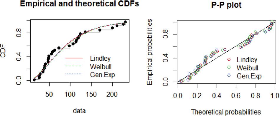
Figure 3 The plot of empirical and theoretical c.d.f’s and P–P plot for data X.

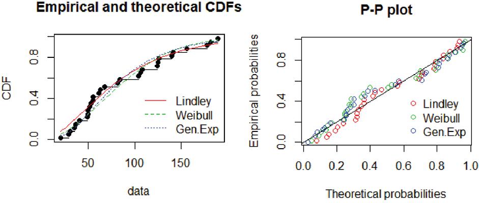
Figure 4 The plot of empirical and theoretical c.d.f’s and P–P plot for data Y.

Further, a Multiplier bootstrap-based goodness–of–fit test introduced by Genest et al. (2013) [18] is performed to assess the relevance of copulas for the real data, the results are reported in Table 5.

Table 5 Goodness of fit test for FGM copula

	Statistic	$\widehat{\tau }$	P-value
Anderson-Darling-type($R_n$)	0.29031	0.46704	0.3981

Table 6 The estimates of the parameters of FGM distributions

Model	${\widehat{\theta }}_1$	${\widehat{\alpha }}_1$	${\widehat{\theta }}_2$	${\widehat{\alpha }}_2$	$\widehat{\tau }$	AIC	BIC
FGM-Lindley	0.0232	4.3305	0.0227	2.3709	0.4416	646.3275	653.3335
FGM-Weibull	0.2134	1.4521	0.2168	2.4681	0.4194	864.1584	871.1643
FGM-Gen.Exp	0.4065	0.0056	0.5794	0.0088	0.4528	685.3983	692.4043

Finally, the bivariate Lindley distribution based on FGM copula are fitted to the data set. A comparison study is performed between FGMBL distribution, FGMBW (El-Sherpieny et al. (2018) [17]), and FGMBGE (Turk et al. (2017) [52]) distributions based on Akaike’s Information Criteria (AIC) and Bayesian Information Criteria (BIC) ( kuha (2004)) [30]). The results are presented in Table 6.

Table 7 The estimates, the corresponding standard deviation of the parameters and reliability parameter of FGMBL distribution

Method	Estimate	${\widehat{\theta }}_1$	${\widehat{\alpha }}_1$	${\widehat{\theta }}_2$	${\widehat{\alpha }}_2$	$\widehat{\tau }$	$\widehat{R}$
MLE	Mean	0.0232	4.3305	0.0226	2.3709	0.4416	0.9812
	(SD)	(0.0029)	( 0.4217)	(0.0004)	(0.0155)	(0.5794)
IFM	Mean	0.0222	0.5681	0.0125	0.0256	2.2331	0.9996
	(SD)	(0.0027)	(0.0186)	(0.0290)	(0.1766)	(0.5683)
SP	Mean	–	–	–	–	0.4964	–
	(SD)					(0.5232)

10 Concluding Remarks

In this article, we studied the estimation of dependent stress-strength reliability R based on FGM copula for Lindley marginals. The FGMBL distribution is proposed and its several statistical properties are derived in a closed-form. Further, the condition for the FGMBL distribution satisfies the positive (negative) quadrant dependence property, and the IFR (DFR) distribution for positive (negative) values of the dependence parameter are also derived.

We estimated the expression of R, by using MLE and IFM methods and investigated its variation with respect to the dependence parameter $\tau$. From the simulation results, we found that the estimated values of R and $\tau$ are closer to the true value in all the considered methods. Further, the MLE method performs better as compared to the other methods for estimating both the dependence parameter $\tau$ and R in terms of MSE. Furthermore, we observe that the variation of the estimate of R with respect to the variation of the dependence parameter $\tau$ is positive, i.e., the variation in R decreases (increases) while $\tau$ decreases (increases). The length of the asymptotic confidence interval and their associated coverage probability of the estimate of the dependence parameter $\tau$ are also obtained.

Finally, a real data set is considered to demonstrate the application of the proposed model, and it shows that the FGMBL distribution is the best choice as compared to FGMBW and FGMBGE distributions based on AIC and BIC. Therefore, the proposed FGM based bivariate Lindley is best choice for dependence stress-strength modelling. As for future research perspectives, asymptotic properties of FGMBL distribution may consider in further. Moreover, different families of stress and strength distributions as well as other families of copulas can be analyzed and the corresponding value of R and their associated properties can be derived.

Acknowledgment

We would like to thank the Editor-In-Chief and anonymous reviewers for a careful reading of the manuscript and several useful suggestions that helped to improve the quality of the paper.

References

[1] Ahmed, D., Sohair, K., and Mokhli, N. (2020). Inference for stress-strength models based on the bivariate general farlie-gumbel-morgenstern distributions. Journal of Statistics Applications & Probability Letters, 7(3):141–150.

[2] Al-Mutairi, D. K., Ghitany, M. E., and Kundu, D. (2013). Inferences on stress-strength reliability from lindley distributions. Communications in Statistics - Theory and Methods, 42:1443 – 1463.

[3] Altun, E. and Cordeiro, G. M. (2020). The unit-improved second-degree lindley distribution: inference and regression modeling. Computational Statistics, 35(1):259–279.

[4] Bai, X., Li, X., Balakrishnan, N., and He, M. (2021). Statistical inference for dependent stress–strength reliability of multi-state system using generalized survival signature. Journal of Computational and Applied Mathematics, 390:113316.

[5] Bakouch, H. S., Al-Zahrani, B. M., Al-Shomrani, A. A., Marchi, V. A. A., and Louzada, F. (2012). An extended lindley distribution. Journal of the Korean Statistical Society, 41(1):75–85.

[6] Barbiero, A. (2017). Assessing how the dependence structure affects the reliability parameter of the strength-stress model. In UNCECOMP, pages 640–650. Institute of Structural Analysis and Antiseismic Research School of Civil.

[7] Baro-Tijerina, M., Piña-Monárrez, M. R., and Villa-Covarrubias, B. (2020). Stress-strength weibull analysis with different shape parameter $\beta$ and probabilistic safety factor. Dyna, 87(215):28–33.

[8] Barreto-Souza, W. and Bakouch, H. S. (2013). A new lifetime model with decreasing failure rate. Statistics, 47(2):465–476.

[9] Basu, A. (1971). Bivariate failure rate. Journal of the American Statistical Association, 66(333):103–104.

[10] Birnbaum, Z. W. and McCarty, R. C. (1958). A distribution$-$free upper confidence bound for pr(Y$<$X)  based on independent samples of x and y. The Annals of Mathematical Statistics, 29(2):558–562.

[11] Biswas, A., Chakraborty, S., and Mukherjee, M. (2021). On estimation of stress–strength reliability with log-lindley distribution. Journal of Statistical Computation and Simulation, 91(1):128–150.

[12] Chandra, N. and Pandey, M. (2012). Bayesian reliability estimation of bivariate marshal-olkin exponential stress-strength model. International Journal of Reliability and Applications, 13(1):37–47.

[13] Chandra, N. and Rathaur, V. K. (2020). Inferences on non-identical stress and generalized augmented strength reliability parameters under informative priors. International Journal of Reliability, Quality and Safety Engineering, 27(04):2050014.

[14] Clayton, D. G. (1978). A model for association in bivariate life tables and its application in epidemiological studies of familial tendency in chronic disease incidence. Biometrika, 65(1):141–151.

[15] Domma, F. and Giordano, S. (2012). A stress–strength model with dependent variables to measure household financial fragility. Statistical Methods & Applications, 21(3):375–389.

[16] Domma, F. and Giordano, S. (2013). A copula-based approach to account for dependence in stress-strength models. Statistical Papers, 54(3):807–826.

[17] El-Sherpieny, E. A., Muhammed, H. Z., and Almetwally, E. M. (2018). Fgm bivariate weibull distribution. In Proceedings of the Annual Conference in Statistics (${\mathrm{53}}^{r\mathit{}d}$), Computer Science, and Operations Research, Institute of Statistical Studies and Research, Cairo University, pages 55–77. https://www.researchgate.net/publication/332109204_FGM_Bivariate_Weibull_Distribution.

[18] Genest, C., Huang, W., and Dufour, J.-M. (2013). A regularized goodness-of-fit test for copulas. Journal de la Société française de statistique, 154(1):64–77.

[19] Ghitany, M. E., Al-Mutairi, D. K., and Aboukhamseen, S. (2015). Estimation of the reliability of a stress-strength system from power lindley distributions. Communications in Statistics-Simulation and Computation, 44(1):118–136.

[20] Ghitany, M. E., Alqallaf, F., Al-Mutairi, D. K., and Husain, H. A. (2011). A two-parameter weighted lindley distribution and its applications to survival data. Mathematics and Computers in simulation, 81(6):1190–1201.

[21] Ghitany, M. E., Atieh, B., and Nadarajah, S. (2008). Lindley distribution and its application. Mathematics and computers in simulation, 20(1):493–506.

[22] Gupta, P. K. and Singh, B. (2013). Parameter estimation of lindley distribution with hybrid censored data. International Journal of System Assurance Engineering and Management, 4(4):378–385.

[23] Gupta, R. C. and Subramanian, S. (1998). Estimation of reliability in a bivariate normal distribution with equal coefficients of variation. Communications in Statistics-Simulation and Computation, 27(3):675–698.

[24] Harris, R. (1970). A multivariate definition for increasing hazard rate distribution functions. The Annals of Mathematical Statistics, 41(2):713–717.

[25] Joe, H. (2005). Asymptotic efficiency of the two-stage estimation method for copula-based models. Journal of multivariate Analysis, 94(2):401–419.

[26] Johnson, N. L. and Kotz, S. (1975). A vector multivariate hazard rate. Journal of Multivariate Analysis, 5(1):53–66.

[27] Khan, A. H. and Jan, T. R. (2015). Estimation of stress-strength reliability model using finite mixture of two parameter lindley distributions. Journal of Statistics Applications and Probability, 4(1):147–159.

[28] Kim, G., Silvapulle, M. J., and Silvapulle, P. (2007). Comparison of semiparametric and parametric methods for estimating copulas. Computational Statistics & Data Analysis, 51(6):2836–2850.

[29] Kotz, S. and Pensky, M. (2003). The stress-strength model and its generalizations: theory and applications. World Scientific.

[30] Kuha, J. (2004). AIC and BIC: Comparisons of assumptions and performance. Sociological methods & research, 33(2):188–229.

[31] Kundu, D. and Raqab, M. Z. (2015). Estimation of R$=P(Y<X)$ for three-parameter generalized rayleigh distribution. Journal of Statistical Computation and Simulation, 85(4):725–739.

[32] Lehmann, E. L. (1966). Some concepts of dependence. The Annals of Mathematical Statistics, 37(5):1137–1153.

[33] Lindley, D. (1965). Probability and statistics 2. inference.

[34] Lindley, D. V. (1958). Fiducial distributions and bayes’ theorem. Journal of the Royal Statistical Society. Series B (Methodological), 78(4):102–107.

[35] Mazucheli, J. and Achcar, J. A. (2011). The lindley distribution applied to competing risks lifetime data. Computer methods and programs in biomedicine, 104(2):188–192.

[36] McGilchrist, C. A. and Aisbett, C. W. (1991). Regression with frailty in survival analysis. Biometrics, 47f(2):461–466.

[37] Morgenstern, D. (1956). Einfache beispiele zweidimensionaler verteilungen. Mitteilingsblatt fur Mathematische Statistik, 8:234–235.

[38] Mustafa Ç. Korkmaz, Haitham M. Yousof, M. R. and Hamedani, G. G. (2018). The odd lindley burr xii model: Bayesian analysis, classical inference and characterizations. Journal of data science, 16:327–354.

[39] Nelsen, R. B. (2007). An introduction to copulas. Springer Science & Business Media.

[40] Oakes, D. (1989). Bivariate survival models induced by frailties. Journal of the American Statistical Association, 84(406):487–493.

[41] Patil, D. D. and Naik-Nimbalkar, U. V. (2017). Computation and estimation of reliability for some bivariate copulas with pareto marginals. Journal of Statistical Computation and Simulation, 87(18):3563–3589.

[42] Rostamian, S. and Nematollahi, N. (2019). Estimation of stress–strength reliability in the inverse gaussian distribution under progressively type ii censored data. Mathematical Sciences, 13(2):175–191.

[43] Sankaran, P. G. and Nair, N. U. (1991). On bivariate vitality functions. In Proceeding of National Symposium on Distribution Theory.

[44] Sarra, C. and Zeghdoudi, H. (2021). The xlindley distribution: Properties and application. Journal of Statistical Theory and Applications, 20:318–327.

[45] Shaked, M. (1977). A family of concepts of dependence for bivariate distributions. Journal of the American Statistical Association, 72(359):642–650.

[46] Shanbhag, D. N. and Kotz, S. (1987). Some new approaches to multivariate probability distributions. Journal of Multivariate Analysis, 22(2):189–211.

[47] Shanker, R. and Mishra, A. (2013). A quasi lindley distribution. African Journal of Mathematics and Computer Science Research, 6(4):pp–64.

[48] Shanker, R., Sharma, S. N., and Shanker, R. (2013). A two-parameter lindley distribution for modeling waiting and survival times data. Applied Mathematics-a Journal of Chinese Universities Series B, 4:363–368.

[49] Sharma, V. K., Singh, S. K., Singh, U., and Agiwal, V. (2015). The inverse lindley distribution: a stress-strength reliability model with application to head and neck cancer data. Journal of Industrial and Production Engineering, 32(3):162–173.

[50] Singh, S. K., Singh, U., and Sharma, V. K. (2014). Estimation on system reliability in generalized lindley stress-strength model. Journal of Statistics Applications & Probability, 3(1):61.

[51] Sklar, A. (1973). Random variables, joint distribution functions, and copulas. Kybernetika, 9(6):449–460.

[52] Turk, L. I. A., Elaal, M. K. A., and Jarwan, R. S. (2017). Inference of bivariate generalized exponential distribution based on copula functions. Applied Mathematical Sciences, 11(24):1155–1186.

[53] Vaidyanathan, V. S. and Sharon Varghese, A. (2016). Morgenstern type bivariate lindley distribution. Statistics, Optimization & Information Computing, 4(2):132–146.

[54] Xu, J. J. (1996). Statistical modelling and inference for multivariate and longitudinal discrete response data. PhD thesis, University of British Columbia.

Biographies

A. James has received M.Sc. (Statistics) in 2017 from St. Thomas College, Thrissur and pursuing for Ph.D. (Statistics) degree in the Department of Statistics, Ramanujan School of Mathematical Sciences at Pondicherry University, India. Her research interest is Copula based stress-strength modelling in reliability theory.

N. Chandra is an active senior faculty and researcher in the Department of Statistics, Ramanujan School of Mathematical Sciences at Pondicherry University, India. He has received Ph.D. (Statistics) degree in 2002 from Banaras Hindu University, India. Dr. Chandra is a recipient of Senior Research Fellow. He is presently working on competing risk hazards analysis and dependence stress-strength reliability modelling. His research interests include Classical and Bayesian inference, life testing and reliability modelling and Cox’s PH modelling in survival analysis, Accelerated life testing and Augmenting strength reliability.

M. Pandey received her Ph.D. degree in Statistics in 1977 from Banaras Hindu University, Varanasi, India. Her major field of study is Preliminary Test Statistical Inference, Reliability Theory, Bayesian reliability, Stress-strength model in reliability and Biostatistics. She is retired Professor of Biostatistics and presently associated with Department of Science and Technology Centre for Interdisciplinary Mathematical Sciences, Government of India at Institute of Science, Banaras Hindu University, Varanasi, India. Her current research interest are Estimation in Accelerated Life Testing, Bayesian Estimation of Family of Bivariate Exponential Models under Stress – strength setup, Environmental Pollution and Application of Multivariate Techniques.

Journal of Reliability and Statistical Studies, Vol. 15, Issue 1 (2022), 341–380.
doi: 10.13052/jrss0974-8024.15114
© 2022 River Publishers