PCM Transformation: Properties and Their Estimation

Dinesh Kumar, Pawan Kumar^*, Pradip Kumar, Sanjay Kumar Singh and Umesh Singh

Department of Statistics, Banaras Hindu University, Varanasi, India

E-mail: pawanchauhanstranger@gmail.com

${}^{*}$Corresponding Author

Received 21 January 2021; Accepted 06 June 2021; Publication 06 July 2021

Abstract

In the present piece of work, we are going to propose a new trigonometry based transformation called PCM transformation. We have been obtained its various statistical properties such as survival function, hazard rate function, reverse-hazard rate function, moment generating function, median, stochastic ordering etc. Maximum Likelihood Estimator (MLE) method under classical approach and Bayesian approaches are tackled to obtain the estimate of unknown parameter. A real dataset has been applied to check its fitness on the basis of fitting criterions Akaike Information criterion (AIC), Bayesian Information criterion (BIC), log-likelihood (-LL) and Kolmogrov-Smirnov (KS) test statistic values in real sense. A simulation study is also being conducted to assess the estimator’s long-term attitude and compared over some chosen distributions.

Keywords: Maximum likelihood estimator, moment generating function, $PC{M}_E(\theta )$-distribution, absolute relative bias (ARB), simulation study.

1 Introduction

From many years ago, we are seeing a race is continued for establishing, proposing and generalizing distributions and researchers are showing their keen interest to propose new distribution which are more flexible, applicable in real life scenario, till now this become a major challenge for us. So, to beat such challenges young researchers are proposing a series of new distributions day-by-day and checking their superiority, flexibility and applicability to real life problems. Hazard rate is quite useful tool for identifying the nature of chosen lifetime models and projects various patterns like- increasing failure rate (IFR), decreasing failure rate (DFR), upside-down bathtub (UBT) and bath-tub shape (BT) and for elaborative study readers may refer Glaser (1980). Exponential distribution plays very constructive role in studying the lifetime phenomena but use of distribution is quite restrictive due to its constant hazard rate nature. So, to overcome it, Weibull distribution and gamma distribution are widely used and usually preferred. Weibull distribution also plays a key role in non-constant hazard rate model, for this pertinence Mudholkar and Srivastava (1993), Xie and Lai (1996), and Xie et al. (2002) introduced three parameter generalization of Weibull distribution for analyzing bathtub shaped failure rate pattern. Lifetime distributions are the basis for analyzing and judging the real life problems. There are many researchers which have proposed many new distributions those are suitable for the study in various fields like Medical, Biology, Demography, Insurance, Engineering, Finance, Economics etc. There is no any model to be globally acceptable model, to deal such situations, there is need to develop new model(s)/distribution(s). Datasets are also important for checking the suitability and flexibility of the considered model. Here, we have used complete datasets only. Recent studies are demonstrating great interest in the continuous distributions, few of them are circular Cauchy distribution given by Kent and Tyler (1988), Abate et al. (1995) proposed the weighted-cosine exponential distribution, Nadarajah and Kotz (2006) proposed the beta-type distribution, Al-Faris and Khan (2008) proposed the sine square distribution and Sinha (2012) proposed the Sinoform distribution. As we all know that there is a shortfall of trigonometric transformations and plethora of other than trigonometric type transformations in the statistical literature. Therefore, we are keen interested to propose a new trigonometric transformation and also check its flexibility.

In Statistical literature no. of transformations are available to produce new CDF corresponding to a given CDF. Suppose, we have a CDF $F(x)$, then the associated proposed CDF will be $G_i(x)$.

• The most popular among them is the power transformation initiated by Gupta et al. (1998) having the form

$$G_1(x)=[{(F(x)]}^{\alpha };\alpha >0$$

• Quadratic rank transformation map (QRTM) proposed by Shaw and Buckley (2009) having the form

$$G_2(x)=(1+\lambda )F(x)-\lambda F^2(x);|\lambda |\le 1$$

• DUS transformation proposed by Kumar et al. (2015) having the form

$$G_3(x)=\left(\frac{e^{F(x)}-1}{e-1}\right);e=\exp (1)$$

• SS-transformation proposed by Kumar et al. (2015) having the form

$$G_4(x)=\sin \left(\frac{\pi }{2}F(x)\right)$$

• Minimum Guarantee (MG)-distribution proposed by Kumar et al. (2017) having the form

$$G_5(x)=e^{1-\frac{1}{F(x)}}$$

• log-transformation proposed by Maurya et al. (2016) and having the form

$$G_6(x)=1-\frac{\ln (2-F(x))}{\ln 2}$$

• Transformation based on the generalization of Kumar et al. (2015) called GDUS transformation proposed by Maurya et al. (2017) having the form

$$G_7(x)=\left(\frac{e^{F^{\alpha }(x)}-1}{e-1}\right);\alpha >0$$

• New Sine-G family based on Kumar et al. (2015) proposed by Mahmood and Chesneau (2019) with its nice form

$$G_8(x)=\sin \left(\frac{\pi }{4}F(x)\left(F(x)+1\right)\right)\mathit{\hspace{1em}}\forall x\in \mathrm{\Re }$$

• New transformation initiated by Kyurkchiev (2017) to develop a sigmoid family of functions for Verhulst Logistic function is

$$G_9(x)=\frac{2F(x)}{1+F(x)}$$

• Cosine-Sine (CS) transformation proposed by Chesneau et al. (2018) and its nice form is

$$G_{10}(x)=\frac{(\alpha +\gamma )\sin \left(\frac{\pi }{2}F(x)\right)}{\begin{array}{c}\alpha +\beta \cos \left(\frac{\pi }{2}F(x)\right)+\gamma \sin \left(\frac{\pi }{2}F(x)\right)\hfill \\ +\theta \sin \left(\frac{\pi }{2}F(x)\right)\cos \left(\frac{\pi }{2}F(x)\right)\hfill \end{array}};\forall x\in \mathrm{\Re }$$

Where $\alpha \ge 0,\beta \ge 0,\gamma \ge 0,\theta \ge 0$ are parameters with $\alpha +\beta >0$, $\alpha +\gamma >0$.

In this continuation, after taking ideas and motivations from the above discussed transformations, we have decided to propose a new transformation commonly known as PCM transformation given below

$$G(x)=\tan \left(\frac{\pi }{4}F(x)\right)$$

(1)

Where, $G(x)$ and $F(x)$ are the CDFs of the proposed transformation and baseline distribution. By definition, we get (1) is the CDF because it satisfies the following properties-

(i) $G(-\mathrm{\infty })=0,G(\mathrm{\infty })=1$

(ii) $G(x)$is monotonic increasing function of $x$.

(iii) $G(x)$is right continuous.

(iv) $0\le G(x)\le 1$

On differentiating (1) w.r.t. $x$, we get the PDF $g(x)$ and is given by

$$g(x)=\frac{\pi }{4}f(x){\sec }^2\left(\frac{\pi }{4}F(x)\right);x>0$$

(2)

To illustrate the usefulness of this new transformation (1), we are considering exponential distribution with mean $\frac{1}{\theta }$ as a baseline distribution. The CDF $G(x)$ and corresponding PDF $g(x)$ of the new lifetime distribution using PCM transformation, viz. (1) and (2) are obtained as follows

$G(x)$	$=\tan \left({\displaystyle \frac{\pi }{4}}\left(1-e^{-\theta x}\right)\right)$
$\Rightarrow G(x)$	$={\displaystyle \frac{1-\tan \left(\frac{\pi }{4}{e}^{-\theta x}\right)}{1+\tan \left(\frac{\pi }{4}{e}^{-\theta x}\right)}}\mathit{\hspace{1em}}\forall x>0,\theta >0$	(3)

and

$g(x)={\displaystyle \frac{\pi }{4}}\theta e^{-\theta x}{\sec }^2\left({\displaystyle \frac{\pi }{4}}\left(1-e^{-\theta x}\right)\right)\mathit{\hspace{1em}}\forall x>0,\theta >0$

(4)

The novelty of the article is that the proposed transformation is parsimonious in parameter. Also, this gives a single parameter distribution having increasing, decreasing and bath-tub shape hazard rate nature for different choices of parameter which seems rarely in some distributions only.

The rest of the article is arranged as follows, statistical measures has been discussed in Section 2, estimation of parameter has been carried out in Section 3, real data application has been shown in Section 4, simulation study have been discussed in Section 5 and concluding remarks has been elaborated in Section 6.

2 Statistical Measures

In this section, we are interested in obtaining the expressions for survival function, hazard rate function, reverse-hazard rate function, moment generating function (MGF), quantile function, sample generation, median, stochastic ordering of $PC{M}_E(\theta )$-distribution.

2.1 Survival Function

The survival function is the likelihood of any lifetime entity living past a certain age $x$ and is denoted by $S(x)$ and defined as

$S(x)=1-{\displaystyle \frac{1-\tan \left(\frac{\pi }{4}{e}^{-\theta x}\right)}{1+\tan \left(\frac{\pi }{4}{e}^{-\theta x}\right)}}={\displaystyle \frac{2\tan \left(\frac{\pi }{4}{e}^{-\theta x}\right)}{1+\tan \left(\frac{\pi }{4}{e}^{-\theta x}\right)}}$

(5)

Figure 1 PDF and Survival plots of $PC{M}_E(\theta )$-distribution for different choices of $\theta$.

2.2 Hazard Rate Function

This is the instantaneous failure rate or force of mortality and is the rate at which any life testing item will stop to work and is denoted by $h(x)$ and defined as the ratio of the PDF to the survival function and is

$$h(x)=\frac{\pi }{8}\left(\frac{\theta e^{-\theta x}{\sec }^2\left(\frac{\pi }{4}\left(1-e^{-\theta x}\right)\right)\left(1+\tan \left(\frac{\pi }{4}{e}^{-\theta x}\right)\right)}{\tan \left(\frac{\pi }{4}{e}^{-\theta x}\right)}\right)$$

(6)

And the respective hazard rate plots for different choices of parameter $\theta$ are shown in Figure 2.

Figure 2 Plots of hazard rate function of $PC{M}_E(\theta )$-distribution for different choices of $\theta$.

2.3 Reverse-Hazard Rate Function

The reverse-hazard rate function, which is defined as the ratio of PDF to CDF, is another measure that can be used in place of the hazard rate function

$$r(x)=\frac{\pi }{4}\left(\frac{\theta e^{-\theta x}{\sec }^2\left(\frac{\pi }{4}\left(1-e^{-\theta x}\right)\right)\left(1+\tan \left(\frac{\pi }{4}{e}^{-\theta x}\right)\right)}{1-\tan \left(\frac{\pi }{4}{e}^{-\theta x}\right)}\right)$$

(7)

2.4 Quantiles

The $p^{th}$ quantile of $PC{M}_E(\theta )$-distribution can be obtained by the solution of the equation

$G(x_p)$	$=p$
$\Rightarrow x_p$	$=-{\displaystyle \frac{1}{\theta }}\ln \left(1-{\displaystyle \frac{4}{\pi }}{\tan }^{-1}p\right)$	(8)

2.5 Median

Median is the most basic measure of central tendencies; it’s the quantity that divides total likelihood into two equal portions that can be obtained by the relation $G(M)=0.5\Rightarrow M=G^{-1}(0.5)$. Thus, on putting $p=0.5$ in (8), we get the required expression for median of $PC{M}_E(\theta )$-distribution as follows

$$M=-\frac{1}{\theta }\ln \left(1-\frac{4}{\pi }{\tan }^{-1}0.5\right)$$

(9)

2.6 Sample Generation

The simple and most popular method to generate a sample is the inverse CDF transformation method. If $X$ is $U(0,1)$ with CDF $F(x)$, then by the transformation, we generate the sample from the equation $G(x)=U\Rightarrow x=G^{-1}(U)$ of $PC{M}_E(\theta )$-distribution

$$x=-\frac{1}{\theta }\ln \left(1-\frac{4}{\pi }{\tan }^{-1}U\right)$$

(10)

2.7 Stochastic Ordering

Let us take the random variables $X_1$ and $X_2$ having CDFs $G_1(x)$ and $G_2(x)$ with parameters ${\theta }_1$ and ${\theta }_2$ respectively, then by definition, we can say that the variable $X_1$ is stochastically greater than $X_2$, if $G_1(x)\le G_2(x)$ (See Gupta et al. (1998)).

Now, if random variables $X_1$ and $X_2$ following $PC{M}_E(\theta )$-distribution, then for ${\theta }_1<{\theta }_2$

${\displaystyle \frac{G_1(x)}{G_2(x)}}$	$={\displaystyle \frac{\left(1+\tan \left(\frac{\pi }{4}{e}^{-{\theta }_{2}x}\right)\right)\left(1-\tan \left(\frac{\pi }{4}{e}^{-{\theta }_{1}x}\right)\right)}{\left(1+\tan \left(\frac{\pi }{4}{e}^{-{\theta }_{1}x}\right)\right)\left(1-\tan \left(\frac{\pi }{4}{e}^{-{\theta }_{2}x}\right)\right)}}\le 1$
$\Rightarrow G_1(x)$	$\le G_2(x)\mathit{\hspace{1em}}\forall x$

So, we say that $X_1$ is stochastically greater than $X_2$ for ${\theta }_1<{\theta }_2$.

2.8 Moment Generating Function

The Moment Generating Function (MGF) of r.v. $X$ is denoted by $M_X(t)$, if it exists for every $t$ in some interval containing zero i.e. $t\in (-h,h)$ and defined as

$M_X(t)$	$={\displaystyle {\int }_0^{\mathrm{\infty }}}{e}^{tx}g(x)\mathit{d}x$
	$={\displaystyle {\int }_0^{\mathrm{\infty }}}{e}^{tx}\times {\displaystyle \frac{\pi }{4}}\theta e^{-\theta x}{\sec }^2\left({\displaystyle \frac{\pi }{4}}\left(1-e^{-\theta x}\right)\right)\mathit{d}x$
	$={\displaystyle {\int }_0^{\pi /4}}\underset{w(x)}{\overset{t/\theta }{\underbrace{\left({\displaystyle \frac{\pi }{\pi -4k}}\right)}}}\underset{\varphi (x)}{\underbrace{{\sec }^{2}k}}dk\mathit{\hspace{1em}}[\because {\displaystyle \frac{\pi }{4}}(1-e^{-\theta x})=k]$

Now, for checking the convergence of the integral, we follow the test as mentioned below,

Abel’s Test

If ${\int }_a^{b}w(x)\mathit{d}x$ is convergent and $\varphi (x)$ is bounded and monotonic in $(a,b)$, then ${\int }_a^{b}w(x)\varphi (x)\mathit{d}x$ also convergent.

It is obvious that ${\sec }^{2}k$ is monotonically increasing function and bounded in $(0,\pi /4)$.

Now, our aim is to check the convergence of ${\int }_0^{\pi /4}{\left(\frac{\pi }{\pi -4k}\right)}^{t/\theta }\mathit{d}k$.

So,

${\displaystyle {\int }_0^{\pi /4}}{\left({\displaystyle \frac{\pi }{\pi -4k}}\right)}^{t/\theta }\mathit{d}k$

$\mathrm{\hspace{1em}\hspace{1em}}={\displaystyle \frac{\pi }{2}}{\displaystyle {\int }_0^{\pi /2}}{\sin }^{1-2t/\theta }p\times \cos pdp\mathit{\hspace{1em}}[\because 4k=\pi {\cos }^{2}p]$

$\mathrm{\hspace{1em}\hspace{1em}}={\displaystyle \frac{\pi }{4}}{\displaystyle \frac{\mathrm{\Gamma }\left(1-\frac{t}{\theta }\right)\mathrm{\Gamma }(1)}{\mathrm{\Gamma }\left(2-\frac{t}{\theta }\right)}}\mathit{\hspace{1em}}\forall t<\theta$

$\mathrm{\hspace{1em}\hspace{1em}}\mathit{\hspace{1em}}[\because {\displaystyle {\int }_0^{\pi /2}}{\sin }^m(p)\times {\cos }^n(p)dp={\displaystyle \frac{\mathrm{\Gamma }\left(\frac{m+1}{2}\right)\mathrm{\Gamma }\left(\frac{n+1}{2}\right)}{2\mathrm{\Gamma }\left(\frac{m+n+2}{2}\right)}}]$

Hence, by Abel’s test ${\int }_0^{\pi /4}{\left(\frac{\pi }{\pi -4k}\right)}^{t/\theta }{\sec }^{2}kdk$ converges $\forall t<\theta$. This shows that MGF exists $\forall t<\theta$.

3 Estimation of Parameter

In this section, we are going to obtain the estimate of unknown parameter $\theta$ involved in the $PC{M}_E(\theta )$-distribution by considering the classical as well as Bayesian Paradigm.

3.1 Maximum Likelihood Estimator

This is the most popular and extensively used method initiated by C.F. Gauss and elaborative study initiated by Prof. R. A. Fisher to obtain the estimator of the unknown parameter of the distribution. If $X_1,X_2,\mathrm{\dots },X_n$ be a set of random observations from the population $PC{M}_E(\theta )$-distribution having PDF $g(x;\theta )$, then its likelihood function will be as follows

$L={\displaystyle \prod _{i=1}^n}{\displaystyle \frac{\pi }{4}}\theta e^{-\theta x_i}{\sec }^2\left({\displaystyle \frac{\pi }{4}}\left(1-e^{-\theta x_i}\right)\right)$

Taking natural logarithm on both sides, we get

$$S=\ln (L)=C+n\ln (\theta )-\theta \sum _{i=1}^n{x}_i+2\sum _{i=1}^n\ln \left(\sec \left(\frac{\pi }{4}\left(1-e^{-\theta x_i}\right)\right)\right);$$
$$C={\left(\frac{\pi }{4}\right)}^n$$	(11)

On differentiating (11) with respect to the parameter $\theta$ and equating the resultant to $0$, we have

${\displaystyle \frac{dS}{d\theta }}={\displaystyle \frac{n}{\theta }}-{\displaystyle \sum _{i=1}^n}{x}_i+{\displaystyle \frac{\pi \theta }{2}}{\displaystyle \sum _{i=1}^n}{e}^{-\theta x_i}\tan \left({\displaystyle \frac{\pi }{4}}\left(1-e^{-\theta x_i}\right)\right)=0$

(12)

Above Equation (12) is not solvable analytically. So, we impose $nlm()$ function by using $R$ software to solve it numerically to obtain the estimate ${\widehat{\theta }}_M$ of $\theta$.

3.2 Bayes Estimator

Another branch of drawing inferences about the population parameters is the Bayesian Paradigm. Under this setup the unknown parameter(s) is/are not taken as constant but will be a random variable and having a distribution called prior distribution. With the help of prior distribution our next step is to obtain the posterior distribution which can easily be obtained after the prior information. The important part of Bayesian paradigm is to choose an appropriate loss function, which is not an easy job. Some important loss functions are squared error loss function (SELF), General entropy loss function (GELF) and LINEX loss function are usually preferred. For the extensive study about the suitable loss function and Bayesian estimation readers may refer to Singh (2011), Singh et al. (2011), Singh et al. (2013), Kumar et al. (2019), Ali et al. (2019), Yousaf et al. (2020), Shajid et al. (2020), Ali et al. (2020), Mansoor et al. (2020) and Dey et al. (2020). For the study, we are choosing the $\gamma (a,b)$-distribution as a prior information having PDF of the form

$$\tau (\theta )=\frac{a^b{e}^{-a\theta }{\theta }^{b-1}}{\mathrm{\Gamma }b}$$

(13)

Here, $a>0,b>0$ are the hyper-parameters and can be obtained when prior mean and prior variance will be known. These hyper-parameters can be obtained, if we have two independent informations available on $\theta$, information can be obtained from prior mean and prior variance readers may see Singh (2011). For (13) prior mean and variance are $M=\frac{b}{a}$ and $V=\frac{b}{a^2}$, respectively and gives $a=\frac{M}{V}$ and $b=\frac{M^2}{V}$. Also, (13) will behave like non-informative prior for any finite value of $M$ and $V$ be sufficiently large.

The PDF of posterior distribution corresponding to the prior distribution $\gamma (a,b)$, viz. $\varphi (\theta |\underset{¯}{X})$ for a given sample $\underset{¯}{X}=(x_1,x_2,\mathrm{\dots },x_n)$ is obtained as follows

$\varphi \left(\theta |\underset{¯}{X}\right)={\displaystyle \frac{{\theta }^{n+b-1}{e}^{-\theta \left(a+{\sum }_{i=1}^n{x}_i\right)}{\prod }_{i=1}^n{\sec }^2\left(\frac{\pi }{4}\left(1-e^{-\theta x_i}\right)\right)}{{\int }_0^{\mathrm{\infty }}{\theta }^{n+b-1}{e}^{-\theta \left(a+{\sum }_{i=1}^n{x}_i\right)}{\prod }_{i=1}^n{\sec }^2\left(\frac{\pi }{4}\left(1-e^{-\theta x_i}\right)\right)d\theta }}$ (14)

Here we observed that, (14) cannot be solved analytically and hence Bayes estimators under considered loss function cannot be solved analytically. Therefore, we propose to use some numerical approximation technique to solve them approximately.

Now, we will consider squared error loss function (SELF) and general entropy loss function (GELF) to obtain Bayes estimator of $\theta$, which are defined as

$L_S({\widehat{\theta }}_S,\theta )$	$={({\widehat{\theta }}_S-\theta )}^2$	(15)
$L_G({\widehat{\theta }}_G,\theta )$	$={\left({\displaystyle \frac{{\widehat{\theta }}_G}{\theta }}\right)}^{\delta }-\delta \ln \left({\displaystyle \frac{{\widehat{\theta }}_G}{\theta }}\right)-1$	(16)

and the corresponding Bayes estimators are

${\widehat{\theta }}_S=E(\theta |\underset{¯}{X})=\left[{\displaystyle \frac{{\int }_0^{\mathrm{\infty }}{\theta }^{n+b}{e}^{-\theta \left(a+{\sum }_{i=1}^n{x}_i\right)}{\prod }_{i=1}^n{\sec }^2\left(\frac{\pi }{4}\left(1-e^{-\theta x_i}\right)\right)d\theta }{{\int }_0^{\mathrm{\infty }}{\theta }^{n+b}{e}^{-\theta \left(a+{\sum }_{i=1}^n{x}_i\right)}{\prod }_{i=1}^n{\sec }^2\left(\frac{\pi }{4}\left(1-e^{-\theta x_i}\right)\right)d\theta }}\right]$

and

${\widehat{\theta }}_G$	$=E{\left({\theta }^{-\delta }|\underset{¯}{X}\right)}^{\frac{-1}{\delta }}$
	$={\left[{\displaystyle \frac{{\int }_0^{\mathrm{\infty }}{\theta }^{n+b-\delta -1}{e}^{-\theta \left(a+{\sum }_{i=1}^n{x}_i\right)}{\prod }_{i=1}^n{\sec }^2\left(\frac{\pi }{4}\left(1-e^{-\theta x_i}\right)\right)d\theta }{{\int }_0^{\mathrm{\infty }}{\theta }^{n+b-\delta -1}{e}^{-\theta \left(a+{\sum }_{i=1}^n{x}_i\right)}{\prod }_{i=1}^n{\sec }^2\left(\frac{\pi }{4}\left(1-e^{-\theta x_i}\right)\right)d\theta }}\right]}^{\frac{-1}{\delta }}$	(18)

respectively.

Here, $\delta$ is the loss parameter of GELF and for $\delta =-1$, the Bayes estimator under GELF (18) reduces to Bayes estimator under SELF (17). Also, the Equations (17) and (18) are not in nice closed form so to solve them by using Gauss-Laguerre quadrature technique through R software to obtain the solution approximately.

4 Real Data Illustration

To demonstrate real dataset application of the proposed $PC{M}_E(\theta )$-distribution, we have considered the data set of remission times of 128 bladder cancer patients. For assessing superiority of $PC{M}_E(\theta )$-distribution on this data set, we consider Transmuted Inverse Weibull distribution (TIWD), Inverse Weibull distribution (IWD), Transmuted Inverse exponential distribution (TIED) and Transmuted Inverse Rayleigh distribution (TIRD) as rival distributions. The fitting criterions used here are Akaike Information criterion (AIC), Bayesian Information criterion (BIC), -log likelihood (-LL) and Kolmogorov-Smirnov (KS)-test statistic. The MLE of parameter $\theta$ of $PC{M}_E(\theta )$-distribution based on this data set is obtained as 0.1279712 and consequently the values of criterions are calculated and shown in Table 1. The values of the criterions for other considered distributions have been extracted from Khan and Khan (2014) and are also shown in comparative Table 1.

From comparative Table 1, it is clear that the values of AIC, BIC, -LL and KS-test statistics of $PC{M}_E(\theta )$-distribution is least as compared to other considered distributions. So, we can say that our proposed distribution outperforms the other considered distributions TIWD, IWD, TIED and TIRD.

Table 1 AIC, BIC, -LL and KS test values of data of remission times for the chosen distributions

Distributions	AIC	BIC	-LL	KS
$PC{M}_E(\theta )$	835.600	838.400	415.300	0.076
TIWD	879.400	879.700	438.500	0.119
IWD	892.000	892.200	444.000	0.131
TIED	889.600	889.800	442.800	0.155
TIRD	1424.400	1424.600	710.200	0.676

The plot of empirical CDF $F_n(x)$ and fitted CDF $G(x)$ of $PC{M}_E(\theta )$-distribution against the remission times (in months) of 128 bladder cancer patients data extracted from Lee and Wang (2003) and shown in Figure 3.

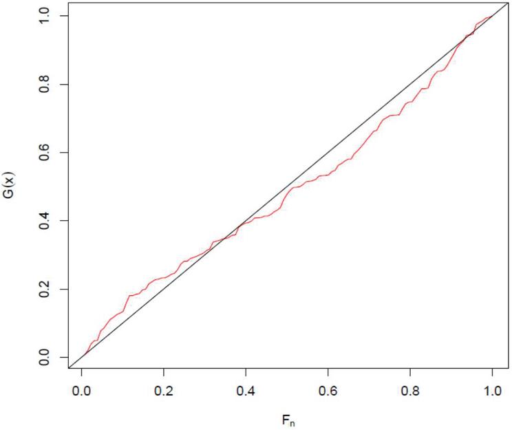
Figure 3 Plot of ECDF and fitted CDF of $PC{M}_E(\theta )$-distribution.

5 Simulation Study

In this section, we are trying to know the performance of the estimators for their long-run use. We have obtained simulated risks under SELF and absolute relative bias (ARB) of ${\widehat{\theta }}_M$, ${\widehat{\theta }}_S$ and ${\widehat{\theta }}_G$ on the basis of 5000 simulated samples of different sample sizes. The simulated risks under SELF will be the function of $n,\theta ,\delta ,a$ and $b$. We have arbitrarily chosen the values $\theta =0.5,1.0,1.5$; $\delta =\pm 2$; $a=4,b=8$ and $n=10,15,20,25,30,40,60$. The results are summarized in Tables 2–4. From all three tables, we see that as sample size increases, the values of simulated risks and absolute relative bias (ARBs) decreases.

Table 2 Simulated risks under SELF and Absolute Relative Bias (ARB) of ${\widehat{\theta }}_M$, ${\widehat{\theta }}_S$ and ${\widehat{\theta }}_G$ for the true value of parameter $\theta =0.5$

	Risk				ARB
			${\widehat{\theta }}_G$				${\widehat{\theta }}_G$
n	${\widehat{\theta }}_M$	${\widehat{\theta }}_S$	$\delta =-2$	$\delta =2$	${\widehat{\theta }}_M$	${\widehat{\theta }}_S$	$\delta =-2$	$\delta =2$
10	0.0321	0.1053	0.1171	0.0737	0.2611	0.5260	0.5609	0.4233
15	0.0181	0.0543	0.0599	0.0392	0.1957	0.3759	0.3991	0.3089
20	0.0147	0.0386	0.0422	0.0290	0.1763	0.3132	0.3305	0.2631
25	0.0099	0.0232	0.0252	0.0177	0.1531	0.2352	0.2479	0.2009
30	0.0087	0.0191	0.0207	0.0150	0.1456	0.2166	0.2269	0.1883
40	0.0062	0.0119	0.0128	0.0096	0.1211	0.1676	0.1750	0.1477
60	0.0039	0.0065	0.0069	0.0055	0.0971	0.1258	0.1301	0.1141

Table 3 Simulated risks under SELF and Absolute Relative Bias (ARB) of ${\widehat{\theta }}_M$, ${\widehat{\theta }}_S$ and ${\widehat{\theta }}_G$ for the true value of parameter $\theta =1.0$

	Risk				ARB
			${\widehat{\theta }}_G$				${\widehat{\theta }}_G$
n	${\widehat{\theta }}_M$	${\widehat{\theta }}_S$	$\delta =-2$	$\delta =2$	${\widehat{\theta }}_M$	${\widehat{\theta }}_S$	$\delta =-2$	$\delta =2$
10	0.1333	0.1788	0.2038	0.1154	0.2408	0.3288	0.3557	0.2553
15	0.0864	0.1242	0.1387	0.0869	0.2178	0.2773	0.2954	0.2271
20	0.0543	0.0765	0.0846	0.0562	0.1777	0.2114	0.2237	0.1793
25	0.0446	0.0620	0.0679	0.0472	0.1598	0.1895	0.1993	0.1640
30	0.0361	0.0501	0.0544	0.0390	0.1442	0.1715	0.1797	0.1494
40	0.0224	0.0303	0.0326	0.0244	0.1186	0.1349	0.1403	0.1213
60	0.0158	0.0197	0.0208	0.0168	0.0966	0.1073	0.1106	0.0989

Table 4 Simulated risks under SELF and Absolute Relative Bias (ARB) of ${\widehat{\theta }}_M$, ${\widehat{\theta }}_S$ and ${\widehat{\theta }}_G$ for the true value of parameter $\theta =1.5$

	Risk				ARB
			${\widehat{\theta }}_G$				${\widehat{\theta }}_G$
n	${\widehat{\theta }}_M$	${\widehat{\theta }}_S$	$\delta =-2$	$\delta =2$	${\widehat{\theta }}_M$	${\widehat{\theta }}_S$	$\delta =-2$	$\delta =2$
10	0.2909	0.1619	0.1889	0.1028	0.2640	0.2082	0.2255	0.1686
15	0.1828	0.1281	0.1447	0.0907	0.2119	0.1815	0.1932	0.1553
20	0.1249	0.0989	0.1099	0.0738	0.1714	0.1574	0.1665	0.1359
25	0.0839	0.0732	0.0804	0.0589	0.1475	0.1383	0.1452	0.1230
30	0.0804	0.0719	0.0780	0.0576	0.1433	0.1357	0.1413	0.1226
40	0.0532	0.0494	0.0526	0.0420	0.1179	0.1138	0.1176	0.1053
60	0.0352	0.0332	0.0346	0.0300	0.0963	0.0923	0.0941	0.0890

On the basis of Tables 3 and 4, we found that ${\widehat{\theta }}_M$ performs better as compared to ${\widehat{\theta }}_S$ and ${\widehat{\theta }}_G$ in the sense of having smallest risks under SELF and ARB for the true values of parameter $\theta =0.5,1.0$ while from Table 4, it is clear that, ${\widehat{\theta }}_G(\delta =2)$ performs better as compared to ${\widehat{\theta }}_M$ and ${\widehat{\theta }}_S$ in the sense of having smallest values of simulated risks under SELF and ARB both for $\theta =1.5$.

6 Concluding Remarks

In this piece of work, we have proposed PCM-transformation in order to get a parsimonious transformed lifetime distribution of some available baseline lifetime distribution. PCM-transformation of $\exp (\theta )$-distribution has been considered to check its application to the real problem. Several estimators such as MLE, Bayes estimators under SELF and GELF of the parameter $\theta$ of $PC{M}_E(\theta )$-distribution has been obtained. A real dataset of remission times of 128 bladder cancer patients has been considered and it was found better fit by $PC{M}_E(\theta )$-distribution as compared to TIWD, IWD, TIED and TIRD in terms of smallest values of AIC, BIC, -LL and KS-test statistics. Simulation study has also been carried out to know the performances of ${\widehat{\theta }}_M$, ${\widehat{\theta }}_S$ and ${\widehat{\theta }}_G$ for their long-run use and it has been found that for $\theta =0.5,1.0$, ${\widehat{\theta }}_M$ performs better as compared to ${\widehat{\theta }}_S$ and ${\widehat{\theta }}_G$, while for $\theta =1.5$, ${\widehat{\theta }}_G(\delta =2)$ performs better as compared to ${\widehat{\theta }}_M$ and ${\widehat{\theta }}_S$ in terms of having minimum values of simulated risks under SELF and ARB.

Therefore, we suggest to use PCM-transformation for getting new parsimonious lifetime distribution as well as in order to have flexible distribution. This distribution may also prefer for the study of incomplete sample data in future.

References

[1] Abate, J., Choudhury, G. L., Lucantoni, D. M., & Whitt, W. (1995). Asymptotic analysis of tail probabilities based on the computation of moments. The Annals of Applied Probability, 5(4), 983–1007.

[2] Ali, A., Ali, S., & Khaliq, S. (2019). On the Bayesian Analysis of Extended Weibull-Geometric Distribution. Journal of Reliability and Statistical Studies, 12(2), 115–137.

[3] Ali, S., Dey, S., Tahir, M. H., & Mansoor, M. (2020). Two-Parameter Logistic-Exponential Distribution: Some New Properties and Estimation Methods. American Journal of Mathematical and Management Sciences, 39(3), 270–298.

[4] Al-Faris, R. Q., & Khan, S. (2008). Sine square distribution: a new statistical model based on the sine function. Journal of Applied Probability and Statistics, 3(1), 163-173.

[5] Chesneau, C., Bakouch, H. S., & Hussain, T. (2019). A new class of probability distributions via cosine and sine functions with applications. Communications in Statistics-Simulation and Computation, 48(8), 2287–2300.

[6] Dey, S., Ali, S., & Kumar, D. (2020). Weighted inverted Weibull distribution: Properties and estimation. Journal of Statistics and Management Systems, 23(5), 843–885.

[7] Gupta, R. C., Gupta, P. L., & Gupta, R. D. (1998). Modeling failure time data by Lehman alternatives. Communications in Statistics-Theory and methods, 27(4), 887–904.

[8] Glaser, R. E. (1980). Bathtub and related failure rate characterizations. Journal of the American Statistical Association, 75(371), 667–672.

[9] Kent, J. T., & Tyler, D. E. (1988). Maximum likelihood estimation for the wrapped Cauchy distribution. Journal of Applied Statistics, 15(2), 247–254.

[10] Khan, M. S., & King, R. (2014). A new class of transmuted inverse Weibull distribution for reliability analysis. American Journal of Mathematical and Management Sciences, 33(4), 261–286.

[11] Kumar, D., Singh, U., & Singh, S. K. (2015). A method of proposing new distribution and its application to Bladder cancer patients data. J. Stat. Appl. Pro. Lett, 2(3), 235–245.

[12] Kumar, D., Singh, U., & Singh, S. K. (2015). A new distribution using sine function-its application to bladder cancer patients data. Journal of Statistics Applications & Probability, 4(3), 417.

[13] Kumar, D., Singh, U., & Singh, S. K. (2017). Life time distribution: derived from some minimum guarantee distribution, Sohag J. Math, 4(1), 7–11.

[14] Kumar, D., Kumar, P., Singh, S. K., & Singh, U. (2019). A new asymmetric loss function: estimation of parameter of exponential distribution. J Stat Appl Probab Lett, 6(1), 37–50.

[15] Kyurkchiev, N. (2017). A new transmuted cumulative distribution function based on the Verhulst logistic function with application in population dynamics. Biomath Communications, 4(1).

[16] Lee, E. T., & Wang, J. (2003). Statistical methods for survival data analysis (Vol. 476). John Wiley & Sons.

[17] Mahmood, Z., & Chesneau, C. (2019). A new sine-G family of distributions: properties and applications. hal-02079224.

[18] Mansoor, M., Tahir, M. H., Cordeiro, G. M., Ali, S., & Alzaatreh, A. (2020). The Lindley negative-binomial distribution: Properties, estimation and applications to lifetime data. Mathematica Slovaca, 70(4), 917–934.

[19] Maurya, S. K., Kaushik, A., Singh, S. K., & Singh, U. (2017). A new class of distribution having decreasing, increasing, and bathtub-shaped failure rate. Communications in Statistics-Theory and Methods, 46(20), 10359–10372.

[20] Maurya, S. K., Kaushik, A., Singh, R. K., Singh, S. K., & Singh, U. (2016). A new method of proposing distribution and its application to real data. Imperial Journal of Interdisciplinary Research, 2(6), 1331–1338.

[21] Mudholkar, G. S., & Srivastava, D. K. (1993). Exponentiated Weibull family for analyzing bathtub failure-rate data. IEEE transactions on reliability, 42(2), 299–302.

[22] Nadarajah, S., & Kotz, S. (2006). Beta trigonometric distributions. Portuguese Economic Journal, 5(3), 207–224.

[23] Ali, S., Dey, S., Tahir, M., & Mansoor, M. (2020). The Comparison of Different Estimation Methods for the Parameters of Flexible Weibull Distribution. Communications Series A1 Mathematics & Statistics, 69(1), 794–814

[24] Shaw, W. T., & Buckley, I. R. (2009). The alchemy of probability distributions: beyond Gram-Charlier expansions, and a skew-kurtotic-normal distribution from a rank transmutation map. arXiv preprint arXiv:0901.0434.

[25] Sinha, R. K. (2012). A thought on exotic statistical distributions. World Academy of Science, Engineering and Technology, 61, 366–369.

[26] Singh, S. K., Singh, U., & Kumar, D. (2011). Bayesian estimation of the exponentiated gamma parameter and reliability function under asymmetric loss function. REVSTAT–Stat J, 9(3), 247–260.

[27] Singh, S. K., Singh, U., & Kumar, D. (2013). Bayes estimators of the reliability function and parameter of inverted exponential distribution using informative and non-informative priors. Journal of Statistical computation and simulation, 83(12), 2258–2269.

[28] Singh, S. K., Singh,U., & Kumar, D. (2011). Estimation of parameters and reliability function of exponentiated exponential distribution: Bayesian approach under general entropy loss function. Pakistan journal of statistics and operation research, 7(2), 217–232.

[29] Xie, M., & Lai, C. D. (1996). Reliability analysis using an additive Weibull model with bathtub-shaped failure rate function. Reliability Engineering & System Safety, 52(1), 87–93.

[30] Xie, M., Tang, Y., & Goh, T. N. (2002). A modified Weibull extension with bathtub-shaped failure rate function. Reliability Engineering & System Safety, 76(3), 279–285.

[31] Yousaf, R., Ali, S., & Aslam, M. (2020). Bayesian Estimation of Transmuted Weibull Distribution under Different Loss Functions. Journal of Reliability and Statistical Studies, 13(2–4), 287–324.

Biographies

Dinesh Kumar is Assistant Professor of Statistics at Banaras Hindu University. He received the Ph. D. degree in “Statistics” at Banaras Hindu University. He is working on Bayesian Inferences for lifetime models. He is trying to establish some fruitful lifetime models that can cover most of the realistic situations. He also worked as reviewer in different international journals of repute.

Pawan Kumar is a Research Scholar, pursuing Ph.D. at Department of Statistics, Institute of Science, Banaras Hindu University, Varanasi. He started his research in the area of “Distribution Theory and Reliability Theory” and developing new distribution with a hope to get much flexible distribution that can fit most of the real data. Currently he is working on parametric inferences of lifetime models.

Pradip Kumar is a Research Scholar, pursuing Ph.D. at Department of Statistics, Institute of Science, Banaras Hindu University, Varanasi. He started his research in the area of “Bayesian Theory and Reliability Theory” and also developing new distribution with a hope to get much flexible distribution that can fit most of the real data. Currently he is working on Bayesian inferences of Lifetime models.

Sanjay Kumar Singh is Professor & Head, Department of Statistics at Banaras Hindu University. He received the Ph.D. degree in “Statistics” at Banaras Hindu University His main area of interest is Statistical Inference. Presently he is working on Bayesian principle in life testing and reliability estimation, analyzing the demographic data and making projections based on the technique. He also acts as reviewer in different international journals of repute.

Umesh Singh is Retired Professor of Statistics and Ex-Coordinator of DST-Centre for Interdisciplinary Mathematical Science at Banaras Hindu University. He received the Ph.D. degree in “Statistics” at Rajasthan University. He is referee and Editor of several international journals in the frame of pure and applied Statistics. He is the founder Member of Indian Bayesian Group. He started research with dealing the problem of incompletely specified models. A number of problems related to the design of experiment, life testing and reliability etc. were dealt. For some time, he worked on the admissibility of preliminary test procedures. After some time he was attracted to the Bayesian paradigm. At present his main field of interest is Bayesian estimation for life time models. Applications of Bayesian tools for developing stochastic model and testing its suitability in demography is another field of his interest.

Journal of Reliability and Statistical Studies, Vol. 14, Issue 2 (2021), 373–392.
doi: 10.13052/jrss0974-8024.1421
© 2021 River Publishers

Abstract

1 Introduction

2 Statistical Measures

2.1 Survival Function

2.2 Hazard Rate Function

2.3 Reverse-Hazard Rate Function

2.4 Quantiles

2.5 Median

2.6 Sample Generation

2.7 Stochastic Ordering

2.8 Moment Generating Function

Abel’s Test

3 Estimation of Parameter

3.1 Maximum Likelihood Estimator

3.2 Bayes Estimator

4 Real Data Illustration

5 Simulation Study

6 Concluding Remarks

References

Biographies