Naive Regression Growth Models for Prediction of Peppermint Yield Production

S. K. Yadav¹, Dinesh K. Sharma², Ayodele Julius Alade² and Alok Kumar Shukla^3,*

¹Department of Statistics, Babasaheb Bhimrao Ambedkar University, Lucknow, India

²University of Maryland Eastern Shore, Maryland, USA

³Department of Statistics, D.A.V. College, CSJM University, Kanpur, India

E-mail: alokshukladav@gmail.com

$^{*}$ Corresponding Author

Received 12 June 2021; Accepted 22 July 2021; Publication 23 August 2021

Abstract

In this study, three novel regression models are introduced for estimating and forecasting peppermint yield production. Several indices of the goodness of fit are used to assess the quality of the suggested models. The proposed models for yield production are compared to current regression models that are well-known. Primary data from the Banki block of the Barabanki District of Uttar Pradesh State in India was used to validate the efficiency conditions for the suggested models to outperform the competition models. The empirical results suggest that the proposed models for estimating and predicting peppermint yield production are more efficient than competing estimators.

Keywords: Main variable, regressor, regression model, residual, coefficient of determination.

1 Introduction

India is the world’s largest producer and exporter of peppermint essential oil. The state of Uttar Pradesh accounts for 80 percent of overall production. As part of Uttar Pradesh, Barabanki and its surrounding areas generate around 60% of India’s Peppermint oil. Seventy-five (75) thousand hectares of peppermint cultivation are grown entirely in the Barabanki district. Banki, Masauli, Dewa, Harakh, Fatehpur, Haidergarh, Dariyabad, Suratganj, Siddhaur, Pure Dalai, Nindura, Trivediganj, Ramnagar, Sirauli Ghauspur, and Banikodar are the 15 blocks that comprise the district of Barabanki.

Apart from various medicinal properties, Peppermint has high menthol content and is used in tea, ice cream, confectionery, chewing gum for flavor. It is also used in balms, pain-relieving gels, creams, toothpaste, etc. Due to these different uses of Peppermint, it is of paramount importance to estimate its yield production very close to true production. On the other hand, it is imperative to find the best predictive model through the best-fitted model that could best assist in planning as per the need and demand in the market. Modeling is a way to explain and predict a phenomenon in a better way. In regression modeling, an appropriate relationship is established between the dependent and the independent or explanatory variable. Once the best or most appropriate relationship between the response variable and the explanatory variable is established, the prediction may be made very close to the variable’s actual value. On the basis of the best-fitted model, the best policies may be made for the betterment and development of the district, state, and nation. The most suitable or best-fitted models are obtained based on various fitting of model adequacy measures. The fitting measures primarily consist of the coefficient of determination, adjusted coefficient of determination, residual sum of squares, mean absolute error, Akaike information criterion, Bayesian information criteria, Mean square error, etc. Draper and Smith (1998) and Montgomery et al. (2012) can be referenced for more information on model adequacy measures.

Once the fitting and estimation are best through the best-fitted model, then the prediction and calculation of the revenue contribution to the district and state will produce a desirable outcome based on appropriate schemes for district and state. The most efficient estimation of peppermint crop production is crucial because of its very high medicinal value and excellent contribution to the economy of the district and the state.

The farmers can realize more profit if they have better knowledge of possible production about available land cultivation. Accordingly, farmers who are seriously engaged in this crop production can plan how much land cultivation they would need for this crop. Therefore, it becomes imperative to search for the best-fitted model for crop production yield under consideration. This will call the attention of governmental as well as non-government agencies to give financial and administrative assistance for such research activities so that it may have wider accessibility of research findings. An investigator may face different problems at official and administrative levels while conducting the research without the government’s support. The main variable (Y) is the production (Yield) of peppermint oil in kilogram, and the auxiliary variable (X) is the area of the field. Various authors have carried out similar works in different areas of applications. Ratkowsky (1983, 1989) has discussed the various non-linear regression models, the estimation procedures for the estimation of parameters of these non-linear models, properties of the estimates of the parameter, and the application of various non-linear models among the important references cited in this study. Young and Ord (1989) proposed a methodology for model selection and approach for estimating the selected model’s parameters for growth models.

Misra et al. (2009) compared some regression methods for elevated estimation in sampling theory. Misra et al. (2010) suggested some non-linear regression models for enhanced estimation in cluster sampling. Al-Kassie (2010) investigated the effect of Peppermint in broiler diets, and Kumar et al. (2011) explored the economics of peppermint cultivation in the Barabanki District of Uttar Pradesh, India. Zhao et al. (2015) examined the comparison of several growth models as well as the building of models for the Indigenous Chicken Breeds in China, while Scarneciu et al. (2017) compared linear and non-linear regression models to measure the pressure of pulmonary in hyperthyroidism. Kaplan and Gurcan (2018) worked on the comparison of the non-linear growth models for the growth of Japanese quail, and Nimase et al. (2018) compared different non-linear growth models and worked on estimating parameters of these models for the growth of Madgyal sheep. Singh et al. (2018) discussed the growth rate for the wheat yield in the Azamgarh division of Uttar Pradesh state in India, and Kumar et al. (2019) worked on the performance of various parts of planting materials and plant geometry of oil yield and sucker’s production of Peppermint during the winter season. Riazoshams et al. (2019) discussed different robust non-linear regression models, and Satoh (2019) worked on the model selection procedures for various growth models having an equal number of parameters. Wen et al. (2019) compared nine different growth models for describing the growth of partridges.

Dharmaraja et al. (2020) investigated an empirical analysis for crop yield production forecasting in India, while Lavanya et al. (2020) explored a multiple linear regressions model for crop production prediction using the Adam optimizer and the Neural Network Mlraonn. Murugan et al. (2020) discussed the linear regression methodology for crop yield forecasting. Guo et al. (2021) recently worked on the prediction of rice yield in east China using artificial neural networks and partial least squares regression. In contrast, Gupta et al. (2021) discussed different Statistical models for wheat production using a linear regression model based on meteorological parameters.

In this work, we proposed several novel models for explaining and predicting peppermint yield output, motivated by other models suggested by different authors. The features of the proposed growth models are investigated and compared to competing models for yield prediction. The remainder of the paper is divided into eight sections. Section 2 presents a review of existing growth models and their mathematical forms, Section 3 proposes three growth models, and Section 4 describes the goodness of fit of different models. Section 5 discusses the adequacy of several growth models, while Section 6 conducts empirical research. Section 7 contains the results and discussion of the results, while Section 8 has the conclusion.

2 Review of Existing Models

There are various well-known growth models in the literature like Exponential, Negative Exponential, Modified Exponential, and Power models to describe the growth curve. Smith (1938) established an empirical law describing heterogeneity in the yields of agricultural crops and has shown the optimum relationship between area and production. Haque et al. (1988) suggested three different growth models for optimum size and shape of plots for wheat crop and have shown that the model suggested by Smith (1938) is best among the three suggested models. Later on, various authors including Misra et al. (2009, 2010), Zhao et al. (2015), Scarneciu et al. (2017), Kaplan and Gurcan (2018), Nimase et al. (2018), Riazoshams et al. (2019), Satoh (2019), Wen et al. (2019), Murugan et al. (2020) and Guo et al. (2021) worked on different growth models and showed the best model through the measures of model adequacy for different crops and for different areas of applications. Different growth models suggested by above authors are given below.

The following growth model named as ‘Compound Model’ is used by various authors for crop production as well as for the growth of other products in different areas of applications. The mathematical form or deterministic part of the Compound Model is given by,

Y = a b^{X}

(1)

The different authors used ‘Power Model’ for crop production along with the growth of different creatures for the prediction of the growth pattern for better understanding and planning. The deterministic part of the Power Model is given by,

Y = a X^{b}

(2)

The growth model popularly known as ‘Exponential Model’ that has been used for the better explanation and prediction of growth for different events and deterministic part of the Compound Model is represented as,

Y = a \exp (- b X)

(3)

The model named as ‘Modified Compound Model’ is a well-established growth model used for the prediction of crop production as well as the growth applications in different areas. The deterministic part of the Modified Compound Model is given by,

Y = a + b c^{X}

(4)

where, Y is the yield of crop, X is the area of the field, $a$ , $b$ and $c$ are the parameters of the above growth models.

3 Suggested Growth Models

There is always opportunity to search for the best fitted model as there is no perfect fitted model for any phenomenon. The closer the fitting to the actual values, the prediction will become the most appropriate and the planning will be the best. Keeping in view the search for further best fitted model and getting motivated by many authors in the literature (Smith, 1938; Haque et al., 1988; Dharmaraja et al., 2020; Murugan et al., 2020) and the idea of the shape of the scatter plot, we have presented three growth models for the closest estimation and best forecast of peppermint yield as follows:

$Y = a + b X + c d^{X}$	(5)
$Y = a + \frac{b}{X} + c d^{X}$	(6)
$Y = a + \frac{b}{X^{2}} + c d^{X}$	(7)

where, Y is the peppermint yield, X is the area of field, $a$ , $b$ , $c$ and $d$ are the parameters of the introduced growth models.

4 Fitting of Growth Models

Draper and Smith (1998) discussed two types of growth models, namely, intrinsically linear-nonlinear models and purely non-linear models. A non-linear model, which can be transformed into the linear model employing any transformation, is known as an intrinsically linear-nonlinear model. On the other hand, if the non-linear model cannot be transformed into a linear model through any transformation, it is known as a purely non-linear model. Mathematically, all the partial derivatives of a model with respect to all its parameters are called linear if all partial derivatives are independent of the parameters; otherwise, the model is non-linear.

Draper and Smith (1998) categorized models (1), (2), and (3) as intrinsically linear-nonlinear because they can be made linear by using a logarithmic transformation, and model (4) as purely non-linear since it cannot be made linear by using a logarithmic or any other transformation. Similarly, the introduced models (5), (6), and (7) are purely non-linear models, as they are non-linear growth models in general.

It is well established that the ordinary least square (OLS) method is used to estimate the parameters of the linear models only and it is not suitable for estimating the parameters of the non-linear regression models under consideration. Thus, OLS may be used for estimation of the parameters of the models (1), (2), and (3) but not to the models (4), (5), (6), and (7). There are many methods for the estimation of parameters of the nonlinear models such as nonlinear least square, steepest descent method, method of three selected points and Levenberg-Marquardt’s method, and of which Levenberg-Marquardt’s method is the best among these as its estimates possesses almost all properties of the good estimators. Therefore, the parameters of the models (4), (5), (6) and (7) are estimated using Levenberg-Marquardt’s method.

5 Adequacy of Different Growth Models

Various goodness of fit measures for the growth models, are available in the literature. The goodness of fit measures, their descriptions, and their formulae are given below. For detailed information about these adequacy measures, the references can be made of Draper and Smith (1998), Gujarati and Sangeetha (2007) and Montgomery et al. (2012).

Coefficient of Determination – $R^{2}$

The growth models are assessed through the measure of the coefficient of determination $R^{2}$ , which tells how much variation out of total variation is explained by the regression model. Thus $R^{2}$ expresses the how much of the part of the total sum of squares fall into the sum of squares due to regression. The formula for $R^{2}$ is given by,

R^{2} = \frac{SSR}{SST}

SSR $=$ Sum of Squares due to the Regression
SST $=$ Total Sum of Squares

Adjusted Coefficient of Determination – $R_{A d j}^{2}$

A more reliable measure of goodness of fit than the $R^{2}$ is the Adjusted Coefficient of Determination $R_{A d j}^{2}$ since $R^{2}$ always increases as the number of terms or variables increases whether the variable is irrelevant while $R_{A d j}^{2}$ tells up to which extent the variables or the parameters should be used. $R_{A d j}^{2}$ has been well described by Montgomery et al. (2012) and its formula is given by,

R_{A d j}^{2} = 1 - (\frac{n - 1}{n - p}) (1 - R^{2})

Where, n is the number of observations and p is the number of parameters of the model.

Residual Mean Square – $s^{2}$

The measure of model adequacy, the Residual Mean Square, is the sum of squares divide by the number of observations less the number of parameters and is represented as,

s^{2} = \frac{SSE}{n - p}

Where, $n$ is the number of observations and $p$ is the number of parameters of the model and SSE is the sum of squares due to errors. Further, it may be observed that the smaller the value of $s^{2}$ better the model fit.

Mean Absolute Error (MAE)

Another measure of goodness of fit sometime more appropriate than the RMS ( $s^{2}$ ) such as in case of air pollution is defined as,

M . A . E . = \frac{\sum_{i = 1}^{n} | residuals |}{n}

where, $n$ is the number of observations. A smaller the value of MAE is the better fit of the model.

Mean Absolute Percentage Error (MAPE)

The Mean Absolute Percentage Error (MAPE) is an appropriate measure of goodness of fit which is very much used for model fitting in different areas of applications. The formula for MAPE is given by,

M . A . P . E . = \frac{1}{n} \sum_{i = 1}^{n} | \frac{Y_{i} - {\hat{Y}}_{i}}{Y_{i}} | \times 100 %

where, $Y_{i}$ and ${\hat{Y}}_{i}$ are the actual and estimated values of the regression model.

Auto-Correlation of Errors

The measure to check the autocorrelation of errors is the well-known Durbin-Watson Test. The formula for Durbin-Watson Test is given by,

d = \frac{\sum_{i = 2}^{n} {(e_{i} - e_{i - 1})}^{2}}{\sum_{i = 1}^{n} e_{i}^{2}}

Where, $e_{i}$ is the error of the i $^{th}$ observation, which the difference of the observed and the estimated value.

Independence of Errors

The independence of the errors of the fitted models is checked through a run test where we denote the sign of the differences of the consecutive values of count the run. A run test is the length of the same signs and through the test, we see the independence of the errors.

Normality

The normality of the error terms is checked through the Shapiro-Wilk Test, $n < 50$ . The formula for the Shapiro-Wilk Test is defined as,

W = \frac{{(\sum_{i = 2}^{n} a_{i} y_{i})}^{2}}{\sum_{i = 1}^{n} {(x_{i} - \bar{y})}^{2}}

Where, n is number of observations, $x_{i}$ is the i $^{th}$ observation, $y_{i}$ is the i $^{th}$ ordered observation and $a_{i}$ is the i $^{th}$ tabulated coefficient.

6 Empirical Study

The peppermint is primarily sown in Uttar Pradesh from the 15th of January to the 15th of February during the calendar year. Seasonal variations have an impact on crop productivity. Its output is limited if it is sown too late. If there is a crop on the field to be planted due to crop rotation, peppermint sowing will be delayed until the field is cleared. The first step in peppermint cropping is to prepare plant seed at the nursery, which is then planted in the field from March to the first week of April.

Some of the particular varieties like Kosi are chosen as an example of the variety of peppermint that are typical for late cultivation. The peppermint crop is often harvested twice a year. The flowering of this crop starts following approximately 100 to 120 days for first harvesting. Generally, the plants of the peppermint are cut from five cm above to the ground. The second harvesting of the crop is generally done after 70 to 80 days from the first harvesting. The peppermint plants are left in sunlight for approximately 2 to 3 hours after harvesting, and then it is put in the shade after drying in the sunshine, and then the oil is extracted by the distillation method (Agriculture Department, Uttar Pradesh).

The two data sets used in this study were collected on 37 farmers from two areas of Banki blocks of Barabanki district with 15 and 22 farmers, respectively. These farmers were selected using a simple random sampling scheme in two parts of the block. The data collection was done on yield (Kilo Gram per Biswa) as the dependent variable (Y) and the area (Biswa) of the field as the independent or the auxiliary variable (X). One Bigha is equal to 2529.3 Square Meter and there are 20 Biswa with one Biswa equal to 126.5 Square Meter in one Bigha. The couple of data sets, collected from the 15 and 22 farmers (37 totals) are presented in Tables 1 and 2. The scatter plots of these data sets are presented in Figures 1 and 2, respectively. The empirical analysis has been carried out using SPSS software.

Table 1 The data set-1 collected from Banki block of Barabanki District of Uttar Pradesh with X as area and Y as production

X	5	10	15	20	25	30	35	40
Y	0.143	0.19	0.169	0.14	0.124	0.143	0.114	0.159
X	45	50	60	65	70	80	90
Y	0.124	0.12	0.119	0.092	0.096	0.113	0.144

Table 2 The data set-2 collected from Banki block of Barabanki District of Uttar Pradesh with X as area and Y as production

X	10	15	20	25	30	35	40	45	50	55	60
Y	0.1	0.133	0.121	0.115	0.096	0.103	0.096	0.091	0.108	0.091	0.08
X	65	70	75	80	85	90	95	100	150	200	300
Y	0.091	0.095	0.067	0.1	0.082	0.111	0.084	0.09	0.079	0.08	0.067

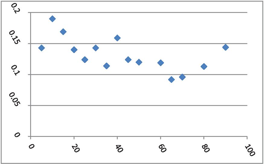
Figure 1 Scatter Plot of data Set-1 with area on X axis and production on y axis.

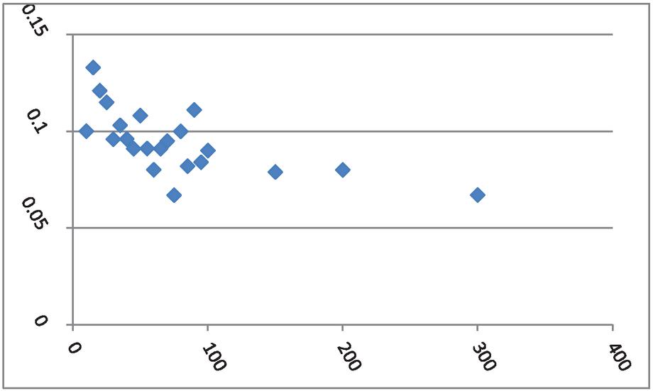
Figure 2 Scatter Plot of data Set-2 with area on X axis and production on y axis.

Table 3 Parameter estimates for various models

Model	a	b	c	d
Model (1)	0.1608	0.9953	–	–
Model (2)	0.2159	$-$ 0.1406	–	–
Model (3)	0.1629	0.0050	–	–
Model (4)	0.1084	0.0718	0.9681	–
Model (5)	$-$ 1.6335	0.0058	1.8141	0.9956
Model (6)	0.1309	$-$ 1.0780	0.3323	0.9285
Model (7)	0.1181	$-$ 3.5015	0.2651	0.9099

Figures 1 and 2 show that a straight line is not the best fit model or curve; instead, the plots show nonlinear patterns. Thus, we seek the best-fitted nonlinear growth model so that the very close estimation of the fitted model’s parameters and the best prediction of the yield of the peppermint may be achieved. The best policies at the block level of the Barabanki district of Uttar Pradesh in India may be made and implemented for the district and state’s economic growth.

To judge the efficiencies of the competing and the introduced models, we have considered two real primary data sets gathered from two blocks of the Barabanki district of Uttar Pradesh in India on peppermint crop yield. The computation on parameters of the models, the models’ adequacy, and residuals analysis for competing and the suggested models (1) to (7) have been carried out. The Estimated values of different parameters for data Set-1 are given in Table 3, while Table 4 represents the values of various measures of goodness of fit for the competing and the suggested estimators. Similarly, data Set-2 is given in Table 5, and various measures of goodness of fit for the competing and the suggested estimators are presented in Table 6.

Table 4 Goodness of fit of models & residuals analysis

	Model (1)	Model (2)	Model (3)	Model (4)	Model (5)	Model (6)	Model (7)
$R^{2}$	0.3787	0.3807	0.3802	0.4446	0.4973	0.6029	0.6146
$R_{A d j}^{2}$	0.3309	0.3331	0.3325	0.3521	0.3602	0.4946	0.5095
$s^{2}$	0.000474	0.000472	0.000473	0.000459	0.000453	0.000358	0.000347
M.A.E.	0.0166	0.0166	0.0166	0.0154	0.0150	0.0124	0.0116
M.A.P.E	12.7083	12.5857	12.6633	11.7003	11.4052	9.9358	9.4138
DW#	1.7233	1.8638	1.7343	1.9236	2.0275	1.7833	1.7945
R*	0.556	0.556	0.556	0.556	0.000	0.000	0.000
	(0.578)	(0.578)	(0.578)	(0.578)	(1.000)	(1.000)	(1.000)
SW^	0. 908	0. 921	0.910	0.921	0.963	0.960	0.946
	(0.128)	(0.203)	(0.134)	(0.199)	(0.749)	(0.692)	(0.465)
# represents values of Durbin & Watson Test, *Values of Run test, ^ Values of Shapiro-Wilk test, the p-values are presented within parentheses.

Table 5 Estimates of different parameters for different models

Model	a	b	c	d
Model (1)	0.1090	0.9980	–	–
Model (2)	0.1717	$-$ 0.1493	–	–
Model (3)	0.1099	0.0020	–	–
Model (4)	0.0704	0.0514	0.9873	–
Model (5)	0.0324	0.00009	0.0864	0.9930
Model (6)	0.0752	$-$ 0.1992	0.0685	0.9811
Model (7)	0.0838	$-$ 6.9171	0.1452	0.9519

Table 6 Goodness of fit of models & residuals analysis

	Model (1)	Model (2)	Model (3)	Model (4)	Model (5)	Model (6)	Model (7)
$R^{2}$	0.4445	0.5118	0.4451	0.5215	0.5089	0.5336	0.5884
$R_{A d j}^{2}$	0.4167	0.4874	0.4173	0.4711	0.4270	0.4559	0.5198
$s^{2}$	0.000158	0.000138	0.000157	0.000143	0.000155	0.000147	0.000130
M.A.E.	0.0093	0.0087	0.0094	0.0088	0.0090	0.0087	0.0076
M.A.P.E	10.0955	9.3459	10.2353	9.4283	9.7328	9.3789	8.4828
DW#	2.0463	2.4577	2.0499	2.4145	2.3610	2.3942	2.3806
R*	1.529	1.966	1.092	1.092	1.529	-0.218	-0.218
	(0.126)	(0.049)	(0.275)	(0.275)	(0.126)	(0.827)	(0.827)
SW^	0.974	0.972	0.979	0.988	0.978	0.986	0.964
	(0.802)	(0.753)	(0.898)	(0.991)	(0.889)	(0.979)	(0.566)
# represents values of Durbin & Watson Test, *Values of Run test, ^ Values of Shapiro-Wilk test, the p-values are presented within parentheses.

7 Results and Discussion

It may be verified from Table 4 that $R^{2}$ for different models under completion lies in between [0.3787 0.4446], while it ranges from [0.4973 0.6146] for the introduced models, respectively. Similarly, $R_{A d j}^{2}$ ranges from [0.3309 0.3521] for the competing models and from [0.3602 0.5095] for the proposed models, respectively. The $s^{2}$ ranges from [0.000459 0.000474] for the models in competition, while it ranges from [0.000347 0.000453] for the introduced models, respectively. The M.A.E. ranges from [0.0154 0.0166] for the models in competition and ranges from [0.0116 0.0150] for the suggested models, respectively. The value of M.A.P.E. ranges from [11.7003 12.7083] for the models in competition while from [9.4138 11.4052] for the introduced models, respectively. Some other measures presented in Table 4, Durbin-Watson statistic, Run-test and Shapiro-Wilk test are appropriate for the introduced models in comparison to the models in competition. Table 6 is also showing similar results for the data set-2 as in Table 4.

Figures 3 and 4 represent the graph of $R^{2}$ , $R_{A d j}^{2}$ , $s^{2}$ , M.A.E. and M.A.P.E. for the proposed and the competing models respectively for given Data Sets.

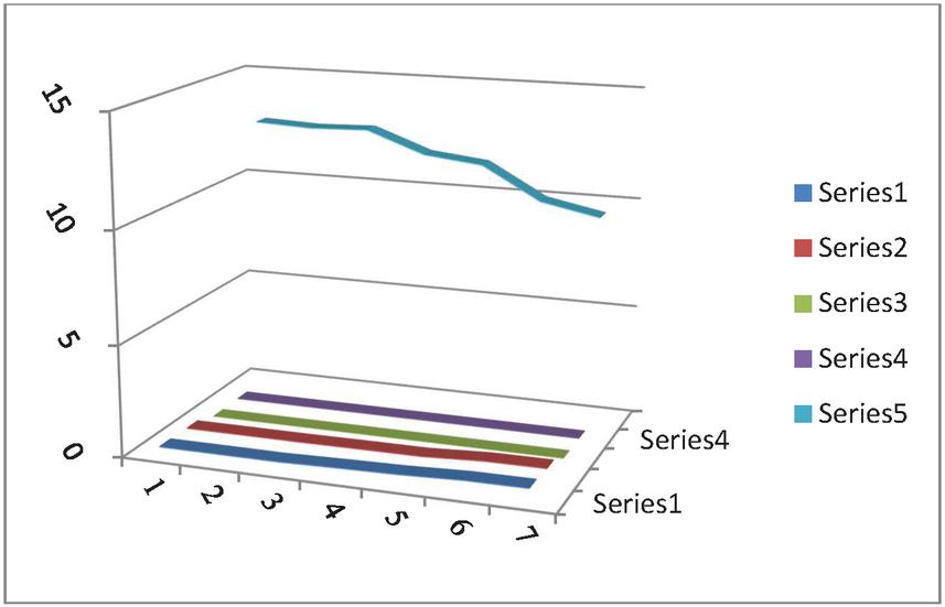
Figure 3 Fitting measures for data set-1.

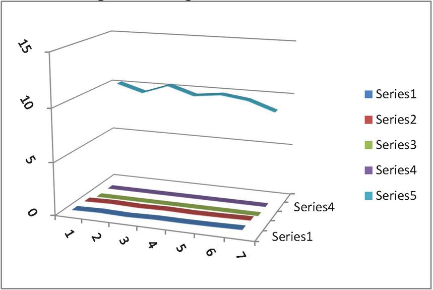
Figure 4 Fitting measures for data set-2.

8 Conclusion

In this paper, we have introduced three new growth models for efficiently estimating and predicting the peppermint crop yield. We have studied the statistical measures of the proposed models. A comparison of the introduced models has been made with the competing growth models based on the fitting measures $R^{2}$ , $R_{A d j}^{2}$ , $s^{2}$ , MAE, MAPE, Durbin-Watson statistic, Run-test, and Shapiro-Wilk test. It can be observed from Tables 4 and 6 that the fitting measures are most appropriate for the proposed models in comparison to the models in competition. As the goodness of fit measure is best for the introduced models compared to competing models, they will estimate and predict better than the competing models. Thus, the proposed models are best for predicting peppermint yield production and may be used in policymaking for peppermint crop production for good yield and market demand and economic benefit to the Barabanki district of India.

The study contributes to the understanding of the seasonal variation in the cultivation and harvesting of peppermint. The understanding of crop rotation as unique to the production of peppermint that help farmers to improve on the increased level of output of their product. Also, because peppermint has medicinal benefits, the provided models could assist the farmers in achieving better optimal production levels in their cultivation. The monitory advantage may also be obtained by maximizing peppermint output from the appropriate area of cultivation, as suggested by the proposed model. The model can also be utilized in other fields of application such as Biological Sciences, Economics, Fisheries, Medical Sciences, Poultry, and so on for different growth variables by incorporating the appropriate explanatory variables. More efficient models for estimating and forecasting peppermint and other crop production may be sought in the near future.

Acknowledgement

The authors would like to express their heartfelt gratitude to the Editor and the knowledgeable referees for their valuable comments, which helped to improve the earlier draft.

References

Al-Kassie, G.A.M. (2010). The role of peppermint (Mentha Piperita) on performance in broiler diets, Agriculture and Biology Journal of North America, 1(5), 1009–1013.

Dharmaraja S., Jain V., Anjoy P. and Chandra H. (2020) Empirical Analysis for Crop Yield Forecasting in India, Agricultural Research, 9(1), 132–138.

Draper, N.R. and Smith, H., Applied Regression Analysis, 3rd Ed., John Wiley & Sons, 1998.

Gujarati, D. N. And Sangeetha, Basic Econometrics, 4th Ed, Tata McGraw-Hill, 2007.

Guo Y., Xiang H., Li Z., Ma F. and Du C. (2021). Prediction of Rice Yield in East China Based on Climate and Agronomic Traits Data Using Artificial Neural Networks and Partial Least Squares Regression, Agronomy, 11(282), 1–11.

Gupta R.P., Rai V.N., Kumar S. and Snehdeep (2021). Statistical models for wheat yield using linear regression model based on meteorological parameters, Journal of Pharmacognosy and Phytochemistry, 10(2), 44–46.

Haque H. N., Azad N. K., Jha R. N. and Singh S. N. (1988). Optimum Size and Shape of Plots for Wheat, Annals of Agricultural Research, 9(2), 165–170.

Kaplan, S. and Gurcan, E.K. (2018). Comparison of growth curves using non-linear regression function in Japanese quail, Journal of Applied Animal Research, 46(1), 112–117.

Kumar, S., Suresh, R., Singh, V. and Singh, A. K. (2011). Economic Analysis of Menthol Mint Cultivation in Uttar Pradesh: A Case Study of Barabanki District, Agricultural Economics Research Review, 24(2), 345–350.

Kumar, R., Upadhyaya, R.K., Venkatesha, K.T., Padalia, R.C., Tiwari, A.K. and Singh, S. (2019). Performance of Different Parts of Planting Materials and Plant Geometry on Oil yield and Suckers Production of Menthol-mint (Mentha Arvensis L.) During Winter Season, International Journal of Current Microbiology and Applied Sciences, 8(1), 1261–1266.

Lavanya M., and Parameswari R. (2020). A Multiple Linear Regressions Model for Crop Prediction with Adam Optimizer and Neural Network Mlraonn, International Journal of Advanced Computer Science and Applications, 11(4), 253–257.

Misra, G.C., Shukla, A.K. and Yadav, S.K. (2009). A comparison of regression methods for improved estimation in sampling, Journal of Reliability and Statistical Studies, 2(2), 85–90.

Misra, G.C., Yadav, S.K., Shukla, A.K. and Bahadur, R. (2010). Use of a non-linear model for improved estimation in cluster sampling, Journal of Reliability and Statistical Studies, 3(2), 73–78.

Montgomery D.C., Peck E.A. and Vining G.C., Introduction to Linear Regression Analysis, 5th Ed., Wiley, 2012.

Murugan R., Thomas F.S., GeethaShree G., Glory S. and Shilpa A. (2020). Linear Regression Approach to Predict Crop Yield, 9(1), 40–44.

Nimase R. G., Kandalkar Y. B. and Bangar Y. C. (2018). Non-linear modelling for estimation of growth curve parameters in Madgyal sheep, Journal of Entomology and Zoology Studies, 6(2), 463–465.

Pardarshi Kisan Seva Yojna, Agriculture Department, Uttar Pradesh, http://upagripardarshi.gov.in/Index.aspx

Ratkowsky D.A., Non-Linear Regression Modeling, Marcel Dekker, New York, 1983.

Ratkowsky D.A., Hand Book of Non-Linear Regression Models, Marcel Dekker, New York, 1989.

Riazoshams H., Midi H. and Ghilagaber G., Robust Nonlinear Regression: with Applications using R, 1st Ed, Wiley, 2019.

Satoh D. (2019). Model selection among growth curve models that have the same number of parameters, Cogent Mathematics & Statistics, 6, 1–17.

Scarneciu, C. C., Sangeorzan, L., Rus, H., Scarneciu, V. D., Varciu, M. S., Andreescu, O. and Scarneciu, I. (2017). Comparison of linear and non-linear regression analysis to determine Pulmonary Pressure in Hyperthyroidism, Pakistan Journal of Medical Sciences, 33(1), 111–120.

Singh, N., Singh, P.K. and Kumar S.S. (2018). Growth Rate of Wheat Crop in Azamgarh Division of Eastern Uttar Pradesh, India, International Journal of Current Microbiology and Applied Sciences, 7(3), 3348–3352.

Smith, H.F. (1938). An empirical law describing heterogeneity in the yields of agricultural crops, Journal of Agricultural Science, 28, 1–23.

Wen Y., Liu K., Liu H., Cao H., Mao H., Dong X. and Yin Z. (2019). Comparison of nine growth curve models to describe growth of partridges (Alectoris Chukar), Journal of Applied Animal Research, 47(1), 195–200.

Young P., and Ord J. (1989). Model selection and estimation for technology growth curves, International Journal of Forecasting, 5, 501–513.

Zhao Z., Li Sh., Huang H., Li Ch., Wang Q. and Xue L. (2015). Comparative Study on Growth and Developmental Model of Indigenous Chicken Breeds in China, Open Journal of Animal Sciences, 5, 219–223.

Biographies

S. K. Yadav is an Associate Professor in the Department of Statistics at the Babasaheb Bhimrao Ambedkar University, Lucknow, UP, India. He earned his MSc and PhD in Statistics from the Lucknow University and has qualified to the National Eligibility Test. He has published 65 papers in national and international journals of repute and two books from an international publisher. He is a referee for 20 reputed international journals. He has presented papers in more than 20 national and international conferences and also delivered invited talks in several conferences.

Dinesh K. Sharma is a Professor of Quantitative Methods and Computer Applications in the Department of Business, Management and Accounting at the University of Maryland Eastern Shore. He earned his MS in Mathematics, MS in Computer Science, PhD in Operations Research, and a second PhD in Management. Professor Sharma has over twenty-eight years of teaching experience, served in numerous committees to supervise PhD students. Professor Sharma’s research interests include supply chain management, healthcare management, portfolio management, and stock market prediction, as well as mathematical programming, sampling, and artificial intelligence techniques. He has more than 225 peer-reviewed journal articles and conference proceedings to his credit, as well as numerous best paper awards. He is the Editor-in-Chief of the Journal of Global Information Technology and the Review of Business and Technology Research.

Ayodele Julius Alade, was the former Dean of the School of Business and Technology at the University of Maryland Eastern Shore. Prior to taking the deanship, he was Chair of the Department of Business, Management, and Accounting at the University of Maryland Eastern Shore as well as a Professor of Production and Operations Management and Quantitative Methods. He is currently a Professor and Director of Microsoft Center at UMES. He received his Ph.D. in Industrial Economics from the University of Utah. He has authored and co-authored numerous scholarly journal articles and abstracts that have been published in national and international journals and has been nominated and received several best paper awards. In his research, he has combined theoretic economics with financial and operations management, using linear and goal programming models. Dr. Alade has been involved in several international research activities and consulting/research engagements in international programs particularly in South Africa.

Alok Kumar Shukla is Assistant Professor of Statistics at D.A-V College, Kanpur, India. He received his Ph.D. degree in Statistics from Kanpur University. He is referee of many reputed national and international journals. His research interests are in sampling theory and regression analysis. He has published many research articles in international journals of repute.

Journal of Reliability and Statistical Studies, Vol. 14, Issue 2 (2021), 451–470.
doi: 10.13052/jrss0974-8024.1424
© 2021 River Publishers