Statistical Inference Under Step Stress Partially Accelerated Life Testing for Adaptive Type-II Progressive Hybrid Censored Data

Mustafa Kamal¹, Ahmadur Rahman^2,*, Shazia Zarrin³ and Haneefa Kausar²

¹Department of Basic Sciences, College of Science and Theoretical Studies, Saudi Electronic University, Dammam, 32256, Kingdom of Saudi Arabia

²Department of Statistics and Operations Research, Aligarh Muslim University, India

³Uttaranchal Unani Medical College and Hospital, Haridwar, India

E-mail: m.kamal@seu.edu.sa; kamal19252003@gmail.com; ahmadur.st@gmail.com; shaziazarrin@gmail.com; haneefakausar445@gmail.com

*Corresponding Author

Received 31 July 2021; Accepted 01 November 2021; Publication 06 December 2021

Abstract

Accelerated life tests (ALTs) are designed to investigate the lifetime of extraordinarily reliable things by exposing them to increased stress levels of stressors such as temperature, voltage, pressure, and so on, in order to cause early breakdowns. The Nadarajah-Haghighi (NH) distribution is of tremendous importance and practical relevance in many real-life scenarios due to its attractive qualities such as its density function always has a zero mode and its hazard rate function can be increasing, decreasing, or constant. In this article, the NH distribution is considered as a lifetime distribution under the step stress partially accelerated life testing (SSPALT) model with adaptive type II progressively hybrid censored samples. The unknown model parameters and acceleration factors are estimated using maximum likelihood estimation (MLE) method assuming that the impact of stress change in SSPALT is explained by a tampered random variable (TRV) model. The Fisher information matrix, which is based on large sample theory, is also constructed and used to produce the approximate confidence intervals (ACIs). Furthermore, two potential optimum test strategies based on the A and D optimality criteria are evaluated. To investigate the performance of the proposed methodologies and statistical assumptions established in this article, extensive simulations using R software have been conducted. Finally, to further illustrate the suggested approach, a real-world example based on the times between breakdowns for a repairable system has been provided.

Keywords: Partially accelerated life testing, Nadarajah-Haghighi distribution, adaptive type-II progressive hybrid censoring, maximum likelihood estimation, simulation study.

1 Introduction

In the disciplines of statistics, reliability, and life testing analysis, there are several discrete and continuous distributions, but the exponential distribution stands out owing to its memory-less properties. As a result, it is used as a reference model in the study of reliability and life testing. Due to the limitations of the exponential distribution in explaining only the constant hazard rate, several extensions of the exponential distribution have been suggested in the literature by many writers for a variety of reasons. Nadarajah and Haghighi (2011) proposed one such extension of the exponential distribution, which is commonly referred to as the NH distribution. In their study, they pointed out that the density function of the NH distribution always has a zero mode. Furthermore, its hazard rate function can be increasing, decreasing, or constant, whereas its density function can be monotonically decreasing while the hazard rate function is still increasing. Because of all these appealing characteristics, the NH distribution may be thought of as a viable alternative to the Weibull, Gamma, and Exponentiated Exponential distributions.

For a random variable T following a NH distribution, the probability density function (PDF), the cumulative distribution function (CDF) and the survival function (SF) are given by

$$f(t;\alpha ,\beta )=\alpha \beta {(1+\beta t)}^{\alpha -1}\mathit{exp}[1-{(1+\beta t)}^{\alpha }],t>0,\alpha >0,\beta >0$$	(1)
$$F(t;\alpha ,\beta )=1-\mathit{exp}[1-{(1+\beta t)}^{\alpha }],t>0,\alpha >0,\beta >0$$	(2)
$$R(t)=\mathit{exp}[1-{(1+\beta t)}^{\alpha }],t>0,\alpha >0,\beta >0$$	(3)

Where $\beta$ and $\alpha$ are the distribution’s scale and shape parameters. The exponential distribution and Weibull may be obtained as special cases of the NH distribution. Also, it has closed forms of survival SF and HRF like the Weibull, making it an excellent choice for lifetime data analysts.

Some recent studies that have been done based on NH distribution are, for example, MirMostafaee et al. (2016) computed the best linear unbiased estimators of the parameters of the distribution using moments of upper record values of NH distribution. Selim (2018), Sana and Faizan (2019), briefly described and compared the different methods of frequentist estimation as well as they obtained BEs using different loss functions and gamma priors. Kamal et al. (2020a) employed a linear combination of NH density to expand the NH distribution to a four-parameter distribution, and then looked at a variety of statistical and mathematical characteristics, as well as the MLE method for estimating the parameters. Minic (2020) discussed the procedure for obtaining the estimates of parameters using different methods of estimation and compared them using their biases and mean square errors (MSEs). For complete data, Kamal et al. (2020b) estimated the MLEs of the parameters of the NH distribution using SSALT.

Due to the continuous improvement in research and development in manufacturing industries and the high competition among them to launch their products within a short time period, the reliability of the products has improved significantly in the modern era of technological breakthroughs. Therefore, if one tries to test the life of the products using traditional life testing procedures, it will be a very time consuming and costly process to obtain the required failure data to make an efficient prediction about the product’s lifetimes. So, some special type of testing which can induce required failures quickly is needed and the answer is ALTs and PALTs. ALTs were developed in the literature to explore the lifespan of exceptionally reliable objects by subjecting them to accelerated stress levels of stressors such as temperature, voltage, pressure, and so on, in order to produce early breakdowns. There are numerous models under ALTs that are based on different forms of stress loading, and the most commonly used types are the constant-stress and the step-stress models. Each sample of tested products are subjected to some constant levels of constant stress in a constant-stress model until either all units fail or the test is terminated for some reason such as censoring scheme. Such constant-stress ALT models have been extensively addressed by a number of authors. See, for example, Kamal et al. (2013a), Rahman et al. (2020), Hakamipour (2021), Zhang et al. (2021), Kamal (2021), and Abd El-Raheem (2021) among others, for recent additions. While the test conditions associated with step-stress models do not remain constant throughout the test, they do change at each specified time or when a specified number of failures occurs, implying that the stress on a sample of test units does not remain constant but increases step by step at a prescribed period or simultaneously when a fixed number of failures occurs. Several writers investigated step-stress models as well. For example, Saxena et al. (2012), Kamal et al. (2013b), Hakamipour (2020), Khan and Chandra (2021), Amleh and Raqab (2021) and others.

In ALT, the breakdown information received under accelerated conditions is examined and extrapolated to normal stress levels using a suitable physical model. In some cases, constructing a proper physical model to describe the life stress connection is difficult, if not impossible. The PALT is a superior option to doing live tests in these scenarios. PALTs, like ALTs, are divided into two kinds depending on various types of stress loading: constant-stress and step-stress models. In a constant-stress PALT model, each sample of tested items is subjected to normal and accelerated levels of constant stress until all units fail or the test is discontinued for some reason, such as a censoring scheme. Some relevant references based on the constant-stress PALT model include Zarrin et al. (2012), Kamal et al. (2013c), Hassan et al. (2020) and Rabie (2021). In SSPALT, certain items or materials are initially tested at normal or usage conditions for a predetermined period of time, after which all surviving items or systems are subjected to accelerated test conditions until the termination time. So far, several writers have addressed SSPALT analysis; for example, Goel (1971) presented the TRV model, and DeGroot and Goel (1979) analysed the optimum design of a PALT within a Bayesian decision theory framework based on the TRV model. SSPALT is also considered by Bai and Chung (1992), Bai et al. (1993), Rahman et al. (2016), and Rahman et al. (2019) who use different lifetime distribution and censoring algorithms.

Due to time and cost restrictions in life-testing and reliability experiments, researchers typically trim their data using two of the most commonly used techniques classified as Type-I and Type-II censoring practices. Experiments with Type-I or time censoring schemes have to be terminated by a predetermined time, while in Type-II or Failure censored scheme, life tests are terminated when a certain number of failures are reached. Epstein (1954) proposed a more practicable approach known as a hybrid censorship scheme, which is in fact a logical combination of Type-I and Type-II censorship techniques. It is currently a well-known and widely used method among scholars such as Banerjee and Kundu (2008) and Balakrishnan and Kundu (2013), all of whom have made major contributions to the field of reliability and life testing. All of the above methods lack the ability to delete items during testing. To deal with this scenario, a more effective and adaptable technique known as progressive censoring was devised, which allows the deletion of experimental units throughout the test at various intermittent intervals of time. For further information on the theory, methodology, and applications of progressive censoring, see Balakrishnan (2007) and Balakrishnan and Cramer (2014).

In progressively Type-II hybrid censoring, the number of failures required and the number of items that need to be removed during the experiment are fixed in advance, but there is no constraint on experiment time. Due to this reason, the experiment can be very lengthy. In order to tackle this issue, Kundu and Joarder (2006) introduced a new censoring scheme called the Type-I Progressive Hybrid Censoring Scheme (T-I PHCS) with an additional time and failure constraint that the experiment will run until a pre-specified time point or up to a pre-specified number of failures, whichever comes first. However, the sample size in T-I PHCS is random and only a few failures or even no failures would occur before the pre-specified time limit, which results in lower efficiency of the estimates of the parameters. To resolve the limitation of the T-I PHCS, Ng et al. (2009) proposed an adaptive type-II PHCS in which$n$ units are placed on a life test with a predetermined number of failures $m$ and a pre-fixed progressive censoring scheme ${\xi }_1,{\xi }_2,\mathrm{\dots },{\xi }_m$ but experimenter is allowed to change the values of some of the ${\xi }_{iS}$ during the experiment according to the situation. At first failure time $y_{1,m,n},{\xi }_1$ test items are separated from the experiment at random from the remaining $n-1$ alive items. At second failure time $y_{2,m,n},{\xi }_2$ units of the remaining $n-1-{\xi }_1$ units are randomly removed and so on. If $m^{th}$ failure time $y_{m,m,n}$ occurs before pre-specified time $\eta$, all the remaining ${\xi }_m=n-m-{\sum }_{i=1}^m{\xi }_i$ units are removed and the experiment stops at time $y_{m,m,n}$. In AT-II PHCS, the experiment is allowed to run over the test termination time limit $\eta$. Therefore, if $y_{m,m,n}>\eta$, then the experiment will be terminated as soon as possible by setting ${\xi }_{c+1},{\xi }_{c+2},\mathrm{\dots },{\xi }_{m-1}=0$. This means that if $y_{c,m,n}<\eta <y_{c+1,m,n}$, where $c+1<m$ and $x_{c,m,n}$ is the $c^{th}$ failure time which is occurred before time $\eta$, no surviving item will be removed from the experiment until the effective sample of $m$ failures is obtained and then all of the remaining units ${\xi }_m=n-c-{\sum }_{i=1}^c{\xi }_i$, are removed from the experiment.

So far, many scholars have been considered SSPALT using AT-II PHCS. Lin et al. (2009) discussed the MLEs and approximate MLEs of Weibull parameters and then compared the efficiency of the estimates under two PHCS. Hemmati and Khorram (2013) obtained MLEs and AMLEs of the parameters of log-normal distribution using AT-II PHCS and then compared the results with Type-II PHCS through a simulation study. Ismail (2014) obtained and compered the MLEs of Weibull distribution parameters based on two different types of PHCS. Sobhi and Soliman (2015) dealt with the problem of SSPALT based on AT-II PHCS and obtained the MLEs and BEs of the parameters of the exponentiated Weibull distributions. Assuming the TRV model, Zhang and Shi (2016) discuss the MLEs of the unknown parameters of the extended Weibull distribution. Nassar et al. (2017) investigated the MLEs of the parameters of the Burr Type-XII distribution and compared the results based on two different PHCS. Selim (2018) analysed the parameters of exponentiated exponential distribution under step stress accelerated life testing plans with type-II PHCS. Alam and Ahmed (2020) investigated the MLEs of Exponentiated Pareto distribution under SSPALT using AT-II PHCS.

Motivated by the fact that the NH distribution is of extreme importance and practical relevance in many real-life situations, and since no study has been done based on AT-II PHCS to obtain estimates of the parameters of the NH distribution under SSPALT, the main goal of this study is to obtain the MLEs of the parameters of the NH distribution and the acceleration factors under SSALT based on AT-II PHCS. The remainder of this work is structured as follows. Section 2 discusses fundamental assumptions and the testing procedure. Point estimates, the observed Fisher information matrix, and asymptotic confidence intervals are produced in Section 3. Section 4 discusses optimum test strategies based on A and D optimality. To assess the performance of the estimations in Section 5, a simulation exercise is carried out. Section 6 discusses a real-world case to further illustrate the proposed technique. Section 7 concludes the paper with some results-based discussion.

2 Test Assumptions and Procedure

i. Test is based on simple SSPALT and used only two stress levels $S_u$ (Normal operating conditions) and $S_a$ (Accelerated condition) such that $S_u<S_a$. There should be at least one failure occurs under each stress levels $S_u$ and $S_a$.

ii. The failures of the test items at both stress levels $S_u$ and $S_a$ follow the NH distribution given by (1).

iii. The lifetime $Y$ of the tested item in SSPALT follows a TRV model which is given by

$$Y=\{\begin{array}{cc}\hfill T,\hfill & \text{if}T<\tau \hfill \\ \hfill \tau +\frac{(T-\tau )}{\theta },\hfill & \text{if}T>\tau \hfill \end{array}$$

(4)

where $T$ represents item’s lifetime under stress $S_u$, $\tau$ represents the time point when stress is change to $S_a$ from $S_u$ and $\theta >1$ is an accelerated factor (AF).

Using TRV model, PDF, CDF and RF at stress $S_u$ are obtained as follows

$$f_u(y;\alpha ,\beta )=\alpha \beta {(1+\beta y)}^{\alpha -1}\mathit{exp}[1-{(1+\beta y)}^{\alpha }]$$	(5)
$$F_u(y;\alpha ,\beta )=1-\mathit{exp}[1-{(1+\beta y)}^{\alpha }]$$	(6)
$$R_u(y)=\mathit{exp}[1-{(1+\beta y)}^{\alpha }]$$	(7)

and now, PDF, CDF and RF at stress $S_a$ are obtained as follows

$$f_a(y)=\alpha \beta \theta {[1+\beta (\tau +\theta (y-\tau ))]}^{\alpha -1}\mathit{exp}[1-{\{1+\beta (\tau +\theta (y-\tau ))\}}^{\alpha }]$$	(8)
$$F_a(y)=1-\mathit{exp}[1-{\{1+\beta (\tau +\theta (y-\tau ))\}}^{\alpha }]$$	(9)
$$R_a(y)=\mathit{exp}[1-{\{1+\beta (\tau +\theta (y-\tau ))\}}^{\alpha }]$$	(10)

The test based on SSPALT to obtain the failure data under AT-II PHCS will proceed as follows:

Assume a sample of $n$ items is allocated to the stress level $S_u$ to test under SSPALT with a known progressive censoring scheme ${\xi }_1,{\xi }_2,\mathrm{\dots },{\xi }_m$. Now test will progress and the items out of $n$ that do not fail up to time $\tau$ under $S_u$ are placed through the stress level $S_a$ to test, and the test will continue until censorship time $\eta$ is reached. If the $m^{th}$ failure does not occur within censoring point $\eta$, none of the items is omitted out from test. The testing will continue unless $m^{th}$ failure is recorded, at which point it will be stopped after eliminating all remaining items. As a result, the implemented scheme in this case becomes ${\xi }_1,{\xi }_2,\mathrm{\dots },{\xi }_c,0,0,\mathrm{\dots },0,{\xi }_m$, and then we will acquire the observed sample in the form shown below:

$y_{1,m,n}<y_{2,m,n}<\mathrm{\cdots }<y_{m_u,m,n}$	$\le \tau <y_{m_u+1,m,n}<\mathrm{\cdots }<y_{c,m,n}$
	$<\eta <y_{c+1,m,n}<\mathrm{\cdots }<y_{m,m,n}$

Conventional type-II censoring scheme is a special case of the AT-II PHCS for $\eta \to 0$, and AT-II PHCS reduced to the classical Type-II PHCS if $\eta \to \mathrm{\infty }$.

3 The ML Estimation Procedure of the Model Parameters

In this section, estimates of unknown model parameters and the acceleration factor are obtained by the MLE method. This is a more robust and efficient method that yields estimates with good statistical properties and quantifies uncertainty through confidence limits.

The likelihood function for SSALT with AT-II PHCS data can be written as follows:

$L(y,\alpha ,\beta ,\theta )\propto {\displaystyle \prod _{i=1}^{m_u}}{f}_u(y_i){[R_u(y_i)]}^{{\xi }_i}{\displaystyle \prod _{i=m_u+1}^m}{f}_a(y_i){[R_a(y_i)]}^{{\xi }_i}{[R_a(y_m)]}^{{\xi }_m}$

(11)

Where, $y_i=y_{i,m,n};{\xi }_m=n-m-{\sum }_{i=1}^c{\xi }_i$

$L(y,\alpha ,\beta ,\theta )$	$\propto {\displaystyle \prod _{i=1}^{m_u}}\alpha \beta {(1+\beta y_i)}^{\alpha -1}exp\{1-{⟨1+\beta y_i⟩}^{\alpha }\}$
	$\mathrm{\hspace{1em}}\times {[exp\{1-{⟨1+\beta y_i⟩}^{\alpha }\}]}^{{\xi }_i}$
	$\mathrm{\hspace{1em}}\times {\displaystyle \prod _{i=m_u+1}^m}\alpha \theta \beta {\{1+\beta (\tau +\theta (y_i-\tau ))\}}^{\alpha -1}$
	$\mathrm{\hspace{1em}}\times exp\{1-{⟨1+\beta (\tau +\theta (y_i-\tau ))⟩}^{\alpha }\}$
	$\mathrm{\hspace{1em}}\times {[exp\{1-{⟨1+\beta (\tau +\theta (y_i-\tau ))⟩}^{\alpha }\}]}^{{\xi }_i}$
	$\mathrm{\hspace{1em}}\times {[exp\{1-{⟨1+\beta (\tau +\theta (y_m-\tau ))⟩}^{\alpha }\}]}^{{\xi }_m}$	(12)

By taking natural logarithm on both side of the Equation (12), we get log-likelihood equation $L(y,\alpha ,\beta ,\theta )=\mathrm{\ell }$ as follows

$\mathrm{\ell }$	$=m(log\alpha +log\beta )+(m-m_u)log\theta -(m-m_u){\xi }_m$
	$\mathrm{\hspace{1em}}\times [1-{\{1+\beta (\tau +\theta (y_m-\tau ))\}}^{\alpha }]$
	$\mathrm{\hspace{1em}}+(\alpha -1){\displaystyle \sum _{i=1}^{m_u}}\log (1+\beta y_i)+{\displaystyle \sum _{i=1}^{m_u}}(1+{\xi }_i)\{1-{(1+\beta y_i)}^{\alpha }\}$
	$\mathrm{\hspace{1em}}+(\alpha -1){\displaystyle \sum _{i=m_u+1}^m}\log \{1+\beta ⟨\tau +\theta (y_i-\tau )⟩\}$
	$\mathrm{\hspace{1em}}+{\displaystyle \sum _{i=m_u+1}^m}(1+{\xi }_i)[1-{\{1+\beta (\tau +\theta (y_i-\tau ))\}}^{\alpha }]$	(13)

3.1 Point Estimates

The MLEs of the parameters $\alpha ,\beta$ and $\theta$ can be obtained by solving the following equations:

${\displaystyle \frac{\partial l}{\partial \alpha }}$	$={\displaystyle \frac{m}{\alpha }}-(m-m_u){\xi }_m{\{1+\beta (\tau +\theta (y_m-\tau ))\}}^{\alpha }$
	$\mathrm{\hspace{1em}}\times log\{1+\beta (\tau +\theta (y_m-\tau ))\}+{\displaystyle \sum _{i=1}^{m_u}}log(1+\beta y_i)$
	$\mathrm{\hspace{1em}}-{\displaystyle \sum _{i=1}^{m_u}}(1+{\xi }_i){(1+\beta y_i)}^{\alpha }log(1+\beta y_i)$
	$\mathrm{\hspace{1em}}+{\displaystyle \sum _{i=m_u+1}^m}log\{1+\beta (\tau +\theta (y_i-\tau ))\}$
	$\mathrm{\hspace{1em}}-{\displaystyle \sum _{i=m_u+1}^m}(1+{\xi }_i){\{1+\beta (\tau +\theta (y_i-\tau ))\}}^{\alpha }$
	$\mathrm{\hspace{1em}}\times log\{1+\beta (\tau +\theta (y_i-\tau ))\}$	(14)
${\displaystyle \frac{\partial l}{\partial \beta }}$	$={\displaystyle \frac{m}{\beta }}-(m-m_u){\xi }_m\alpha (\tau +\theta (y_m-\tau )){\{1+\beta (\tau +\theta (y_m-\tau ))\}}^{\alpha -1}$
	$\mathrm{\hspace{1em}}+(\alpha -1){\displaystyle \sum _{i=1}^{m_u}}{\displaystyle \frac{y_i}{(1+\beta y_i)}}-\alpha {\displaystyle \sum _{i=1}^{m_u}}(1+{\xi }_i){(1+\beta y_i)}^{\alpha -1}$
	$\mathrm{\hspace{1em}}+{\displaystyle \sum _{i=m_u+1}^m}{\displaystyle \frac{\tau +\theta (y_i-\tau )}{\{1+\beta (\tau +\theta (y_i-\tau ))\}}}$
	$\mathrm{\hspace{1em}}-\alpha {\displaystyle \sum _{i=m_u+1}^m}(1+{\xi }_i)(\tau +\theta (y_i-\tau )){\{1+\beta (\tau +\theta (y_i-\tau ))\}}^{\alpha -1}$	(15)
${\displaystyle \frac{\partial l}{\partial \theta }}$	$={\displaystyle \frac{(m-m_u)}{\theta }}-(m-m_u){\xi }_m\beta (y_m-\tau ){\{1+\beta (\tau +\theta (y_m-\tau ))\}}^{\alpha -1}$
	$\mathrm{\hspace{1em}}+(\alpha -1)\beta {\displaystyle \sum _{i=m_u+1}^m}{\displaystyle \frac{(y_i-\tau )}{\{1+\beta (\tau +\theta (y_i-\tau ))\}}}$
	$\mathrm{\hspace{1em}}-\alpha \beta {\displaystyle \sum _{i=m_u+1}^m}(1+{\xi }_i)(y_i-\tau ){\{1+\beta (\tau +\theta (y_i-\tau ))\}}^{\alpha -1}=0$	(16)

Equations (14), (15) and (16) are non-linear equations and have no closed form solution. Some iterative techniques, such as Newton-Raphson techniques, can therefore be used to obtain a numerical solution of the estimates.

3.2 Derivation of Fisher’s Information Matrix

The observed FIM can be derived as follows

$$\mathit{FIM}=-\left[\begin{array}{ccc}\hfill \frac{{\partial }^2\mathrm{\ell }}{\partial {\alpha }^2}\mathit{\hspace{1em}}\hfill & \hfill \frac{{\partial }^2\mathrm{\ell }}{\partial \alpha \partial \beta }\mathit{\hspace{1em}}\hfill & \hfill \frac{{\partial }^2\mathrm{\ell }}{\partial \alpha \partial \theta }\hfill \\ \hfill \frac{{\partial }^2\mathrm{\ell }}{\partial \beta \partial \alpha }\mathit{\hspace{1em}}\hfill & \hfill \frac{{\partial }^2\mathrm{\ell }}{\partial {\beta }^2}\mathit{\hspace{1em}}\hfill & \hfill \frac{{\partial }^2\mathrm{\ell }}{\partial \beta \partial \theta }\hfill \\ \hfill \frac{{\partial }^2\mathrm{\ell }}{\partial \theta \partial \alpha }\mathit{\hspace{1em}}\hfill & \hfill \frac{{\partial }^2\mathrm{\ell }}{\partial \theta \partial \beta }\mathit{\hspace{1em}}\hfill & \hfill \frac{{\partial }^2\mathrm{\ell }}{\partial {\theta }^2}\hfill \end{array}\right]$$

Where, $\frac{{\partial }^2\mathrm{\ell }}{\partial \alpha \partial \beta }=\frac{{\partial }^2\mathrm{\ell }}{\partial \beta \partial \alpha }$; $\frac{{\partial }^2\mathrm{\ell }}{\partial \beta \partial \theta }=\frac{{\partial }^2\mathrm{\ell }}{\partial \theta \partial \beta }$; and $\frac{{\partial }^2\mathrm{\ell }}{\partial \alpha \partial \theta }=\frac{{\partial }^2\mathrm{\ell }}{\partial \theta \partial \alpha }$, now elements of the FIM are given by following equation:

${\displaystyle \frac{{\partial }^{2}l}{\partial {\alpha }^2}}$	$=-{\displaystyle \frac{m}{{\alpha }^2}}-(m-m_u){\xi }_m{\{1+\beta (\tau +\theta (y_m-\tau ))\}}^{\alpha }$
	$\mathrm{\hspace{1em}}\times {[log\{1+\beta (\tau +\theta (y_m-\tau ))\}]}^2$
	$\mathrm{\hspace{1em}}-{\displaystyle \sum _{i=1}^{m_u}}(1+{\xi }_i){(1+\beta y_i)}^{\alpha }{\{log(1+\beta y_i)\}}^2$
	$\mathrm{\hspace{1em}}-{\displaystyle \sum _{i=m_u+1}^m}(1+{\xi }_i){\{1+\beta (\tau +\theta (y_i-\tau ))\}}^{\alpha }$
	$\mathrm{\hspace{1em}}\times {[log\{1+\beta (\tau +\theta (y_i-\tau ))\}]}^2$	(17)
${\displaystyle \frac{{\partial }^{2}l}{\partial {\beta }^2}}$	$=-{\displaystyle \frac{m}{{\beta }^2}}-(m-m_u){\xi }_m\alpha (\alpha -1){(\tau +\theta (y_m-\tau ))}^2$
	$\mathrm{\hspace{1em}}\times {\{1+\beta (\tau +\theta (y_m-\tau ))\}}^{\alpha -1}-(\alpha -1){\displaystyle \sum _{i=1}^{m_u}}{\displaystyle \frac{y_i{}^2}{{(1+\theta y_i)}^2}}$
	$\mathrm{\hspace{1em}}-\alpha (\alpha -1){\displaystyle \sum _{i=1}^{m_u}}(1+{\xi }_i)y_i{}^2{(1+\beta y_i)}^{\alpha -2}$
	$\mathrm{\hspace{1em}}-(\alpha -1){\displaystyle \sum _{i=m_u+1}^m}{\displaystyle \frac{{(\tau +\theta (y_i-\tau ))}^2}{{\{1+\beta (\tau +\theta (y_i-\tau ))\}}^2}}$
	$\mathrm{\hspace{1em}}-\alpha (\alpha -1){\displaystyle \sum _{i=m_u+1}^m}(1+{\xi }_i){(\tau +\theta (y_i-\tau ))}^2$
	$\mathrm{\hspace{1em}}\times {\{1+\beta (\tau +\theta (y_i-\tau ))\}}^{\alpha -2}$	(18)
${\displaystyle \frac{{\partial }^{2}l}{\partial {\theta }^2}}$	$=-{\displaystyle \frac{(m-m_u)}{{\theta }^2}}-(m-m_u){\xi }_m\alpha (\alpha -1){\beta }^2{(y_m-\tau )}^2$
	$\mathrm{\hspace{1em}}\times {\{1+\beta (\tau +\theta (y_m-\tau ))\}}^{\alpha -2}$
	$\mathrm{\hspace{1em}}-(\alpha -1){\beta }^2{\displaystyle \sum _{i=m_u+1}^m}{\displaystyle \frac{{(y_i-\tau )}^2}{{\{1+\beta (\tau +\theta (y_i-\tau ))\}}^2}}$
	$\mathrm{\hspace{1em}}-\alpha (\alpha -1){\beta }^2{\displaystyle \sum _{i=m_u+1}^m}(1+{\xi }_i){(y_i-\tau )}^2$
	$\mathrm{\hspace{1em}}\times {\{1+\beta (\tau +\theta (y_i-\tau ))\}}^{\alpha -2}$	(19)
${\displaystyle \frac{{\partial }^{2}l}{\partial \alpha \partial \beta }}$	$={\displaystyle \frac{{\partial }^{2}l}{\partial \beta \partial \alpha }}=-(m-m_u){\xi }_m(\tau +\theta (y_m-\tau ))$
	$\mathrm{\hspace{1em}}\times {\{1+\beta (\tau +\theta (y_m-\tau ))\}}^{\alpha -1}$
	$\mathrm{\hspace{1em}}\times [1+\alpha log\{1+\beta (\tau +\theta (y_m-\tau ))\}]+{\displaystyle \sum _{i=1}^{m_u}}{\displaystyle \frac{y_i}{(1+\beta y_i)}}$
	$\mathrm{\hspace{1em}}-{\displaystyle \sum _{i=1}^{m_u}}(1+{\xi }_i)y_i{(1+\beta y_i)}^{\alpha -1}\{1+\alpha log(1+\beta y_i)\}$
	$\mathrm{\hspace{1em}}+{\displaystyle \sum _{i=m_u+1}^m}{\displaystyle \frac{\tau +\theta (y_i-\tau )}{\{1+\beta (\tau +\theta (y_i-\tau ))\}}}$
	$\mathrm{\hspace{1em}}-{\displaystyle \sum _{i=m_u+1}^m}(1+{\xi }_i)(\tau +\theta (y_i-\tau ))$
	$\mathrm{\hspace{1em}}\times {\{1+\beta (\tau +\theta (y_i-\tau ))\}}^{\alpha -1}$
	$\mathrm{\hspace{1em}}\times [1+\alpha log\{1+\beta (\tau +\theta (y_i-\tau ))\}]$	(20)
${\displaystyle \frac{{\partial }^{2}l}{\partial \beta \partial \theta }}={\displaystyle \frac{{\partial }^{2}l}{\partial \theta \partial \beta }}$	$=-(m-m_u){\xi }_m\alpha (y_m-\tau ){\{1+\beta (\tau +\theta (y_m-\tau ))\}}^{\alpha -2}$
	$\mathrm{\hspace{1em}}\times [1+\alpha \beta (\tau +\theta (y_m-\tau ))]+(\alpha -1)$
	$\mathrm{\hspace{1em}}\times {\displaystyle \sum _{i=m_u+1}^m}{\displaystyle \frac{(y_i-\tau )}{{\{1+\beta (\tau +\theta (y_i-\tau ))\}}^2}}$
	$\mathrm{\hspace{1em}}+\alpha {\displaystyle \sum _{i=m_u+1}^m}(1+{\xi }_i)(y_i-\tau ){\{1+\beta (\tau +\theta (y_i-\tau ))\}}^{\alpha -2}$
	$\mathrm{\hspace{1em}}\times \{1+\alpha \beta (\tau +\theta (y_i-\tau ))\}$	(21)
${\displaystyle \frac{{\partial }^{2}l}{\partial \alpha \partial \theta }}={\displaystyle \frac{{\partial }^{2}l}{\partial \theta \partial \alpha }}$	$=-(m-m_u){\xi }_m\beta (y_m-\tau ){\{1+\beta (\tau +\theta (y_m-\tau ))\}}^{\alpha -1}$
	$\mathrm{\hspace{1em}}\times [1+\alpha log\{1+\beta (\tau +\theta (y_m-\tau ))\}]$
	$\mathrm{\hspace{1em}}+\beta {\displaystyle \sum _{i=m_u+1}^m}{\displaystyle \frac{(y_i-\tau )}{\{1+\beta (\tau +\theta (y_i-\tau ))\}}}$
	$\mathrm{\hspace{1em}}-{\displaystyle \sum _{i=m_u+1}^m}(1+{\xi }_i)(y_i-\tau ){\{1+\beta (\tau +\theta (y_i-\tau ))\}}^{\alpha -1}$
	$\mathrm{\hspace{1em}}\times [1+\alpha log\{1+\beta (\tau +\theta (y_i-\tau ))\}]$	(22)

3.3 Confidence Interval Estimates

As we know that the MLEs of the parameters are distributed approximately according to normal distribution with mean $(\alpha ,\beta ,\theta )$ and variance ${(\mathit{FIM})}^{-1}$ as $n\to \mathrm{\infty }$, therefore, $(\widehat{\alpha },\widehat{\beta },\widehat{\theta })\sim N((\alpha ,\beta ,\theta ),{(FIM)}^{-1})$, where, ${(\mathit{FIM})}^{-1}$ stands for inverse of observed FIM. Now, two sided $100(1-\delta )\%$ approximate confidence interval for the parameter $(\alpha ,\beta ,\theta )$ can be obtained as

$$\widehat{\alpha }\pm Z_{\delta /2}\sqrt{var(\widehat{\alpha })};\widehat{\beta }\pm Z_{\delta /2}\sqrt{var(\widehat{\beta })};\widehat{\theta }\pm Z_{\delta /2}\sqrt{var(\widehat{\theta })}$$

Where $Z_{\delta /2}$ is the ${(1-\delta /2)}^{th}$ quantile of a standard normal distribution and $\sqrt{var(\widehat{\alpha })}$, $\sqrt{var(\widehat{\beta })}$ and $\sqrt{var(\widehat{\theta })}$ are asymptotic variances of $\widehat{\alpha },\widehat{\beta }$ and $\widehat{\theta }$ respectively and are obtained by taking the square root of the diagonal elements of ${(\mathit{FIM})}^{-1}$. By taking the inverse of FIM, we obtain VC matrix as follows

${(\mathit{FIM})}^{-1}$

$={\left[\begin{array}{ccc}\hfill {\displaystyle \frac{{\partial }^2\mathrm{\ell }}{\partial {\alpha }^2}}\mathit{\hspace{1em}}\hfill & \hfill {\displaystyle \frac{{\partial }^2\mathrm{\ell }}{\partial \alpha \partial \beta }}\mathit{\hspace{1em}}\hfill & \hfill {\displaystyle \frac{{\partial }^2\mathrm{\ell }}{\partial \alpha \partial \theta }}\hfill \\ \hfill {\displaystyle \frac{{\partial }^2\mathrm{\ell }}{\partial \beta \partial \alpha }}\mathit{\hspace{1em}}\hfill & \hfill {\displaystyle \frac{{\partial }^2\mathrm{\ell }}{\partial {\beta }^2}}\mathit{\hspace{1em}}\hfill & \hfill {\displaystyle \frac{{\partial }^2\mathrm{\ell }}{\partial \beta \partial \theta }}\hfill \\ \hfill {\displaystyle \frac{{\partial }^2\mathrm{\ell }}{\partial \theta \partial \alpha }}\mathit{\hspace{1em}}\hfill & \hfill {\displaystyle \frac{{\partial }^2\mathrm{\ell }}{\partial \theta \partial \beta }}\mathit{\hspace{1em}}\hfill & \hfill {\displaystyle \frac{{\partial }^2\mathrm{\ell }}{\partial {\theta }^2}}\hfill \end{array}\right]}_{\alpha =\widehat{\alpha },\beta =\widehat{\beta },\theta =\widehat{\theta }}^{-1}$

$=\left[\begin{array}{ccc}\hfill var(\widehat{\alpha })\mathit{\hspace{1em}}\hfill & \hfill covar(\widehat{\alpha }\beta )\mathit{\hspace{1em}}\hfill & \hfill covar(\widehat{\alpha }\theta )\hfill \\ \hfill covar(\widehat{\beta }\widehat{\alpha })\mathit{\hspace{1em}}\hfill & \hfill var(\widehat{\beta })\mathit{\hspace{1em}}\hfill & \hfill covar(\widehat{\beta }\theta )\hfill \\ \hfill covar(\widehat{\theta }\widehat{\alpha })\mathit{\hspace{1em}}\hfill & \hfill covar(\widehat{\theta }\widehat{\beta })\mathit{\hspace{1em}}\hfill & \hfill var(\widehat{\theta })\hfill \end{array}\right]$

4 Optimization of Test Plan Using A and D Technique

4.1 A-optimality Criterion (or Trace Criterion)

The first optimality criteria we employed here is A-optimality, which is obtained by minimizing the trace of the variance-covariance matrix. This may be done mathematically as follows:

$$\mathit{\text{Minimize}}[tr{(\mathit{\text{FIM}})}^{-1}]=[var(\alpha )+var(\beta )+var(\theta )]$$

4.2 Optimum Test Plans using D-optimality Criterion

Another SSPALT optimality criteria is to determine the appropriate time to transition stress from a regular to an accelerated state. The D-optimality criterion is utilized to calculate the optimal stress shift time $\tau$ in this work. It is based on the generalized asymptotic variance (GAV), which is proportional to the reciprocal of the FIM determinant and takes into consideration the whole parameter space. As a result, maximization of the FIM determinant corresponds to GAV minimization. The D-optimality function can be expressed as follows:

$$\mathit{GAV}(\widehat{\alpha },\widehat{\beta },\widehat{\theta })=\frac{1}{det(FIM)}\mathit{\hspace{1em}}\mathit{or}\mathit{\hspace{1em}}\frac{1}{|\mathit{FIM}|}$$

Where $|\mathit{FIM}|$ can be obtained as follows:

$|\mathit{FIM}|$	$=\{({\displaystyle \frac{{\partial }^{2}l}{\partial {\alpha }^2}}\times {\displaystyle \frac{{\partial }^{2}l}{\partial {\beta }^2}}\times {\displaystyle \frac{{\partial }^{2}l}{\partial {\beta }^2}})+({\displaystyle \frac{{\partial }^{2}l}{\partial \alpha \partial \beta }}\times {\displaystyle \frac{{\partial }^{2}l}{\partial \beta \partial \theta }}\times {\displaystyle \frac{{\partial }^{2}l}{\partial \theta \partial \alpha }})$
	$+({\displaystyle \frac{{\partial }^{2}l}{\partial \alpha \partial \theta }}\times {\displaystyle \frac{{\partial }^{2}l}{\partial \beta \partial \alpha }}\times {\displaystyle \frac{{\partial }^{2}l}{\partial \theta \partial \beta }})\}$
	$\mathrm{\hspace{1em}}-\{({\displaystyle \frac{{\partial }^{2}l}{\partial \theta \partial \alpha }}\times {\displaystyle \frac{{\partial }^{2}l}{\partial {\beta }^2}}\times {\displaystyle \frac{{\partial }^{2}l}{\partial \alpha \partial \theta }})+({\displaystyle \frac{{\partial }^{2}l}{\partial \theta \partial \beta }}\times {\displaystyle \frac{{\partial }^{2}l}{\partial \beta \partial \theta }}\times {\displaystyle \frac{{\partial }^{2}l}{\partial {\alpha }^2}})$
	$+({\displaystyle \frac{{\partial }^{2}l}{\partial {\theta }^2}}\times {\displaystyle \frac{{\partial }^{2}l}{\partial \beta \partial \alpha }}\times {\displaystyle \frac{{\partial }^{2}l}{\partial \alpha \partial \beta }})\}$
	$=\left\{{\mathrm{e}}_{\alpha \alpha }{\mathrm{e}}_{\beta \beta }{\mathrm{e}}_{\theta \theta }+2{\mathrm{e}}_{\alpha \beta }{\mathrm{e}}_{\alpha \theta }{\mathrm{e}}_{\beta \theta }\right\}-\left\{e_{\alpha \theta }^2{\mathrm{e}}_{\beta \beta }+e_{\beta \theta }^2{\mathrm{e}}_{\alpha \alpha }+e_{\alpha \beta }^2{\mathrm{e}}_{\theta \theta }\right\}$
${\displaystyle \frac{{\partial }^{2}l}{\partial {\alpha }^2}}$	$=e_{\alpha \alpha };{\displaystyle \frac{{\partial }^{2}l}{\partial {\beta }^2}}=e_{\beta \beta };{\displaystyle \frac{{\partial }^{2}l}{\partial {\beta }^2}}=e_{\theta \theta };{\displaystyle \frac{{\partial }^{2}l}{\partial \alpha \partial \beta }}={\displaystyle \frac{{\partial }^{2}l}{\partial \beta \partial \alpha }}$
	$=e_{\alpha \beta };{\displaystyle \frac{{\partial }^{2}l}{\partial \beta \partial \theta }}={\displaystyle \frac{{\partial }^{2}l}{\partial \theta \partial \beta }}=e_{\beta \theta };{\displaystyle \frac{{\partial }^{2}l}{\partial \alpha \partial \theta }}={\displaystyle \frac{{\partial }^{2}l}{\partial \theta \partial \alpha }}=e_{\alpha \theta }$

In the context of planning life tests that provide high precision estimates, the D-optimality criterion has been commonly applied.

5 Simulation Studies

To evaluate the effectiveness of the proposed model, we will employ a simulation study to estimate the unknown values of the parameters of the NH distribution. The MLEs their respective MSEs and RABs, as well as ACIs with their lengths, are calculated for various sample combinations. First, values of $n,m,\tau ,\eta$ and the number of test items removed during the test $({\xi }_1,{\xi }_2,\mathrm{\dots },{\xi }_m,{\xi }_{\tau })$, are defined and then we used the data$y=(y_1,y_2,\mathrm{\dots },y_{m_u},y_{m_u+1},y_{m_u+2},\mathrm{\dots },y_m,y_{m+1},\mathrm{\dots },y_j,\eta )$ obtained under AT-II PHCS by simulation from SSPALT to estimate the parameters. The simulation procedure for estimation is as follows:

Step 1. Specify the values of $n,m,\tau$ and $\eta$.

Step 2. Specify the values of $\alpha ,\beta ,\theta$.

Step 3. Generate a random sample of size $n$ from the uniform distribution $U(0,1)$.

Step 4. Obtain a sample of size $m_u=n-{\xi }_{\tau }$ at $S_u$ for the specified value of $\tau$ and $({\xi }_1,{\xi }_2,\mathrm{\dots },{\xi }_{m_u})$ for NH distribution using the inverse CDF method and the data obtained in Step 1. For this purpose, we used the function $y_u=\frac{1}{\beta }[{\{1-log(1-u)\}}^{\frac{1}{\alpha }}-1]$ and the drawn sample is based on AT-II PHCS.

Step 5. Similarly, obtain a sample of size $n-{\xi }_{\tau }-m_u-{\sum }_{l=1}^{m_u}{\xi }_l$ at stress level S${}_a$ with removal scheme ${\xi }_{m_u+1},{\xi }_{m_u+2},\mathrm{\dots },{\xi }_m$ and specified value of $\eta$ by repeating the whole procedure explained in Steps 1–4 by using the expression $y_a=\frac{1}{\theta }[\frac{1}{\beta }\{{(1-log(1-u))}^{1/\alpha }-1\}-\tau ]+\tau$.

Step 6. Now using the data obtained in Steps 1–5, obtain the MLEs $\mathrm{\Theta }=(\widehat{\alpha },\widehat{\beta },\widehat{\theta })$ of the parameters.

Step 7. Steps 1–6 should be repeated 10000 times to obtain an average of MLEs, as well as their MSEs and RABs. Obtain the ACIs along with their lengths.

Step 8. For different values of $(n,m,\tau ,\eta )$ and $(\alpha ,\lambda ,\theta )$ for the considered AT-II PHC plan under SSPALT, we use the following removal schemes:

(a): ${\xi }_1={\xi }_2=\mathrm{\cdots }={\xi }_{m-1}=0$ and ${\xi }_m=n-m,$

(b): ${\xi }_1=n-m;{\xi }_2=\mathrm{\cdots }={\xi }_m=0,$

(c): ${\xi }_1={\xi }_2=\mathrm{\cdots }={\xi }_{m-1}=1,{\xi }_m=n-2m-1,$

Table 1 The MLEs, MSEs and RABs with $(\alpha ,\beta ,\theta )=(1.5,2.5,1.8)$, $\tau =1.75$ and $\eta =2.5$

		Estimate of $\alpha$			Estimate of $\beta$			Estimate of $\theta$
$(n,m)$	Scheme	MLE	MSE	RAB	MLE	MSE	RAB	MLE	MSE	RAB
(40, 25)	1	1.512	0.265	0.208	2.448	0.431	0.397	1.893	0.297	0.259
	2	1.514	0.348	0.315	2.523	0.642	0.586	1.916	0.537	0.508
	3	1.495	0.227	0.197	2.457	0.396	0.376	1.848	0.271	0.248
(50, 25)	1	1.484	0.253	0.201	2.525	0.418	0.387	1.803	0.274	0.249
	2	1.519	0.331	0.297	2.511	0.618	0.578	1.871	0.515	0.487
	3	1.523	0.209	0.196	2.491	0.349	0.329	1.853	0.259	0.237
(60, 25)	1	1.515	0.252	0.235	2.486	0.396	0.378	1.796	0.264	0.246
	2	1.496	0.315	0.295	2.503	0.593	0.563	1.812	0.494	0.471
	3	1.503	0.195	0.181	2.512	0.337	0.317	1.786	0.243	0.224
(40, 30)	1	1.484	0.237	0.214	2.507	0.385	0.369	1.817	0.258	0.245
	2	1.518	0.306	0.285	2.521	0.578	0.548	1.809	0.476	0.458
	3	1.493	0.189	0.174	2.502	0.331	0.319	1.794	0.237	0.221
(50, 30)	1	1.512	0.229	0.217	2.519	0.376	0.351	1.806	0.248	0.219
	2	1.507	0.297	0.286	2.484	0.564	0.537	1.819	0.451	0.428
	3	1.513	0.187	0. 172	2.469	0.326	0.304	1.786	0.223	0.207
(60, 30)	1	1.518	0.218	0.206	2.512	0.362	0.345	1.789	0.237	0.219
	2	1.506	0.278	0.253	2.506	0.552	0.532	1.811	0.437	0.418
	3	1.511	0.182	0.171	2.512	0.319	0.307	1.794	0.217	0.203

Table 2 The MLEs, MSEs and RABs with $(\alpha ,\beta ,\theta )=(1.5,2.5,1.8)$, $\tau =2.0$ and $\eta =3.0$

		Estimate of $\alpha$			Estimate of $\beta$			Estimate of $\theta$
$(n,m)$	Scheme	MLE	MSE	RAB	MLE	MSE	RAB	MLE	MSE	RAB
(40, 25)	1	1.489	0.241	0.223	2.485	0.418	0.395	1.862	0.283	0.271
	2	1.494	0.462	0.418	2.496	0.627	0.608	1.814	0.519	0.493
	3	1.511	0.218	0.192	2.494	0.381	0.352	1.793	0.264	0.257
(50, 25)	1	1.487	0.232	0.219	2.502	0.403	0.382	1.831	0.271	0.246
	2	1.508	0.457	0.413	2.513	0.618	0.593	1.822	0.502	0.491
	3	1.494	0.212	0.199	2.501	0.362	0.349	1.819	0.257	0.249
(60, 25)	1	1.508	0.228	0.216	2.498	0.397	0.377	1.796	0.262	0.247
	2	1.531	0.437	0.398	2.518	0.605	0.589	1.816	0.487	0.468
	3	1.51	0.207	0.191	2.501	0.348	0.331	1.794	0.251	0.237
(40, 30)	1	1.489	0.221	0.213	2.506	0.386	0.362	1.797	0.247	0.228
	2	1.513	0.416	0.395	2.486	0.593	0.565	1.805	0.468	0.453
	3	1.483	0.201	0.187	2.514	0.337	0.315	1.791	0.231	0.211
(50, 30)	1	1.512	0.217	0.203	2.503	0.373	0.355	1.814	0.238	0.224
	2	1.509	0.392	0.371	2.485	0.578	0.551	1.802	0.442	0.436
	3	1.511	0.194	0.182	2.489	0.321	0.304	1.789	0.219	0.206
(60, 30)	1	1.513	0.201	0.192	2.504	0.362	0.348	1.799	0.227	0.203
	2	1.502	0.376	0.342	2.513	0.567	0.542	1.804	0.438	0.416
	3	1.497	0.188	0.167	2.507	0.312	0.295	1.784	0.199	0.181

Table 3 The MLEs, MSEs and RABs with $(\alpha ,\beta ,\theta )=(1.2,2.8,1.8)$, $\tau =1.75$ and $\eta =2.5$

		Estimate of $\alpha$			Estimate of $\beta$			Estimate of $\theta$
$(n,m)$	Scheme	MLE	MSE	RAB	MLE	MSE	RAB	MLE	MSE	RAB
(40, 25)	1	1.213	0.243	0.231	2.784	0.432	0.416	1.804	0.274	0.258
	2	1.289	0.483	0.464	2.795	0.634	0.619	1.852	0.536	0.518
	3	1.204	0.229	0.218	2.803	0.387	0.362	1.808	0.254	0.231
(50, 25)	1	1.218	0.236	0.223	2.808	0.423	0.406	1.817	0.259	0.225
	2	1.193	0.474	0.454	2.812	0.621	0.613	1.805	0.523	0.507
	3	1.198	0.221	0.211	2.785	0.376	0.355	1.798	0.237	0.211
(60, 25)	1	1.227	0.227	0.209	2.813	0.411	0.398	1.785	0.251	0.228
	2	1.217	0.465	0.442	2.789	0.608	0.586	1.803	0.512	0.489
	3	1.189	0.214	0.202	2.813	0.371	0.347	1.784	0.223	0.208
(40, 30)	1	1.189	0.218	0.197	2.803	0.399	0.383	1.798	0.241	0.219
	2	1.206	0.447	0.428	2.791	0.596	0.572	1.813	0.487	0.469
	3	1.218	0.209	0.196	2.813	0.368	0.347	1.783	0.208	0.196
(50, 30)	1	1.223	0.212	0.192	2.818	0.362	0.339	1.806	0.232	0.214
	2	1.214	0.427	0.412	2.809	0.583	0.554	1.806	0.473	0.456
	3	1.189	0.201	0.187	2.796	0.342	0.327	1.793	0.201	0.192
(60, 30)	1	1.217	0.206	0.196	2.808	0.357	0.329	1.808	0.219	0.202
	2	1.187	0.419	0.401	2.811	0.576	0.549	1.787	0.455	0.428
	3	1.206	0.193	0.178	2.802	0.338	0.317	1.819	0.185	0.167

Table 4 The MLEs, MSEs and RABs with $(\alpha ,\beta ,\theta )=(1.2,2.8,1.8)$, $\tau =2.0$ and $\eta =4.0$

		Estimate of $\alpha$			Estimate of $\beta$			Estimate of $\theta$
$(n,m)$	Scheme	MLE	MSE	RAB	MLE	MSE	RAB	MLE	MSE	RAB
(40, 25)	1	1.207	0.235	0.218	2.822	0.427	0.412	1.823	0.265	0.248
	2	1.276	0.463	0.437	2.813	0.629	0.608	1.812	0.515	0.497
	3	1.228	0.217	0.196	2.825	0.367	0.349	1.864	0.237	0.223
(50, 25)	1	1.294	0.226	0.204	2.796	0.416	0.397	1.825	0.253	0.229
	2	1.214	0.451	0.426	2.794	0.604	0.583	1.825	0.509	0.486
	3	1.223	0.208	0.189	2.782	0.351	0.338	1.902	0.215	0.198
(60, 25)	1	1.221	0.213	0.198	2.817	0.404	0.385	1.794	0.238	0.216
	2	1.232	0.436	0.392	2.812	0.592	0.569	1.823	0.495	0.468
	3	1.213	0.201	0.182	2.815	0.335	0.317	1.787	0.207	0.185
(40, 30)	1	1.187	0.206	0.183	2.826	0.397	0.362	1.798	0.221	0.199
	2	1.195	0.424	0.387	2.817	0.567	0.547	1.826	0.478	0.442
	3	1.214	0.194	0.173	2.827	0.317	0.302	1.841	0.195	0.163
(50, 30)	1	1.215	0.199	0.168	2.798	0.382	0.361	1.816	0.207	0.188
	2	1.189	0.411	0.383	2.739	0.546	0.529	1.834	0.452	0.428
	3	1.193	0.181	0.162	2.767	0.301	0.285	1.797	0.175	0.149
(60, 30)	1	1.219	0.188	0.156	2.832	0.363	0.339	1.783	0.192	0.165
	2	1.192	0.397	0.368	2.814	0.528	0.507	1.828	0.431	0.416
	3	1.231	0.175	0.153	2.827	0.294	0.267	1.809	0.167	0.135

Table 5 The MLEs, MSEs and RABs with $(\alpha ,\beta ,\theta )=(1.2,2.8,1.8)$, $\tau =2.5$ and $\eta =4$

		Estimate of $\alpha$			Estimate of $\beta$			Estimate of $\theta$
$(n,m)$	Scheme	MLE	MSE	RAB	MLE	MSE	RAB	MLE	MSE	RAB
(40, 25)	1	1.225	0.228	0.202	2.815	0.417	0.401	1.814	0.243	0.229
	2	1.218	0.435	0.419	2.789	0.532	0.474	1.829	0.498	0.453
	3	1.237	0.192	0.181	2.822	0.396	0.381	1.817	0.226	0.215
(50, 25)	1	1.281	0.215	0.201	2.843	0.402	0.381	1.871	0.227	0.213
	2	1.178	0.417	0.396	2.815	0.514	0.493	1.816	0.477	0.452
	3	1.194	0.184	0.165	2.789	0.385	0.367	1.798	0.214	0.201
(60, 25)	1	1.264	0.203	0.186	2.811	0.392	0.377	1.779	0.208	0.196
	2	1.301	0.408	0.382	2.798	0.483	0.437	1.826	0.452	0.435
	3	1.193	0.175	0.156	2.827	0.367	0.341	1.764	0.201	0.186
(40, 30)	1	1.189	0.195	0.178	2.824	0.364	0.351	1.778	0.193	0.181
	2	1.207	0.395	0.357	2.798	0.468	0.437	1.821	0.434	0.417
	3	1.215	0.164	0.147	2.813	0.356	0.338	1.823	0.186	0.167
(50, 30)	1	1.221	0.188	0.162	2.813	0.352	0.333	1.793	0.183	0.165
	2	1.218	0.373	0.341	2.799	0.443	0.421	1.832	0.416	0.393
	3	1.197	0.157	0.138	2.794	0.341	0.317	1.798	0.177	0.153
(60, 30)	1	1.218	0.173	0.157	2.843	0.332	0.308	1.823	0.169	0.147
	2	1.196	0.358	0.339	2.816	0.427	0.408	1.825	0.398	0.373
	3	1.217	0.145	0.133	2.825	0.307	0.287	1.812	0.153	0.138

Table 6 The 95% ACIs of $(\widehat{\alpha },\widehat{\beta },\widehat{\theta })$ with $(\alpha ,\beta ,\theta )=(1.5,2.5,1.8)$, $\tau =1.75$ and $\eta =2.5$

		CI of $\widehat{\alpha }$		CI of $\widehat{\beta }$		CI of $\widehat{\theta }$
(n, m)	Schemes	Lower	Upper	Lower	Upper	Lower	Upper
(40, 25)	1	0.993	2.031	1.603	3.293	1.311	2.475
	2	0.832	2.196	1.265	3.781	0.863	2.969
	3	1.05	1.94	1.681	3.233	1.317	2.379
(50, 25)	1	0.988	1.98	1.706	3.344	1.266	2.34
	2	0.87	2.168	1.3	3.722	0.862	2.88
	3	1.113	1.933	1.807	3.175	1.345	2.361
(60, 25)	1	1.021	2.009	1.71	3.262	1.279	2.313
	2	0.879	2.113	1.341	3.665	0.844	2.78
	3	1.121	1.885	1.851	3.173	1.31	2.262
(40, 30)	1	1.019	1.949	1.752	3.262	1.311	2.323
	2	0.918	2.118	1.388	3.654	0.876	2.742
	3	1.123	1.863	1.853	3.151	1.329	2.259
(50, 30)	1	1.063	1.961	1.782	3.256	1.32	2.292
	2	0.925	2.089	1.379	3.589	0.935	2.703
	3	1.146	1.88	1.83	3.108	1.349	2.223
(60, 30)	1	1.091	1.945	1.802	3.222	1.324	2.254
	2	0.961	2.051	1.424	3.588	0.954	2.668
	3	1.154	1.868	1.887	3.137	1.369	2.219

Table 7 The 95% ACIs of $(\widehat{\alpha },\widehat{\beta },\widehat{\theta })$ with $(\alpha ,\beta ,\theta )=(1.5,2.5,1.8)$, $\tau =2.0$ and $\eta =3.0$

		CI of $\widehat{\alpha }$		CI of $\widehat{\beta }$		CI of $\widehat{\theta }$
(n, m)	Schemes	Lower	Upper	Lower	Upper	Lower	Upper
(40, 25)	1	1.017	1.961	1.666	3.304	1.307	2.417
	2	0.588	2.4	1.267	3.725	0.797	2.831
	3	1.084	1.938	1.747	3.241	1.276	2.31
(50, 25)	1	1.032	1.942	1.712	3.292	1.3	2.362
	2	0.612	2.404	1.302	3.724	0.838	2.806
	3	1.078	1.91	1.791	3.211	1.315	2.323
(60, 25)	1	1.061	1.955	1.72	3.276	1.282	2.31
	2	0.674	2.388	1.332	3.704	0.861	2.771
	3	1.104	1.916	1.819	3.183	1.302	2.286
(40, 30)	1	1.056	1.922	1.749	3.263	1.313	2.281
	2	0.698	2.328	1.324	3.648	0.888	2.722
	3	1.089	1.877	1.853	3.175	1.338	2.244
(50, 30)	1	1.087	1.937	1.772	3.234	1.348	2.28
	2	0.741	2.277	1.352	3.618	0.936	2.668
	3	1.131	1.891	1.86	3.118	1.36	2.218
(60, 30)	1	1.119	1.907	1.794	3.214	1.354	2.244
	2	0.765	2.239	1.402	3.624	0.946	2.662
	3	1.129	1.865	1.895	3.119	1.394	2.174

Table 8 The 95% ACIs of $(\widehat{\alpha },\widehat{\beta },\widehat{\theta })$ with $(\alpha ,\beta ,\theta )=(1.2,2.8,1.8)$, $\tau =1.75$ and $\eta =2.5$

		CI of $\widehat{\alpha }$		CI of $\widehat{\beta }$		CI of $\widehat{\theta }$
(n, m)	Schemes	Lower	Upper	Lower	Upper	Lower	Upper
(40, 25)	1	0.737	1.689	1.937	3.631	1.267	2.341
	2	0.342	2.236	1.552	4.038	0.801	2.903
	3	0.755	1.653	2.044	3.562	1.31	2.306
(50, 25)	1	0.755	1.681	1.979	3.637	1.309	2.325
	2	0.264	2.122	1.595	4.029	0.78	2.83
	3	0.765	1.631	2.048	3.522	1.333	2.263
(60, 25)	1	0.782	1.672	2.007	3.619	1.293	2.277
	2	0.306	2.128	1.597	3.981	0.799	2.807
	3	0.77	1.608	2.086	3.54	1.347	2.221
(40, 30)	1	0.762	1.616	2.021	3.585	1.326	2.27
	2	0.33	2.082	1.623	3.959	0.858	2.768
	3	0.808	1.628	2.092	3.534	1.375	2.191
(50, 30)	1	0.807	1.639	2.108	3.528	1.351	2.261
	2	0.377	2.051	1.666	3.952	0.879	2.733
	3	0.795	1.583	2.126	3.466	1.399	2.187
(60, 30)	1	0.813	1.621	2.108	3.508	1.379	2.237
	2	0.366	2.008	1.682	3.94	0.895	2.679
	3	0.828	1.584	2.14	3.464	1.456	2.182

Table 9 The 95% ACIs of $(\widehat{\alpha },\widehat{\beta },\widehat{\theta })$ with $(\alpha ,\beta ,\theta )=(1.2,2.8,1.8)$, $\tau =2.0$ and $\eta =4.0$

		CI of $\widehat{\alpha }$		CI of $\widehat{\beta }$		CI of $\widehat{\theta }$
(n, m)	Schemes	Lower	Upper	Lower	Upper	Lower	Upper
(40, 25)	1	0.746	1.668	1.985	3.659	1.304	2.342
	2	0.369	2.183	1.58	4.046	0.803	2.821
	3	0.803	1.653	2.106	3.544	1.399	2.329
(50, 25)	1	0.851	1.737	1.981	3.611	1.329	2.321
	2	0.33	2.098	1.61	3.978	0.827	2.823
	3	0.815	1.631	2.094	3.47	1.481	2.323
(60, 25)	1	0.804	1.638	2.025	3.609	1.328	2.26
	2	0.377	2.087	1.652	3.972	0.853	2.793
	3	0.819	1.607	2.158	3.472	1.381	2.193
(40, 30)	1	0.783	1.591	2.048	3.604	1.365	2.231
	2	0.364	2.026	1.706	3.928	0.889	2.763
	3	0.834	1.594	2.206	3.448	1.459	2.223
(50, 30)	1	0.825	1.605	2.049	3.547	1.41	2.222
	2	0.383	1.995	1.669	3.809	0.948	2.72
	3	0.838	1.548	2.177	3.357	1.454	2.14
(60, 30)	1	0.851	1.587	2.121	3.543	1.407	2.159
	2	0.414	1.97	1.779	3.849	0.983	2.673
	3	0.888	1.574	2.251	3.403	1.482	2.136

Table 10 The 95% ACIs of $(\widehat{\alpha },\widehat{\beta },\widehat{\theta })$ with $(\alpha ,\beta ,\theta )=(1.2,2.8,1.8)$, $\tau =2.5$ and $\eta =4$

		CI of $\widehat{\alpha }$		CI of $\widehat{\beta }$		CI of $\widehat{\theta }$
(n, m)	Schemes	Lower	Upper	Lower	Upper	Lower	Upper
(40, 25)	1	0.778	1.672	1.998	3.632	1.338	2.29
	2	0.365	2.071	1.746	3.832	0.853	2.805
	3	0.861	1.613	2.046	3.598	1.374	2.26
(50, 25)	1	0.86	1.702	2.055	3.631	1.426	2.316
	2	0.361	1.995	1.808	3.822	0.881	2.751
	3	0.833	1.555	2.034	3.544	1.379	2.217
(60, 25)	1	0.866	1.662	2.043	3.579	1.371	2.187
	2	0.501	2.101	1.851	3.745	0.94	2.712
	3	0.85	1.536	2.108	3.546	1.37	2.158
(40, 30)	1	0.807	1.571	2.111	3.537	1.4	2.156
	2	0.433	1.981	1.881	3.715	0.97	2.672
	3	0.894	1.536	2.115	3.511	1.458	2.188
(50, 30)	1	0.853	1.589	2.123	3.503	1.434	2.152
	2	0.487	1.949	1.931	3.667	1.017	2.647
	3	0.889	1.505	2.126	3.462	1.451	2.145
(60, 30)	1	0.879	1.557	2.192	3.494	1.492	2.154
	2	0.494	1.898	1.979	3.653	1.045	2.605
	3	0.933	1.501	2.223	3.427	1.512	2.112

Computation of A-optimality Criteria

Fisher Information Matrix:

$${(\mathit{FIH})}^{-1}=\left[\begin{array}{ccc}\hfill 0.021\mathit{\hspace{1em}}\hfill & \hfill 0.032\mathit{\hspace{1em}}\hfill & \hfill 0.045\hfill \\ \hfill 0.032\mathit{\hspace{1em}}\hfill & \hfill 0.094\mathit{\hspace{1em}}\hfill & \hfill 0.053\hfill \\ \hfill 0.045\mathit{\hspace{1em}}\hfill & \hfill \mathrm{0.0.053}\mathit{\hspace{1em}}\hfill & \hfill 0.023\hfill \end{array}\right]$$

A-optimality criteria is to minimize the trace of diagonal elements of variance-covariance matrix that is nothing but has been obtained by taking the inverse of FIM.

$\mathit{\text{Minimize}}[tr{(\mathit{FIM})}^{-1}]$	$=[var(\alpha )+var(\beta )+var(\theta )]$
	$=[0.021+0.094+0.023]=0.138$

Table 11 Optimum stress change time using Tables 1–5

	For Table 1		For Table 2		For Table 3		For Table 4		For Table 5
(n, m)	$\tau$	${\tau }^{*}$	$\tau$	${\tau }^{*}$	$\tau$	${\tau }^{*}$	$\tau$	${\tau }^{*}$	$\tau$	${\tau }^{*}$
(40, 25)	1.75	1.728	2	1.976	1.75	1.737	2	2.104	2.5	2.432
(50, 25)	1.75	1.749	2	1.994	1.75	1.758	2	1.982	2.5	2.621
(60, 25)	1.75	1.763	2	2.107	1.75	1.741	2	1.979	2.5	2.541
(40, 30)	1.75	1.772	2	1.893	1.75	1.767	2	1.874	2.5	2.429
(50, 30)	1.75	1.732	2	2.092	1.75	1.737	2	2.118	2.5	2.315
(60, 30)	1.75	1.741	2	1.985	1.75	1.747	2	2.036	2.5	2.604

6 Real Life Application

In this section, we will examine a real-world data set to show how the NH distribution performs in practice. Murthy et al. (2004, Ch15, Page 278) provided the real-world data used in this study. Table 12 shows the considered real data, which consists of the duration between failures for a repairable system. The Kolmogorov-Smirnov (K-S) statistic is used to assess the goodness-of-fit of the NH distribution. The K-S statistic uses the K-S distance between the empirical and referenced cumulative distributions, as well as the accompanying p-values, to determine the goodness of fit. In terms of K-S distance and p value, we also compare its goodness-of-fit to the Weibull distribution.

Table 12 Times between failures for a repairable system

0.11	0.30	0.40	0.45	0.59	0.63	0.70	0.71	0.74	0.77	0.94	1.06	1.17	1.23	1.23
1.24	1.43	1.46	1.49	1.74	1.82	1.86	1.97	2.23	2.37	2.46	2.63	3.46	4.36	4.73

To evaluate the validity of the fitted model, we applied the K-S test, which yielded a K-S distance of 0.11308 and a p-value of 0.8377. MLEs, K-S distances, and p-values are all computed using the R software. A plot of the empirical CDF against fitted CDF, as well as a histogram of data versus fitted PDF of the NH and Weibull distributions, are shown in Figure 1. Table 13 lists the estimated values of the parameters, K-S distances, and accompanying p-values based on complete data.

The model matches the data fairly well, as evidenced by the p-values, Figure 1, and K-S distances. According to Table 13, in the field of ALT modeling, the NH distribution may indeed be a preferable alternative to the Weibull distribution for lifetime data analysis.

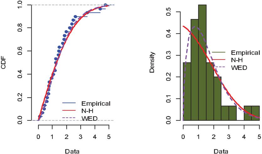
Figure 1 The empirical CDF vs the fitted CDF, the data histogram versus the fitted PDF.

Table 13 MLEs, K-S distances and p-values based on complete data

	Estimated Parameters
Distribution	$\alpha$	$\beta$	K-S Distance	p-Value
NH	4.4487206	0.0976619	0.11308	0.8377
Weibull	1.463405	2.192368	0.074834	0.996

Now, using SSPALT, we will analyse the supplied data by setting the value of $\tau$ to be 1.2 and $\eta$ to be 2.4. Now we take the total number of failures $m=20$ from a total of $n=30$ observations. To generate AT-II PHC data, we additionally assume the ${\xi }_i$ values as ${\xi }_1={\xi }_2=\mathrm{\cdots }={\xi }_8=0,{\xi }_9={\xi }_{10}=1$, ${\xi }_{11}=0,{\xi }_{12}=1,{\xi }_{13}=0,{\xi }_{14}={\xi }_{15}=1$, ${\xi }_{16}={\xi }_{17}={\xi }_{18}={\xi }_{19}=0$, ${\xi }_{20}=5$. As a result, failure data generated under normal and stress conditions from the real data given in Table 14 is as follows:

Table 14 The generated AT-II PHC data set

Normal Condition:	0.11	0.30	0.40	0.45	0.59	0.63	0.70	0.71	0.74	0.94	1.17
Stress Condition:	1.23	1.24	1.43	1.49	1.82	1.86	1.97	2.23	2.37

On the basis of the AT-II PHC data reported in Table 14, the parameters have been estimated for the NH distribution under the SSPALT model, and the obtained results are reported below in the Table 15:

Table 15 MLEs with MSEs under SSPALT for AT-II PHC data

Censoring	$\widehat{\alpha }$		$\widehat{\beta }$		$\widehat{\theta }$
AT-II PHCS	MLE	MSE	MLE	MSE	MLE	MSE
	1.512977	0.0057683	0.8767266	0.0032576	1.674958	0.028726

7 Discussion and Conclusion

In this article, the NH distribution is employed as a lifespan distribution for failures of objects put in SSPALT. AT-II PHCS was utilized to collect data from the experiment because of its flexibility in removing data from the experiment after it was started. In AT-II PHCS, whenever a failure happens, pre-specified objects from the experiment can be deleted. At each failure, the process is repeated until a targeted number of failures or the time limit for the experiment is reached. The MLE method was used to estimate the parameters, assuming that the influence of stress change in SSPALT is explained by a TRV model.

Thorough simulations have been conducted using R software to assess the efficacy of the suggested approach and statistical assumptions in this study. Tables 1–5 shows that the MSEs decrease for all increasing values of m, while all other variables, n, $\tau$, and $\eta$, remain constant. We can also see that when (n, m) increases, the values of MSEs and RABs decrease. When we increase the stress change time $\tau$, the MSEs and RABs get smaller, and we likewise receive reduced values of these estimates when we increase the censoring time $\eta$.

For estimated parameters, 95% ACIs were also obtained and are shown in Tables 6–10. Additionally, optimal test techniques based on the A and D optimality criteria were assessed. The FIM was likewise designed to provide the optimum value for its inverse. The A-optimality criterion reveals that this matrix has the least variance, which is nothing more than the inverse FIM trace. Table 11 depicts the optimal stress change timings. Finally, a real-world example based on the times between breakdowns for a repairable system was offered to better demonstrate the proposed technique, and the findings based on the real case were fairly promising. Therefore, it may be concluded that the model performs well enough to be considered for use in real-world studies where failures follow NH distribution patterns.

References

[1] Nadarajah, S., and Haghighi, F. (2011). An extension of the exponential distribution. Statistics, 45(6), 543–558.

[2] Mir Mostafaee, S. K., Asgharzadeh, A., and Fallah, A. (2016). Record values from NH distribution and associated inference. Metron, 74(1), 37–59.

[3] Sana, M. S., and Faizan, M. (2019). Bayesian Estimation for Nadarajah-Haghighi Distribution Based on Upper Record Values. Pak J Stat Oper Res, 15(1), 217–230.

[4] Selim, M.A. (2018). Estimation and prediction for Nadarajah-Haghighi distribution based on record values, Pak J Stat, 34(1), 77–90.

[5] Kamal, M., Alamri, O. A., and Ansari, S. I. (2020a). A new extension of the Nadarajah Haghighi model: mathematical properties and applications. Journal of Mathematical and Computational Science, 10(6), 2891–2906.

[6] MINIC, M. (2020). Estimation of parameters of Nadarajah-Haghighi extension of the exponential distribution using perfect and imperfect ranked set sample. Yugoslav Journal of Operations Research, 30(2), 177–198.

[7] Kamal, M., Rahman, A., Ansari, S. I., and Zarrin, S. (2020b). Statistical Analysis and Optimum Step Stress Accelerated Life Test Design for Nadarajah Haghighi Distribution. Reliability: Theory & Applications, 15(4), 1–9.

[8] Kamal, M., Zarrin, S., and Islam, A. (2013a). Accelerated life testing design using geometric process for Pareto distribution. Int. J. of Adv. Statistics and Probability, 1(2), 25–31.

[9] Rahman, A., Sindhu, T. N., Lone, S. A., and Kamal, M. (2020). Statistical inference for Burr Type X distribution using geometric process in accelerated life testing design for time censored data. Pakistan Journal of Statistics and Operation Research, 16(3), 577–586.

[10] Hakamipour, N. (2021). Comparison between constant-stress and step-stress accelerated life tests under a cost constraint for progressive type I censoring. Sequential Analysis, 40(1), 17–31.

[11] Zhang, X., Yang, J., and Kong, X. (2021). Planning constant-stress accelerated life tests with multiple stresses based on D-optimal design. Quality and Reliability Engineering International, 37(1), 60–77.

[12] Kamal, M. (2021). Parameter estimation for progressive censored data under accelerated life test with $k$ levels of constant stress. Reliability: Theory & Applications, 16(3), 149–159.

[13] Abd El-Raheem, A. M. (2021). Optimal design of multiple constant-stress accelerated life testing for the extension of the exponential distribution under type-II censoring. Journal of Computational and Applied Mathematics, 382, 113094.

[14] Saxena, S., Zarrin, S., Kamal, M., and Ul-Islam, A. (2012). Optimum step stress accelerated life testing for Rayleigh distribution. International Journal of Statistics and Applications, 2(6), 120–125.

[15] Kamal, M., Zarrin, S. and Islam, A. (2013b). Step stress accelerated life testing plan for two parameter Pareto distribution. Reliability: Theory & Applications, 8(1), 30–40.

[16] Hakamipour, N. (2020). Approximated optimal design for a bivariate step-stress accelerated life test with generalized exponential distribution under type-I progressive censoring. International Journal of Quality & Reliability Management, 38(5), 1090–1115. https://doi.org/10.1108/IJQRM-05-2020-0150

[17] Khan, M. A., and Chandra, N. (2021). Optimal Plan and Estimation for Bivariate Step-Stress Accelerated Life Test under Progressive Type-I Censoring. Pakistan Journal of Statistics and Operation Research, 17(3), 683–694.

[18] Amleh, M. A., and Raqab, M. Z. (2021). Inference in Simple Step-Stress Accelerated Life Tests for Type-II Censoring Lomax Data. Journal of Statistical Theory and Applications, 20(2), 364–379.

[19] Zarrin, S., Kamal, M., and Saxena, S. (2012). Estimation in constant stress partially accelerated life tests for Rayleigh distribution using type-I censoring. Reliability: Theory & Applications, 7(4), 41–52.

[20] Kamal, M., Zarrin, S., and Islam, A. U. (2013c). Constant stress partially accelerated life test design for inverted Weibull distribution with type-I censoring. Algorithms Research, 2(2), 43–49.

[21] Hassan, A. S., Nassr, S. G., Pramanik, S., and Maiti, S. S. (2020). Estimation in constant stress partially accelerated life tests for Weibull distribution based on censored competing risks data. Annals of Data Science, 7(1), 45–62.

[22] Rabie, A. (2021). E-Bayesian estimation for a constant-stress partially accelerated life test based on Burr-X Type-I hybrid censored data. Journal of Statistics and Management Systems, 1–19.

[23] Goel, P. K. (1971). Some estimation problems in the study of tampered random variables. (Ph.D. Thesis), Department of Statistics, Cranegie-Mellon University, Pittsburgh, Pennsylvania.

[24] DeGroot, M. H., and Goel, P. K. (1979). Bayesian estimation and optimal designs in partially accelerated life testing. Nav Res Logist, 26(2), 223–235.

[25] Bai, D. S., and Chung, S. W. (1992). Optimal design of partially accelerated life tests for the exponential distribution under type-I censoring. IEEE Trans Reliab, 41(3), 400–406.

[26] Bai, D. S., Chung, S. W., and Chun, Y. R. (1993a). Optimal design of partially accelerated life tests for the lognormal distribution under type I censoring. Reliab Eng Syst Saf, 40(1), 85–92.

[27] Rahman, A., Lone, S. A., and Islam, A. (2016). Parameter Estimation of Mukherjee-Islam Model under Step Stress Partially Accelerated Life Tests with Failure Constraint. Reliability: Theory & Applications, 11(4).

[28] Rahman, A., Lone, S. A., and Islam, A. (2019). Analysis of exponentiated exponential model under step stress partially accelerated life testing plan using progressive type-II censored data. Investigación Operacional, 39(4), 551–559.

[29] Epstein, B. (1954). Truncated life tests in the exponential case. Ann Math Stat, 555–564.

[30] Banerjee, A., and Kundu, D. (2008). Inference based on type-II hybrid censored data from a Weibull distribution. IEEE Trans Reliab, 57(2), 369–378.

[31] Balakrishnan, N., and Kundu, D. (2013). Hybrid censoring: Models, inferential results and applications. Comput Stat Data Anal, 57(1), 166–209.

[32] Balakrishnan, N. (2007). Progressive censoring methodology: an appraisal. Test, 16(2), 211–296.

[33] Balakrishnan, N., and Cramer, E. (2014). The art of progressive censoring: applications to reliability and quality, Statistics for industry and technology, Springer Link.

[34] Kundu, D., and Joarder, A. (2006). Analysis of Type-II progressively hybrid censored data. Comput Stat Data Anal, 50(10), 2509–2528.

[35] Ng, H. K. T., Kundu, D., and Chan, P. S. (2009). Statistical analysis of exponential lifetimes under an adaptive Type-II progressive censoring scheme. Nav Res Logist (NRL), 56(8), 687–698.

[36] Lin, C. T., Ng, H. K. T., and Chan, P. S. (2009). Statistical inference of Type-II progressively hybrid censored data with Weibull lifetimes. Comm Stat Theor Meth, 38(10), 1710–1729.

[37] Hemmati, F., and Khorram, E. (2013). Statistical analysis of the log-normal distribution under type-II progressive hybrid censoring schemes. Comm Stat Simulat Comput, 42(1), 52–75.

[38] Ismail, A. A. (2014). Inference for a step-stress partially accelerated life test model with an adaptive Type-II progressively hybrid censored data from Weibull distribution. J Comput Appl Math, 260, 533–542.

[39] Sobhi, M. M. A., and Soliman, A. A. (2016). Estimation for the exponentiated Weibull model with adaptive Type-II progressive censored schemes. Appl Math Model, 40(2), 1180–1192.

[40] Zhang, C., and Shi, Y. (2016). Estimation of the extended Weibull parameters and acceleration factors in the step-stress accelerated life tests under an adaptive progressively hybrid censoring data. J Stat Comput Simulat, 86(16), 3303–3314.

[41] Nassar, M., Nassr, S. G., and Dey, S. (2017). Analysis of burr Type-XII distribution under step stress partially accelerated life tests with Type-I and adaptive Type-II progressively hybrid censoring schemes. Ann Data Scien, 4(2), 227–248.

[42] Selim, M.A. (2018). Estimation and prediction for Nadarajah-Haghighi distribution based on record values, Pak J Stat, 34(1), 77–90.

[43] Alam, I., and Ahmed, A. (2020). Parametric and Interval Estimation Under Step-Stress Partially Accelerated Life Tests Using Adaptive Type-II Progressive Hybrid Censoring. Annl Dat Scien, 1–13. https://doi.org/10.1007/s40745-020-00249-1

[44] Murthy, D. P., Xie, M., and Jiang, R. (2004). Weibull models (Vol. 505). John Wiley and Sons, Inc., Hoboken, New Jersey.

Biographies

Mustafa Kamal is an Assistant Professor at Saudi Electronic University’s College of Science and Theoretical Studies. In 2013, he received his Ph.D. (Statistics) from Aligarh Muslim University, India. He authored more than 20 research papers that have been published in a variety of international journals. His main research interests include Accelerated Life testing & Reliability theory. Currently he is working on Bayesian estimation, Artificial intelligence and neural networks techniques, Sustainable Energy, Survey Sampling; Order Statistics; Statistical Inference and Distribution Theory.

Ahmadur Rahman is working as Assistant Professor in the department of Statistics and Operations Research, Aligarh Muslim University, Aligarh. He received his Bachelor, Master and PhD degree from Aligarh Muslim University in Statistics. He has published several research papers in national and international reputed journals. His areas of research are Life Testing, Accelerated Life Testing Plans, Reliability Analysis, Survival Analysis, Bayesian inference and Econometrics with R language/software.

Shazia Zarrin earned her Ph.D. in “Statistics” from the Department of Statistics and Operations Research, Aligarh Muslim University, India. Her primary research interests are in reliability theory and accelerated life testing. She is currently working on the Bayesian estimation technique in life testing and reliability estimation and applying computational techniques to field reliability and survival data using R software. She is an active reviewer for a number of prestigious international journals.

Haneefa Kausar earned her Ph.D. in “Operations Research” from the Department of Statistics and Operations Research, Aligarh Muslim University, Aligarh, India. Her area of research is Mathematical Programming, Bi-level Programming, Multi-level Programming, Linear Fractional Programming, Non Linear Fractional Programming and Accelerated Life Testing plan. She has published number of papers in very good journals.

Journal of Reliability and Statistical Studies, Vol. 14, Issue 2 (2021), 585–614.
doi: 10.13052/jrss0974-8024.14211
© 2021 River Publishers