Inverted Topp-Leone Distribution: Contribution to a Family of J-Shaped Frequency Functions in Presence of Random Censoring

Hiba Zeyada Muhammed^1,* and Essam Abd Elsalam Muhammed²

¹Department of Mathematical Statistics, Faculty of Graduate Studies for Statistical Research, Cairo University, Egypt

²Department of Management and Financial, High Institute of Computer and Information Technology, Elshorouk Academy, Egypt

E-mail: hiba_stat@cu.edu.eg; essamabdelsalam16@gmail.com

*Corresponding Author

Received 31 July 2021; Accepted 11 November 2021; Publication 06 December 2021

Abstract

In this paper, Bayesian and non-Bayesian estimation of the inverted Topp-Leone distribution shape parameter are studied when the sample is complete and random censored. The maximum likelihood estimator (MLE) and Bayes estimator of the unknown parameter are proposed. The Bayes estimates (BEs) have been computed based on the squared error loss (SEL) function and using Markov Chain Monte Carlo (MCMC) techniques. The asymptotic, bootstrap (p,t), and highest posterior density intervals are computed. The Metropolis Hasting algorithm is proposed for Bayes estimates. Monte Carlo simulation is performed to compare the performances of the proposed methods and one real data set has been analyzed for illustrative purposes.

Keywords: Inverted Topp leone distribution, moments, order statistic, maximum likelihood estimation, Bayesian estimation, MCMC, highest posterior density interval, asymptotic confidence interval, bootstrap confidence interval, random censoring.

1 Introduction

The Topp-Leone (TL) distribution was originally proposed by [1] as an alternative to beta distribution and it has applied for some family data. In recent years, the TL distribution has received huge attention in the literature; see for example; [2] showed that the TL distribution exhibits bathtub failure rate function with widespread applications in reliability. Moreover, [3] showed that TL distribution possesses some attractive reliability properties such as bath tub-shape hazard rate, decreasing reversed hazard rate, upside-down mean residual life, and increasing expected inactivity time. Recently, [4] derived admissible minimax estimates for the shape parameter of the TL distribution under squared and linear-exponential loss functions. Recently, [5] introduced the inverted Topp-Leone (IVT) distribution as a J-shaped distribution. Which is useful for modeling lifetime Phenomena and she studied more of its properties.

In this paper, we study classical and Bayesian estimation for the shape parameter of the IVT distribution when the sample is complete and random censored.

The random censoring can be expressed as follows: When the units under test lose or remove from the test before its failure this data is called random censoring. To more illustrate, in clinical trials or medical tests, some patients retreat or leave the test before finishing it.

The work in this paper is organized as follows: In Section 2 we introduce the IVT distribution. The maximum likelihood estimator (MLE) of the unknown parameter, the Bayes estimator, and the confidence interval based on complete data will be introduced in Section 3, in Section 4 we introduce the maximum likelihood estimators (MLEs) of the unknown parameters, the Bayes estimators and the confidence intervals based on random censoring data. Finally, the paper is concluded in Section 5.

2 Inverted Topp-Leone Distribution

The Topp Leone distribution is defined with the following pdf and cdf respectively,

$$F(t;\beta )=t^{\beta }{(2-t)}^{\beta }$$

(1)

And

$$f(t;\beta )=\beta (2-2t){(2t-t^2)}^{\beta -1}$$

(2)

For $0<t<1$ and $\beta >0.$

Assume $X=\frac{1}{T}$ the pdf and cdf of $X$ are given respectively, as

$$f(x;\beta )=2\beta (x-1)x^{-2\beta -1}{(2x-1)}^{\beta -1},$$

(3)

And

$$F(x;\beta )=1-x^{-2\beta }{(2x-1)}^{\beta }.$$

(4)

For $1<x<\mathrm{\infty }$ and $\beta >0.$

In this case, the distribution of X is called inverted Topp-Leone (IVT) distribution denoted by $(\beta )$. It can be showed that the pdf (3) satisfies the following generalized Pearson system of differential equation

$$\frac{\acute{f(x)}}{f(x)}=\frac{a_0+a_{1}x+a_2{x}^2}{b_0+b_{1}x+b_2{x}^2+b_3{x}^3}$$

where $a_0=-2\beta -2$, $a_1=6\beta$, $a_2=-2\beta -2$, $b_0=0$, $b_1=1$, $b_2=-3$ and $b_3=2$.

The IVT distribution may be considered as a J- shaped because $f(x)>0$, $\frac{df(x)}{dx}<0$ and for some values $\frac{d^{2}f(x)}{d{x}^2}>0$. And it can be noted that from Figure 1. Also, Figure 2 shows the cdf of IVT distribution for different values for the parameter $\beta$.

The mode of the $\mathit{IVT}(\beta )$ is given by $1+\sqrt{\frac{3}{2\beta +2}}.$

The quantiles of the $\mathit{IVT}(\beta )$ distribution is given by

$$x_q=q^{\frac{-1}{\beta }}\left(1+\sqrt{1-q^{\frac{1}{\beta }}}\right),\mathrm{\hspace{0.25em}0}<q<1.$$

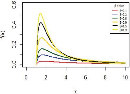
Figure 1 The pdf for IVT distribution.

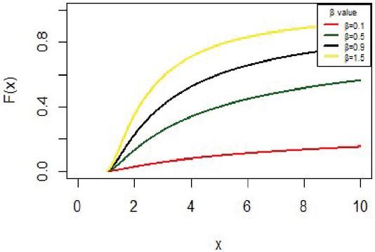
Figure 2 The cdf for IVT distribution.

The median is a special case from the quantile function, when $q=\frac{1}{2},$

$$x_{0.5}={(0.5)}^{\frac{-1}{\beta }}\left(1+\sqrt{1-{(0.5)}^{\frac{1}{\beta }}}\right)$$

And the inter-quartile range (IQR) is given as

$$\mathit{IQR}={\left(\frac{3}{4}\right)}^{\frac{-1}{\beta }}\left(1+\sqrt{1-{\left(\frac{3}{4}\right)}^{\frac{1}{\beta }}}\right)-{\left(\frac{1}{4}\right)}^{\frac{-1}{\beta }}\left(1+\sqrt{1-{\left(\frac{1}{4}\right)}^{\frac{1}{\beta }}}\right).$$

The $k^{th}$ moment about origin $\acute{{\mu }_k}$ is given by the following theorem.

Theorem 1: the $k^{th}$-moment about zero $\acute{{\mu }_k}$ $X$ is given by

$$\acute{{\mu }_k}=\beta \sum _{j=0}^{\mathrm{\infty }}\frac{c(k,j){(-1)}^j}{j-k+\beta }$$

(5)

For $k=1\mathrm{\dots }n$ and $\beta \ne 1$

Where

$c(k,0)$	$=2^k,c(k,1)=k{2}^{k-1}\mathit{\hspace{1em}}\text{and}$
$c(k,j)$	$={\displaystyle \frac{k{2}^{k-2j}}{j!}}{\displaystyle \prod _{i=1}^{j-1}}(k-j-i),j\ge 2.$

The survival function for the failure time X follows IVT distribution is defined as

$$R(x)=x^{-2\beta }{(2x-1)}^{\beta }$$

(6)

For fixed x means the probability of survival up to time x. Figure 3 shows the survival function for the IVT distribution with different parameter values.

Moreover, for the IVT distribution, the hazard function is easily obtained as

$$h(x)=2\beta \frac{x-1}{x(2x-1)}.$$

(7)

and it has different shapes according to the values of the parameter $\beta$ as shown in Figure 4.

The reversed hazard function for the IVT distribution is given as follows

$$r(x)=\frac{2\beta (x-1)x^{-2\beta -1}{(2x-1)}^{\beta -1}}{1-x^{-2\beta }{(2x-1)}^{\beta }}.$$

(8)

and it has different shapes as shown in Figure 5 according to to the variability in the parameter $\beta$.

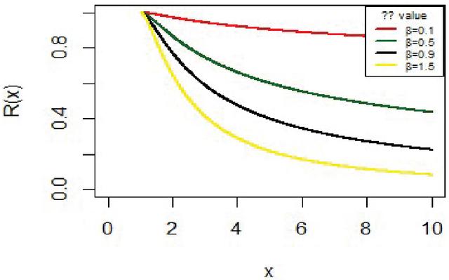
Figure 3 The reliability function for IVT distribution.

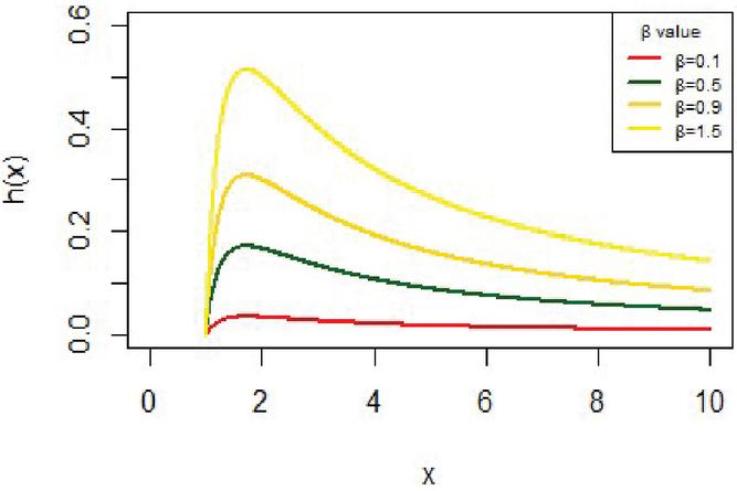
Figure 4 The hazard function for IVT distribution.

Figure 5 The reversed hazard function for IVT distribution.

2.1 Distributions and Moments of Order Statistics from IVT Distribution

Let $X_1,X_2,\mathrm{\dots },X_n$ be independent and identically distributed random variables drawn from IVT distribution. Let $X_{(r)};r=1,2,\mathrm{\dots },n,$ be the $r^{th}$ order statistic, then the pdf of $X_{(r)}$ is defined as

$$f_n(x)=C_{n,r}{[F(x)]}^{r-1}{[1-F(x)]}^{n-r}f(x)$$

Where $x=x_{(r)}$, and $C_{n,r}=\frac{n!}{r!(n-r)!}$.

$f_n(x)$	$=2\beta C_{n,r}(x-1)x^{2\beta (n-r-1)-1}{(2x-1)}^{\beta (n-r-1)-1}$
	$\mathrm{\hspace{1em}}\cdot {[1-x^{2\beta }{(2x-1)}^{\beta }]}^{\beta (n-r-1)-1}$

Special cases for $X_{(1)}$ and $X_{(n)}$ are respectively considered as

$$f_n(x)=2n\beta (x-1)x^{2\beta (n-2)-1}{(2x-1)}^{n\beta -1},x=x_{(1)}$$

and

$f_n(x)$	$=2n\beta (x-1)x^{-2\beta -1}{(2x-1)}^{\beta -1}{[1-x^{2\beta }{(2x-1)}^{\beta }]}^{n-1},$
$x$	$=x_{(n)}$

The joint pdf of $x_{(r)}$ and $x_{(s)}$, $1\le r<s\le n$, for a sample of size n

$f_n(x,y)$	$=C_{n,r,s}{[F(x)]}^{r-1}{[1-F(y)]}^{n-s}$
	$\mathrm{\hspace{1em}}\times {[F(y)-F(x)]}^{s-r-1}f(x)f(y)$

Where $x=x_{(r)},y=x_{(s)}$ and $C_{n,r,s}=\frac{n!}{r!(s-r-1)!(n-s)!}$.

$f_n(x,y)$	$=4{\beta }^2{C}_{n,r,s}{[1-x^{2\beta }{(2x-1)}^{\beta }]}^{r-1}{[y^{2\beta }{(2y-1)}^{\beta }]}^{n-s}$
	$\mathrm{\hspace{1em}}\cdot {[x^{2\beta }{(2x-1)}^{\beta }-y^{2\beta }{(2y-1)}^{\beta }]}^{s-r-1}$
	$\mathrm{\hspace{1em}}\cdot (x-1)x^{-2\beta -1}{(2x-1)}^{\beta -1}(y-1)y^{-2\beta -1}{(2y-1)}^{\beta -1},$
	$\mathrm{\hspace{1em}\hspace{1em}}1<x<y<\mathrm{\infty }$

In the following theorems, the moments and product moments about origin will be introduced

Theorem 2: the $k^{th}$-moment about zero ${\mu }_{r:n}^k$ of $r^{th}$ order statistic $X_{(r)}$ is given by

$${\mu }_{r:n}^k=C_{n,r}\sum _{j=0}^{\mathrm{\infty }}c(k,j){(-1)}^{\frac{1}{\beta }}B(\frac{j-k}{\beta }+1,n-r+1)$$

(9)

For $k=1\mathrm{\dots }n$ and $r=1\mathrm{\dots }n$,

Where

$c(k,0)$	$=2^k,c(k,1)=k{\mathrm{\hspace{0.25em}2}}^{k-1}\mathit{\hspace{1em}}\text{and}$
$c(k,j)$	$={\displaystyle \frac{k{\mathrm{\hspace{0.25em}2}}^{k-2j}}{j!}}{\displaystyle \prod _{i=1}^{j-1}}(k-j-i),j\ge 2,$

and $B(\cdot ,\cdot )$ is the beta function.

The $k^{th}$ moment of $X_{(1)}$ is given as

$${\mu }_{1:n}^k=n!\sum _{j=0}^{\mathrm{\infty }}c(k,j){(-1)}^{\frac{1}{\beta }}\frac{\mathrm{\Gamma }\left(\frac{j-k}{\beta }+1\right)}{\mathrm{\Gamma }\left(\frac{j-k}{\beta }+n+1\right)}.$$

The $k^{th}$ moment of $X_{(n)}$ is given as

$${\mu }_{n:n}^k=n\sum _{j=0}^{\mathrm{\infty }}c(k,j){(-1)}^{\frac{1}{\beta }}\frac{\mathrm{\Gamma }\left(\frac{j-k}{\beta }+n\right)}{\mathrm{\Gamma }\left(\frac{j-k}{\beta }+n+1\right)}.$$

Theorem 3: the $k^{th}$ and $L^{th}$-product moments about zero ${\mu }_{r:n}^{(k,L)}$ of $X_{(r)}$ and $X_{(s)}$ are given by

${\mu }_{r:n}^{(k,L)}$	$=C_{n,r,s}{\displaystyle \sum _{j_3}^{s-r-1}}{\displaystyle \sum _{j_2}^{\mathrm{\infty }}}{\displaystyle \sum _{j_1}^{\mathrm{\infty }}}c(k,j_1)c(L,j_2){\displaystyle \frac{\left(\genfrac{}{}{0.0pt}{}{s-r-1}{j_3}\right){(-1)}^{\frac{j_1+j_2}{\beta }+j_3}}{\frac{j_1-k}{\beta }+j_3+r}}$
	$\mathrm{\hspace{1em}}\cdot \mathit{B}({\displaystyle \frac{j_1+j_2-k-L}{\beta }}+s,n-s+1).$	(10)

For $k=1\mathrm{\dots }n$, $L=1\mathrm{\dots }n$ and $r=1\mathrm{\dots }n$.

Where $c(k,j_1),c(L,j_2)$ as given in (9).

3 Estimation Based on Complete Samples for IVT Distribution Shape Parameter

3.1 Maximum Likelihood Estimation

Suppose that $X_1,X_2,\mathrm{\dots },X_n$ is a simple random sample of size n drawn from $\mathrm{IVT}(\beta )$. In this section, the shape parameter of the IVT distribution will be estimated using the MLE as follows.

The likelihood function is given by

$$l(x;\beta )=\prod _{i=1}^{n}2\beta (x_i-1)x_i^{-(2\beta +1)}{(2x_i-1)}^{\beta -1}$$

(11)

The natural logarithm of the likelihood function is given as

$$L(x;\beta )\propto nlog(\beta )-(2\beta +1)\sum _{i=1}^n\log (x_i)+(\beta -1)\sum _{i=1}^n\log (2x_i-1)$$

After differentiating the $L(x;\beta )$ and equating to zero the MLE for $\beta$ can be expressed in closed form as follows

$$\widehat{\beta }=\frac{n}{{\sum }_{i=1}^n\log \mathrm{?}(x_i^2/(2x_i-1))}.$$

3.2 Bayesian Estimation

In this section, we have discussed the Bayesian estimation procedure for the parameter of the IVT distribution and we get the Bayesian estimate of the unknown parameter under the squared error loss (SEL) function. We assume that the unknown parameter of the IVT distribution have gamma prior distribution and can be written with proportional as follows;

$$\pi (\beta |{\mathrm{a}}_1,{\mathrm{b}}_1)\propto {\beta }^{{\mathrm{a}}_1-1}{\mathrm{e}}^{-\beta {\mathrm{b}}_1},\beta >0,{\mathrm{a}}_1,{\mathrm{b}}_1>0$$

(12)

Hyper-parameters determination: The hyper-parameters involved in priors (12) can be easily evaluated if we consider that prior mean and prior variance are known. The prior mean and prior variance will be obtained from the maximum likelihood estimate of $(\beta )$ by equating the mean and variance of $({\widehat{\beta }}^j)$ with the mean and variance of the considered priors (gamma prior), where $j=1,2,\mathrm{\dots },k$ and k is the number of random samples generated from the model in Section 3.1. Thus, on equating mean and variance of $({\widehat{\beta }}^j)$ with the mean and variance of gamma priors, we get ([6])

$$\frac{1}{k}\sum _{j=1}^k{\widehat{\beta }}^j=\frac{{\mathrm{a}}_1}{{\mathrm{b}}_1}\mathit{\hspace{1em}}\&\mathit{\hspace{1em}}\frac{1}{k-1}\sum _{j=1}^k{\left({\widehat{\beta }}^j-\frac{1}{k}\sum _{j=1}^k{\widehat{\beta }}^j\right)}^2=\frac{{\mathrm{a}}_1}{\mathrm{b}_1{}^2}$$

Now, on solving the above two equations, the estimated hyper-parameters can be written as

${\mathrm{a}}_1$	$={\displaystyle \frac{{\left(\frac{1}{k}{\sum }_{j=1}^k{\widehat{\beta }}^j\right)}^2}{\frac{1}{k-1}{\sum }_{j=1}^k{\left({\widehat{\beta }}^j-\frac{1}{k}{\sum }_{j=1}^k{\widehat{\beta }}^j\right)}^2}}\mathit{\hspace{1em}}\&$
${\mathrm{b}}_1$	$={\displaystyle \frac{\frac{1}{k}{\sum }_{j=1}^k{\widehat{\beta }}^j}{\frac{1}{k-1}{\sum }_{j=1}^k{\left({\widehat{\beta }}^j-\frac{1}{k}{\sum }_{j=1}^k{\widehat{\beta }}^j\right)}^2}}$

Based on the likelihood function (11) and the gamma prior (12), the joint posterior density function of $\beta$ given the data can be written as

$$\pi (\beta |\underset{¯}{x})=\frac{\pi (\beta )L(\beta |\underset{¯}{x})}{{\int }_0^{\mathrm{\infty }}\pi (\beta )L(\beta |\underset{¯}{x})\mathit{d}\beta }.$$

Then, the joint posterior density function can be written as

$$\pi (\beta |\underset{¯}{x})=\frac{1}{k(\beta )}\prod _{i=1}^{n}2(x_i-1)x_i^{-(2\beta +1)}{(2x_i-1)}^{\beta -1}{\beta }^{{\mathrm{a}}_1}{\mathrm{e}}^{-\beta {\mathrm{b}}_1}$$

(13)

Where,

$$k(\beta )={\int }_0^{\mathrm{\infty }}\prod _{i=1}^{n}2(x_i-1)x_i^{-(2\beta +1)}{(2x_i-1)}^{\beta -1}{\beta }^{{\mathrm{a}}_1}{\mathrm{e}}^{-\beta {\mathrm{b}}_1}d\beta ,$$

Thus, the Bayes estimate of $\beta$ based on SEL function is given by

$\tilde{\beta }$	$=E(\beta |\underset{¯}{x})$
$\tilde{\beta }$	$={\displaystyle \frac{{\int }_0^{\mathrm{\infty }}\beta \pi (\beta )L(\beta |\underset{¯}{x})\mathit{d}\beta }{{\int }_0^{\mathrm{\infty }}\pi (\beta )L(\beta |\underset{¯}{x})\mathit{d}\beta }}$	(14)

It should be noted that the ratio of integral in (3.2) cannot be obtained in closed forms. So, we use the MCMC approximation method to generate samples from (13) and to calculate the BE of $\beta$ and also to construct associated HPD intervals.

Markov Chain Monte Carlo (MCMC) is considered to be a computer-driven sampling technique. It permits one to characterize a distribution without knowing all of the distribution mathematical properties by random sampling values out of the distribution ([7]). We use Metropolis Hasting (M-H) method with normal proposal distribution to generate random numbers from (13). Thus, we perform the following steps of the M-H algorithm to draw samples from the posterior density (13) and in turn compute the Bayes estimate of $\beta$ and construct the corresponding HPD intervals ([8]):

I. Set initial values ${\theta }^{(0)},$ M $=$ burn-in.

II. For i $=$1,…,N, repeat the following steps.

∙ Set $\theta ={\theta }^{(i-1)}$.

∙ Generate new candidate parameter values $\omega$ from $N_1(\log (\theta ),S_{\theta }).$

∙ Set ${\theta }^{\prime }=\exp (\omega )$.

∙ Calculate $A=\min (1,\frac{\pi ({\theta }^{\prime }|\underset{¯}{\underset{¯}{x}})}{\pi (\theta |\underset{¯}{x})})$

∙ Update ${\theta }^{(i)}={\theta }^{\prime }$ with probability A; otherwise set ${\theta }^{(i)}=\theta .$

The approximate Bayes estimate of ${\theta }^{(i)}={({\beta }^{(i)})}^{\prime }$, $i=1,2,\mathrm{\dots }$,N with respect to SEL function is given by

$${\tilde{\theta }}_{BS}=\frac{1}{N-M}\sum _{i=M+1}^N{\theta }^{(i)},$$

Where ${\tilde{\theta }}_{\mathrm{BS}}$ is Bayes estimate under SEL function and M is the burn-in-period (that is, a number of iterations before the stationary distribution is achieved).

3.3 Interval Estimation for IVT Distribution Shape Parameter

In this section, we propose different confidence intervals. One is based on the asymptotic distribution of $\beta$, two different bootstrap confidence intervals, and finally, HPD intervals.

The Asymptotic Confidence Interval

The second derivative for $L(x;\beta )$ is trivially obtained as

$$\frac{d^{2}L}{d{\beta }^2}=-\frac{n}{{\beta }^2}.$$

The observed Fisher information matrix is given by

$$I(\widehat{\beta })=-{\frac{d^{2}L}{d{\beta }^2}|}_{\beta =\widehat{\beta }}=\frac{n}{{\widehat{\beta }}^2}$$

The asymptotic variance of $\widehat{\beta }$ is

$$V(\widehat{\beta })=\frac{1}{I(\widehat{\beta })}=\frac{{\widehat{\beta }}^2}{n}.$$

The sampling distribution of $\frac{\widehat{\beta }-\beta }{\sqrt{V(\widehat{\beta })}}$ can be approximated by a standard normal distribution.

The large sample $(1-\alpha )100\%$ confidence interval for $\beta$ is given by

$$({\widehat{\beta }}_L,{\widehat{\beta }}_U)=\widehat{\beta }\mp Z_{\frac{\alpha }{2}}\sqrt{V(\widehat{\beta })}.$$

where $Z_{\frac{\alpha }{2}}$ is the standard normal random variable and $(1-\alpha )$ is the confidence coefficient.

Bootstrap Confidence Intervals

The bootstrap confidence intervals are approximate confidence intervals but in general are better approximate than standard intervals. A parametric bootstrap interval provides much more information about the population value of the quantity of interest than does a point estimate. The parametric bootstrap methods are of two types: –

(i) The percentile bootstrap method (Boot-p) was proposed by [9].

(ii) The Bootstrap-t method (Boot-t) was proposed by [10].

Percentile Bootstrap (Boot-P) Confidence Interval

The boot-p method is rather simple and constructs confidence intervals directly from the percentiles of the bootstrap distribution of the estimated parameters. It is given by the following steps:

I. A complete sample is generated from the original data $\mathrm{T}=(t_1,t_2\mathrm{\dots }{t}_n)$ and the MLE $\widehat{\theta }={(\widehat{\beta })}^{\prime }$ of the parameter $\theta ={(\beta )}^{\prime }$ is computed.

II. Again, an independent complete bootstrap sample ${\mathrm{T}}^{*}=(t_1{}^{*},t_2{}^{*}\mathrm{\dots }t_n{}^{*})$ is generated by using $\widehat{\theta }$.

III. Now, compute the bootstrap MLE ${\widehat{\theta }}^{*}$ of parameter $\theta$ based on ${\mathrm{T}}^{*}$, as in step-1.

IV. Repeat steps 2–3, B times representing B bootstrap MLE’s ${\widehat{\theta }}^{*}$’s based on B different bootstrap samples, i $=$ 1,2,… B.

V. Arrange all ${\widehat{\theta }}^{*}$’s in an ascending order to obtain the bootstrap sample i.e. $\widehat{\theta }^{*}{}_{(1)}\le \widehat{\theta }^{*}{}_{(2)}\le \mathrm{\dots }\le \widehat{\theta }^{*}{}_{(\mathrm{B})}$. An approximate $100(1-\omega )\%$ boot-p confidence interval for $\theta$ is obtained by $(\widehat{\theta }^{*}{}_{[(\frac{\omega }{2})\times B]},\widehat{\theta }^{*}{}_{[(1-\frac{\omega }{2})\times B]})$.

Where, $\frac{\omega }{2}$ is the quantity that helps to determine the bootstrap point.

Bootstrap-t (Boot-t) Confidence Intervals

The bootstrap-t confidence interval is given by the following steps:

I. Steps 1 and 2 of boot-p and boot-t methods are the same.

II. Compute the bootstrap-t statistic ${\mathrm{T}}^{*}=\frac{\widehat{\theta }^{*}{}_{\mathrm{b}}-\widehat{\theta }}{\sqrt{\mathrm{v}(\widehat{\theta }^{*}{}_{\mathrm{b}})}}$ for $\widehat{\theta }^{*}{}_{\mathrm{b}}$ where b $=$ 1, 2,…B.

III. To obtain a set of bootstrap statistics $\mathrm{T}^{*}{}_i;\mathrm{i}=1,2,\mathrm{\dots },\mathrm{B}$ repeat steps 2–3, B times.

IV. Let $\mathrm{T}^{*}{}_{(1)}\le \mathrm{T}^{*}{}_{(2)}\le \mathrm{\cdots }\le \mathrm{T}^{*}{}_{(\mathrm{B})}$ be the ordered values of $\mathrm{T}^{*}{}_{\mathrm{i}}$; $\mathrm{i}=1,2,\mathrm{\dots },\mathrm{B}$.

V. Now, the approximate $100(1-\omega )\%$ boot-t confidence interval for parameter $\theta$ is obtained by

$$(\widehat{\theta }-\widehat{T}^{*}{}_{[(1-\frac{\omega }{2})\times B]}\sqrt{v(\widehat{\theta })},\widehat{\theta }-\widehat{T}^{*}{}_{[(\frac{\omega }{2})\times B]}\sqrt{v(\widehat{\theta })})$$

Highest Posterior Density (HPD) Intervals

The HPD intervals for the unknown parameters can be constructed by using the following algorithm: let ${\theta }_{(1)},{\theta }_{(2)},\mathrm{\dots },{\theta }_{(n)}$ be the corresponding ordered MCMC sample, to construct the HPD interval, let ${\theta }_{(j)}$ be the j${}^{\mathrm{th}}$ smallest of $\{{\theta }_{(i)}\}$ and denote $D_{\mathrm{j}}(n)=({\theta }_{(j)},{\theta }_{(j+[(1-\phi )n])})$, where $0<\phi <1$ For $\mathrm{j}=1,2,\mathrm{\dots },\mathrm{n}-[(1-\phi )\mathrm{n}]$ be the HPD intervals then the best HPD interval that has the smallest interval width from $D_{\mathrm{j}}{(n)}^{,}s$. So, we can say $D_{{\mathrm{j}}^{*}}(n)=({\theta }_{({\mathrm{j}}^{*})},{\theta }_{({\mathrm{j}}^{*}+[(1-\phi )n])})$, be HPD interval for the unknown parameters have the smallest interval width among all $D_{{\mathrm{j}}^{*}}{(n)}^{\prime }$s. Where ${\mathrm{j}}^{*}$ is chosen so that

$${\theta }_{({\mathrm{j}}^{*}+[(1-\phi )n])}-{\theta }_{({\mathrm{j}}^{*})}=\underset{1\le j\le n-[(1-\phi )n]}{\min }({\theta }_{(\mathrm{j}+[(1-\phi )n])}-{\theta }_{(\mathrm{j})})$$

Where ${\theta }_{(j)}={\beta }_{(j)}$, and ${\theta }_{(i)}={\beta }_{(i)}$ then the HPD intervals for the unknown parameters can be constructed.

3.4 Simulation Study

A simulation study was carried to check the performance of the accuracy of point and interval estimates for several cases, for which estimate the one parameter of IVT distribution ($\beta$) for the number of replications $(m=1000)$, for different sample sizes (n) as $n=25$, 50, 80, 100 and different parameters values. All the computations are performed using statistical software R.

The simulations results for MLE are summarized in Tables 2, 3, 4, and 5 and obtained by the following steps:

i. Specify initial values for parameter ($\beta$) as (0.5), (0.8), (1.2) and (1.9).

ii. Specify the sample size n. as $n=25,50,80,100$.

iii. Generate n standard uniform variates i.e. $U\sim \mathit{Uniform}(0,1)$.

iv. Generated complete samples of size n from IVT ($\beta$) distribution by using the formula $x=U^{\frac{-1}{\beta }}(1+\sqrt{1-U^{\frac{1}{\beta }}})$

v. Obtain the maximum likelihood estimates (MLEs).

vi. Obtain the mean, bias, mean squared error (MSE), asymptotic and bootstrap confidence intervals (CI’s) for the unknown parameters, average interval lengths (AILs), and coverage probability (CP) for the different sample size.

vii. Repeat steps 1–5 1000 times.

And the simulation results for the Bayesian estimate are summarized in Tables 2, 3, 4, and 5 which are obtained by the following steps:

i. Step I, ii, iii, iv, and v of the MLE simulation are the same

ii. By using the M-H algorithm shown in Section 3.2 under the informative prior and the non-informative prior and repeat the chain N times (N $=$ 10000) to obtain MCMC samples.

∙ For informative prior, we compute the hyperparameters for all simulation cases as in Table 1.

∙ For non-informative prior (P-II) we assume that hyper-parameter values are $a_1=b_1=0$.

iii. Compute the approximate Bayes estimator of $\beta$ under SEL function is given by

$${\tilde{\beta }}_{\mathit{SEL}}=\frac{1}{N-M}\sum _{i=M+1}^N{\mathrm{g}}_{SEL}({\beta }^{(i)}),i=1,2,\mathrm{\dots },N.$$

Where M ($=$2000) is the burn-in-period (that is, a number of iterations before the stationary distribution is achieved).

Repeat step i–iii (1000) times to obtain the mean, bias, mean squared error (MSE), HPD intervals for the unknown parameters, average interval lengths (AILs), and coverage probability (CP) for the different sample sizes.

Table 1 The hyper parameters values under complete data

		Initial Values
Hyper-Parameters		${\beta }_0=0.5$	${\beta }_0=0.8$	${\beta }_0=1.2$	${\beta }_0=1.9$
30	a1	23.97	23.95	23.94	23.88
	b1	45.85	28.75	19.21	12.00
50	a1	48.92	48.93	48.99	48.97
	b1	95.59	59.47	40.02	25.21
80	a1	78.91	78.86	79.05	79.04
	b1	155.47	97.51	64.86	41.17
100	a1	98.90	98.97	99.06	98.90
	b1	195.76	123.19	82.52	51.58

Table 2 Average estimated values, MSEs, bias, asymptotic and bootstrap (t-p) CI intervals of MLEs and BEs of IVT distribution parameters under complete data

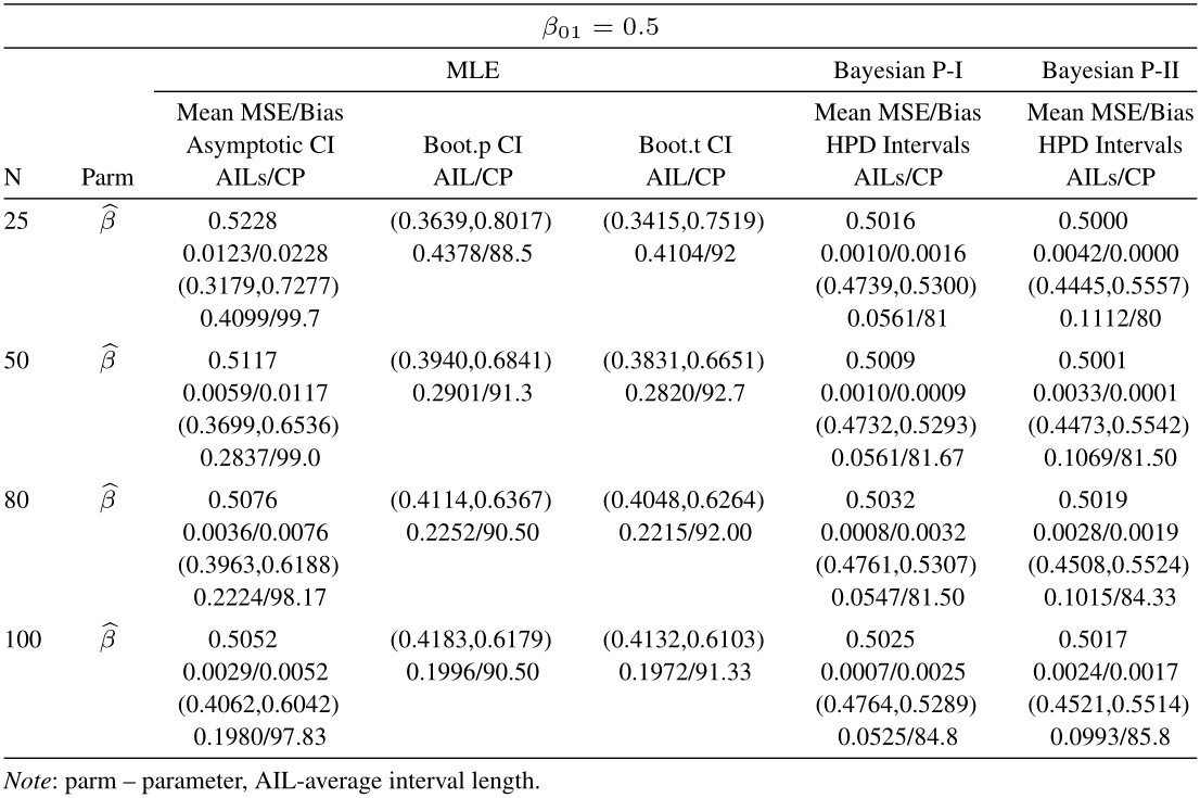
Table 3 Average estimated values, MSEs, bias, asymptotic and bootstrap (t-p) CI intervals of MLEs and BEs of IVT distribution parameters under complete data

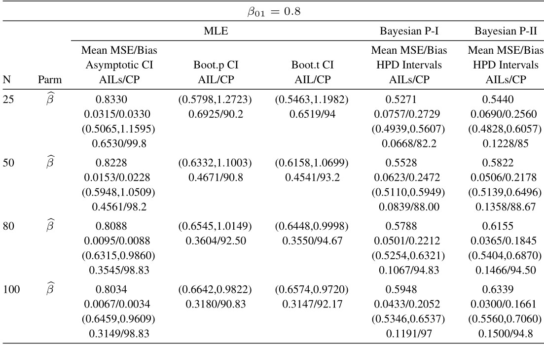
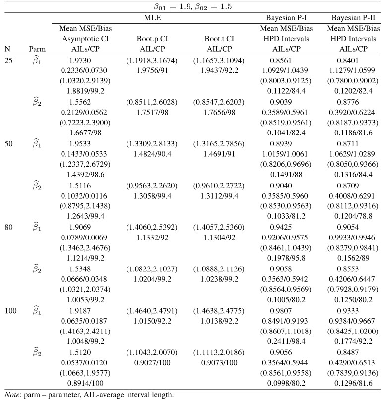
Table 4 Average estimated values, MSEs, bias, asymptotic and bootstrap (t-p) CI intervals of MLEs and BEs of IVT distribution parameters under complete data

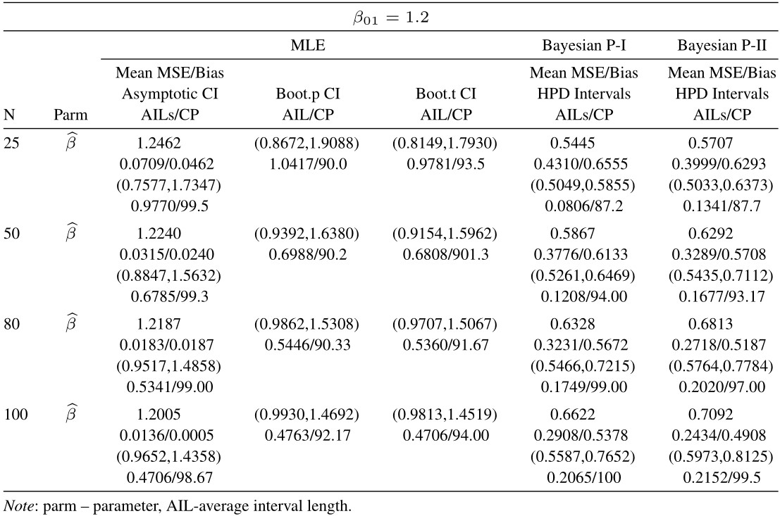
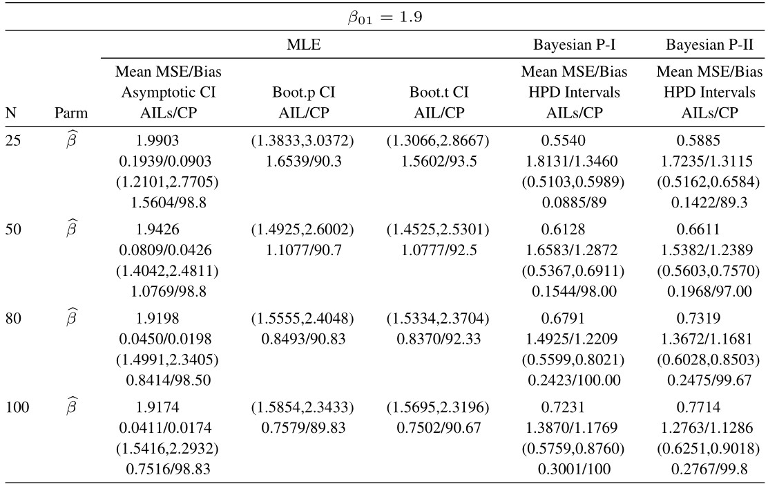
From tabulated values in Tables 2, 3, 4, and 5 it can be noticed that:

i. As expected, with respect to MSEs, higher values of n lead to better estimates.

ii. It is also noticed that the maximum likelihood estimates compete well with non-informative Bayes estimates, and the performance of the Bayes estimates obtained under informative prior is better than the non-informative Bayes estimates.

iii. It can also be noticed that under informative prior the AILs and associated CPs of HPD intervals are better than those of non-informative priors, bootstrap (p, t), and asymptotic confidence intervals respectively.

Table 5 Average estimated values, MSEs, bias, asymptotic and bootstrap (t-p) CI intervals of MLEs and BEs of IVT distribution parameters under complete data

3.5 Application to Real Data Set

In this section, the IVT distribution will be fitted to a real data set, to show how the IVT distribution can be applied in practice. moreover the IVT distribution will also compare with other inverted distributions that are fitted this data such as: inverse exponential (IE), inverse Rayleigh (IR), inverse Lindley(IL). And they will be introduced below as

The cdf, pdf of the inverse exponential (IE) distribution are respectively as

$$F_{IE}(x)=e^{-\frac{\lambda }{x}}\mathit{\hspace{1em}}x>0\mathit{\hspace{1em}}\mathrm{and}\mathit{\hspace{1em}}\lambda >0\mathit{\hspace{1em}}\mathrm{and}\mathit{\hspace{1em}}{f}_{IE}(x)=\frac{\lambda }{x^2}\mathit{\hspace{1em}}{e}^{-\frac{\lambda }{x}}.$$

The cdf, pdf of the inverse Rayleigh (IR) distribution are respectively as:

$F_{IR}(x)$	$=e^{-{(\frac{\sigma }{x})}^2}\mathit{\hspace{1em}}x>0\mathit{\hspace{1em}}\mathrm{and}\mathit{\hspace{1em}}\sigma >0\mathit{\hspace{1em}}\mathrm{and}$
$f_{IR}(x)$	$={\displaystyle \frac{2{\sigma }^2}{x^3}}{e}^{-{(\frac{\sigma }{x})}^2}.$

The cdf, pdf of the inverse Lindley (IL) distribution are respectively as

$F_{IL}(x)$	$=\left[1+{\displaystyle \frac{\theta }{1+\theta }}{\displaystyle \frac{1}{x}}\right]e^{-\frac{\theta }{x}}\mathit{\hspace{1em}}x>0\mathit{\hspace{1em}}\mathrm{and}\mathit{\hspace{1em}}\theta >0\mathit{\hspace{1em}}\mathrm{and}$
$f_{IL}(x)$	$={\displaystyle \frac{{\theta }^2}{1+\theta }}\left({\displaystyle \frac{1+x}{x^3}}\right)e^{-\frac{\theta }{x}}.$

The data set consists of 100 observations of breaking stress of carbon fibers in (Gba) which are listed as follows:
1.061, 1.117, 1.162, 1.183, 1.187, 1.192, 1.196, 1.213, 1.215, 1.219, 1.220, 1.224, 1.225, 1.228, 1.237, 1.240, 1.244, 1.259, 1.261, 1.263, 1.276, 1.310, 1.321, 1.329, 1.331, 1.337, 1.351, 1.359, 1.388, 1.408, 1.449, 1.449, 1.450, 1.459, 1.471, 1.475, 1.477, 1.480, 1.489, 1.501, 1.507, 1.515, 1.530,1.530, 1.533, 1.544, 1.544, 1.552, 1.556, 1.562, 1.566, 1.585, 1.586, 1.599, 1.602, 1.614, 1.616, 1.617, 1.628, 1.684, 1.711, 1.718, 1.733, 1.738, 1.743, 1.759, 1.777, 1.794, 1.799, 1.806, 1.814, 1.816, 1.828, 1.830, 1.884, 1.892, 1.944, 1.972, 1.984, 1.987, 2.020, 2.030, 2.029, 2.035, 2.037, 2.043, 2.046, 2.059, 2.111, 2.165, 2.686, 2.778, 2.972, 3.504, 3.863, 5.306

Figure 6 shows that the empirical date compared by the inverted distributions namely IVT, IE, IR and IL.

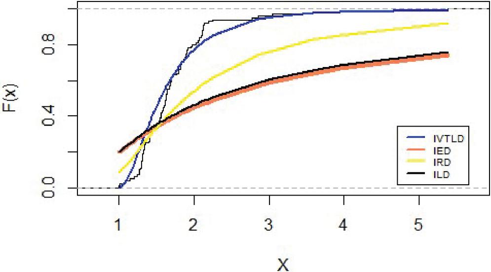
Figure 6 Empirical distribution for lifetimes for carbon fibers data.

Table 6 MLEs, AIC, BIC, AICC and HQIC values, and Kolmogorov-Smirnov statistics for carbon fibers data

		Measures
Model	MLE	p-value	K-S	-2log L	AIC	BIC	AICc	HQIC
IVT	5.6313	0.1197	0.1211	90.3201	92.3201	94.8844	90.3617	93.3566
IE	1.5680	0.0000	0.4528	290.4326	292.4326	294.9969	290.4742	293.4691
IR	1.5293	0.0000	0.3407	173.0542	175.0542	177.6185	173.0958	176.0907
IL	2.0773	0.0000	0.4350	280.3121	282.3121	284.8765	280.3538	283.3487

4 Estimation Based on Random Censored Samples for IVT Distribution Shape Parameter

4.1 Model Assumption and Description

The random censoring can be described as follows: if we have n units under test, Let their lifetime is ${\mathrm{T}}_1,{\mathrm{T}}_2,\mathrm{\dots },{\mathrm{T}}_{\mathrm{n}}$ which are independent and identically distributed (iid) random variables with pdf $f_T(t),t>0$ and cdf $F_T(t)t>0$, their random censoring times are $C_1,C_2,\mathrm{\dots },C_n$ which are iid with pdf $g_C(c),c>0$ and cdf $F_C(c),\mathrm{c}>0$, assume ${\mathrm{T}}_{\mathrm{i}}{}^{\prime }\mathrm{s}$ and ${\mathrm{C}}_{\mathrm{i}}{}^{\prime }\mathrm{s}$ be mutually independent. Note that, between ${\mathrm{T}}_{\mathrm{i}}{}^{\prime }\mathrm{s}$ and ${\mathrm{C}}_{\mathrm{i}}{}^{\prime }\mathrm{s}$, only one will be observed. Further, let the actual observed time be ${\mathrm{X}}_{\mathrm{i}}=\min ({\mathrm{T}}_{\mathrm{i}},{\mathrm{C}}_{\mathrm{i}}),\mathrm{i}=1,\mathrm{\dots },\mathrm{n}$, and the indicator variable ${\delta }_{\mathrm{i}}$ are defined as

$${\delta }_{\mathrm{i}}=\{\begin{array}{cc}1;\hfill & {\mathrm{T}}_{\mathrm{i}}\le {\mathrm{C}}_{\mathrm{i}}\hfill \\ 0;\hfill & {\mathrm{T}}_{\mathrm{i}}>{\mathrm{C}}_{\mathrm{i}}\hfill \end{array}$$

(15)

The censored data (${\mathrm{X}}_{\mathrm{i}}$) is known as the random censoring samples. The likelihood function under random censoring is given by [11]

$$L=\prod _{i=1}^n{[f_T(x)S_C(x_i)]}^{{\delta }_i}{[g_C(x_i)R_T(x_i)]}^{1-{\delta }_i}$$

(16)

Where, $R_T(x_i)=1-F_T(t)$ and $S_C(x_i)=1-F_C(c)$.

4.2 Maximum Likelihood Estimation

In this section, we obtain the MLEs for the unknown parameters of the IVT distribution. Let the lifetime T and censoring time C follow IVT $({\beta }_1)$ and IVT $({\beta }_2)$ respectively. Then the likelihood function for the unknown parameters under random censoring becomes:

$L$	$={\displaystyle \prod _{i=1}^n}{[2{\beta }_1(x_i-1)x_i{}^{-2{\beta }_1-2{\beta }_2-1}{(2x_i-1)}^{{\beta }_1+{\beta }_2-1}]}^{{\delta }_i}$
	$\mathrm{\hspace{1em}}{[2{\beta }_2(x_i-1)x^{-2{\beta }_2-2{\beta }_1-1}{(2x_i-1)}^{{\beta }_2+{\beta }_1-1}]}^{1-{\delta }_i}$	(17)

where ${\sum }_{i=1}^n{\delta }_i=\mathrm{r}$ is the observed number of uncensored lifetimes or failures.

Then, the corresponding log-likelihood function can be written as

$l$	$=rlog(2{\beta }_1)+{\displaystyle \sum _{i=1}^n}{\delta }_i\log (x_i-1)+(-2{\beta }_2-2{\beta }_1-1){\displaystyle \sum _{i=1}^n}{\delta }_i\log (x_i)$
	$\mathrm{\hspace{1em}}+({\beta }_1+{\beta }_2-1){\displaystyle \sum _{i=1}^n}{\delta }_i\log (2x_i-1)+(n-r)log(2{\beta }_2)$
	$\mathrm{\hspace{1em}}+{\displaystyle \sum _{i=1}^n}(1-{\delta }_i)\log (x_i-1)+(-2{\beta }_1-2{\beta }_2-1){\displaystyle \sum _{i=1}^n}(1-{\delta }_i)\log (x_i)$
	$\mathrm{\hspace{1em}}+({\beta }_2+{\beta }_1-1){\displaystyle \sum _{i=1}^n}(1-{\delta }_i)\log (2x_i-1)$	(18)

Differentiating (18) with respect to ${\beta }_1$ and ${\beta }_2$ gets:

${\displaystyle \frac{\partial l}{\partial {\beta }_1}}$	$={\displaystyle \frac{r}{{\beta }_1}}-2{\displaystyle \sum _{i=1}^n}{\delta }_i\log (x_i)+{\displaystyle \sum _{i=1}^n}{\delta }_i\log (2x_i-1)$
	$\mathrm{\hspace{1em}}-2{\displaystyle \sum _{i=1}^n}(1-{\delta }_i)\log (x_i)$
	$\mathrm{\hspace{1em}}+{\displaystyle \sum _{i=1}^n}(1-{\delta }_i)\log (2x_i-1)$	(19)
${\displaystyle \frac{\partial l}{\partial {\beta }_2}}$	$={\displaystyle \frac{n-r}{{\beta }_2}}-2{\displaystyle \sum _{i=1}^n}{\delta }_i\log (x_i)+{\displaystyle \sum _{i=1}^n}{\delta }_i\log (2x_i-1)$
	$\mathrm{\hspace{1em}}-2{\displaystyle \sum _{i=1}^n}(1-{\delta }_i)\log (x_i)$
	$\mathrm{\hspace{1em}}+{\displaystyle \sum _{i=1}^n}(1-{\delta }_i)\log (2x_i-1)$	(20)

Equating the first derivatives in (19) and (20) to zero and solving for ${\beta }_1$ and ${\beta }_2$ to get the MLEs ${\widehat{\beta }}_1$ and ${\widehat{\beta }}_2$ of ${\beta }_1$ and ${\beta }_2$, respectively in closed form as follows

$${\widehat{\beta }}_1=\frac{r}{\begin{array}{c}2{\sum }_{i=1}^n{\delta }_i\log (x)-{\sum }_{i=1}^n{\delta }_i\log (2x-1)\hfill \\ +2{\sum }_{i=1}^n(1-{\delta }_i)\log (x)-{\sum }_{i=1}^n(1-{\delta }_i)\log (2x-1)\hfill \end{array}}$$

and

$${\widehat{\beta }}_2=\frac{n-r}{\begin{array}{c}2{\sum }_{i=1}^n{\delta }_i\log (x)-{\sum }_{i=1}^n{\delta }_i\log (2x-1)\hfill \\ +2{\sum }_{i=1}^n(1-{\delta }_i)\log (x)-{\sum }_{i=1}^n(1-{\delta }_i)\log (2x-1)\hfill \end{array}}$$

4.3 Bayes Estimation for IVT Shape Parameter

In this section, we have discussed the Bayesian estimation procedure for the parameters of the IVT distribution based random censoring samples and we get BEs of the unknown parameters under the squared error loss (SEL) function. We assume that the unknown parameter of the IVT distribution has the independent gamma prior and can be written with proportional as follows;

$\pi ({\beta }_1|{\mathrm{a}}_1,{\mathrm{b}}_1)$	$\propto \beta _1{}^{{\mathrm{a}}_1-1}{\mathrm{e}}^{-{\beta }_1{\mathrm{b}}_1},{\beta }_1>0,{\mathrm{a}}_1,{\mathrm{b}}_1>0$	(21)
$\pi ({\beta }_2|{\mathrm{a}}_2,{\mathrm{b}}_2)$	$\propto \beta _2{}^{{\mathrm{a}}_2-1}{\mathrm{e}}^{-{\beta }_2{\mathrm{b}}_2},{\beta }_2>0,{\mathrm{a}}_2,{\mathrm{b}}_2>0$	(22)

Therefore, the joint prior density of ${\beta }_1$ and ${\beta }_2$ can be written with proportional as follows:

$$\pi ({\beta }_1,{\beta }_2)\propto \beta _1{}^{{\mathrm{a}}_1-1}\beta _2{}^{{\mathrm{a}}_2-1}{\mathrm{e}}^{-({\beta }_1{\mathrm{b}}_1+{\beta }_2{\mathrm{b}}_2)}{\beta }_1,{\beta }_2>0,{\mathrm{a}}_1,{\mathrm{a}}_2,{\mathrm{b}}_1,{\mathrm{b}}_2>0$$

(23)

Hyper-parameters determination: As in Section 3.2, the hyper-parameters involved in priors (21) and (22) can be easily evaluated, if we consider that prior mean and prior variance are known. The prior mean and prior variance will be obtained from the maximum likelihood estimates of $({\beta }_1,{\beta }_2)$ by equating the mean and variance of $(\widehat{\beta }_1{}^j,\widehat{\beta }_2{}^j)$ with the mean and variance of the considered priors (gamma prior), where $j=1,2,\mathrm{\dots },k$ and k is the number of random samples generated from the model in Section 4.2. Thus, on equating mean and variance of $(\widehat{\beta }_1{}^j,\widehat{\beta }_2{}^j)$ with the mean and variance of gamma priors, we get

$$\frac{1}{k}\sum _{j=1}^k\widehat{\beta }_1{}^j=\frac{{\mathrm{a}}_1}{{\mathrm{b}}_1}\mathit{\hspace{1em}}\&\mathit{\hspace{1em}}\frac{1}{k-1}\sum _{j=1}^k{(\widehat{\beta }_1{}^j-\frac{1}{k}\sum _{j=1}^k\widehat{\beta }_1{}^j)}^2=\frac{{\mathrm{a}}_1}{\mathrm{b}_1{}^2}$$

Now, on solving the above two equations, the estimated hyper-parameters can be written as

${\mathrm{a}}_1$	$={\displaystyle \frac{{\left(\frac{1}{k}{\sum }_{j=1}^k\widehat{\beta }_1{}^j\right)}^2}{\frac{1}{k-1}{\sum }_{j=1}^k{\left(\widehat{\beta }_1{}^j-\frac{1}{k}{\sum }_{j=1}^k\widehat{\beta }_1{}^j\right)}^2}}\mathit{\hspace{1em}}\&$
${\mathrm{b}}_1$	$={\displaystyle \frac{\frac{1}{k}{\sum }_{j=1}^k\widehat{\beta }_1{}^j}{\frac{1}{k-1}{\sum }_{j=1}^k{\left(\widehat{\beta }_1{}^j-\frac{1}{k}{\sum }_{j=1}^k\widehat{\beta }_1{}^j\right)}^2}}$

A similar procedure for determining the hyperparameters (${\mathrm{a}}_2,{\mathrm{b}}_2$) can be used for ${\beta }_2$.

Based on the likelihood function (4.2) and the joint prior density (23), the joint posterior density ${\beta }_1$ and ${\beta }_2$ given the data can be written as

$$\pi ({\beta }_1,{\beta }_2|\underset{¯}{x})=\frac{\pi ({\beta }_1,{\beta }_2)L({\beta }_1,{\beta }_2|\underset{¯}{x})}{{\int }_0^{\mathrm{\infty }}{\int }_0^{\mathrm{\infty }}\pi ({\beta }_1,{\beta }_2)L({\beta }_1,{\beta }_2|\underset{¯}{x})\mathit{d}{\beta }_1\mathit{d}{\beta }_2}.$$

Then, the joint posterior function can be written as

$\pi ({\beta }_1,{\beta }_2|\underset{¯}{x})$	$={\displaystyle \frac{1}{k({\beta }_1,{\beta }_2)}}4\beta _1{}^{r+{\mathrm{a}}_1-1}\beta _2{}^{(n-r)+{\mathrm{a}}_2-1}{\mathrm{e}}^{-({\beta }_1{\mathrm{b}}_1+{\beta }_2{\mathrm{b}}_2)}$
	$\mathrm{\hspace{1em}}{\displaystyle \prod _{i=1}^n}{(x_i-1)}^{{\delta }_i}{\displaystyle \prod _{i=1}^n}{(x_i-1)}^{1-{\delta }_i}$
	$\mathrm{\hspace{1em}}{\displaystyle \prod _{i=1}^n}x_i{}^{(-2{\beta }_1-2{\beta }_2-1){\delta }_i}{\displaystyle \prod _{i=1}^n}x_i{}^{(-2{\beta }_2-2{\beta }_1-1)(1-{\delta }_i)}$
	$\mathrm{\hspace{1em}}{\displaystyle \prod _{i=1}^n}{(2x_i-1)}^{({\beta }_2-{\beta }_1-1){\delta }_i}$
	$\mathrm{\hspace{1em}}{\displaystyle \prod _{i=1}^n}{(2x_i-1)}^{({\beta }_1-{\beta }_2-1)(1-{\delta }_i)}$	(24)

Where,

$k({\beta }_1,{\beta }_2)$	$={\displaystyle {\int }_0^{\mathrm{\infty }}}{\displaystyle {\int }_0^{\mathrm{\infty }}}4\beta _1{}^{r+{\mathrm{a}}_1-1}\beta _2{}^{(n-r)+{\mathrm{a}}_2-1}{\mathrm{e}}^{-({\beta }_1{\mathrm{b}}_1+{\beta }_2{\mathrm{b}}_2)}$
	$\mathrm{\hspace{1em}}\cdot {\displaystyle \prod _{i=1}^n}{(x_i-1)}^{{\delta }_i}\cdot {\displaystyle \prod _{i=1}^n}{(x_i-1)}^{1-{\delta }_i}$
	$\mathrm{\hspace{1em}}\cdot {\displaystyle \prod _{i=1}^n}x_i{}^{(-2{\beta }_1-2{\beta }_2-1){\delta }_i}{\displaystyle \prod _{i=1}^n}x_i{}^{(-2{\beta }_2-2{\beta }_1-1)(1-{\delta }_i)}$
	$\mathrm{\hspace{1em}}\cdot {\displaystyle \prod _{i=1}^n}{(2x_i-1)}^{({\beta }_2-{\beta }_1-1){\delta }_i}$
	$\mathrm{\hspace{1em}}\cdot {\displaystyle \prod _{i=1}^n}{(2x_i-1)}^{({\beta }_1-{\beta }_2-1)(1-{\delta }_i)}d{\beta }_1,d{\beta }_2,$

Thus, the Bayes estimate of $\mathrm{g}({\beta }_1,{\beta }_2)$ based on SEL function is given by

${\tilde{\mathrm{g}}}_{BS}({\beta }_1,{\beta }_2)$	$=E(\mathrm{g}({\beta }_1,{\beta }_2)|\underset{¯}{x})$
${\tilde{\mathrm{g}}}_{BS}({\beta }_1,{\beta }_2)$	$={\displaystyle \frac{{\int }_0^{\mathrm{\infty }}{\int }_0^{\mathrm{\infty }}\mathrm{g}({\beta }_1,{\beta }_2)\pi ({\beta }_1,{\beta }_2)L({\beta }_1,{\beta }_2|\underset{¯}{x})\mathit{d}{\beta }_1\mathit{d}{\beta }_2}{{\int }_0^{\mathrm{\infty }}{\int }_0^{\mathrm{\infty }}\pi ({\beta }_1,{\beta }_2)L({\beta }_1,{\beta }_2|\underset{¯}{x})\mathit{d}{\beta }_1\mathit{d}{\beta }_2}}$ (25)

It should be noted that the ratio of integral in (4.3) cannot be obtained in closed forms. So, we use the MCMC approximation method to generate samples from (24) and to calculate the BEs of ${\beta }_1$ and ${\beta }_2$ and also to construct associated HPD intervals. where we use the M-H method with normal proposal distribution.

4.4 Interval Estimation Based on Random Censoring Samples

In this section, we propose different confidence intervals. One is based on the asymptotic distribution of ${\beta }_1$ and ${\beta }_2$, two different bootstrap confidence intervals and finally, HPD intervals.

Asymptotic Confidence Intervals

The asymptotic variance-covariance matrix of the MLEs of ${\beta }_1$ and${\beta }_2$ can be obtained by inverting the observed information matrix, and is given as follows:

${\left[\begin{array}{cc}-E\left({\displaystyle \frac{{\partial }^2\mathrm{\ell }}{\partial \beta _1{}^2}}\right)\mathit{\hspace{1em}}\hfill & -E\left({\displaystyle \frac{{\partial }^2\mathrm{\ell }}{\partial {\beta }_1\partial {\beta }_2}}\right)\hfill \\ -E\left({\displaystyle \frac{{\partial }^2\mathrm{\ell }}{\partial {\beta }_2\partial {\beta }_1}}\right)\mathit{\hspace{1em}}\hfill & -E\left({\displaystyle \frac{{\partial }^2\mathrm{\ell }}{\partial \beta _2{}^2}}\right)\hfill \end{array}\right]}_{(\theta =\widehat{\theta })}^{-1}$

$\mathrm{\hspace{1em}\hspace{1em}}=\left[\begin{array}{cc}{V}_{11}\mathit{\hspace{1em}}\hfill & V_{12}\hfill \\ V_{21}\mathit{\hspace{1em}}\hfill & V_{22}\hfill \end{array}\right]$

Where $\widehat{\theta }={({\widehat{\beta }}_1,{\widehat{\beta }}_2)}^{\prime }$ and $\theta ={({\beta }_1,{\beta }_2)}^{\prime }$. The elements of the observed information matrix for ${\beta }_1$ and ${\beta }_2$ are given as follows:

$${\frac{{\partial }^{2}l}{\partial \beta _1{}^2}|}_{\theta =\widehat{\theta }}=-\frac{r}{\widehat{\beta }_1{}^2}$$

Then the observed fisher information

$$I({\widehat{\beta }}_1)=-{\frac{{\partial }^{2}l}{\partial \beta _1{}^2}|}_{\theta =\widehat{\theta }}=\frac{r}{\widehat{\beta }_1{}^2}$$

The asymptotic variance of ${\widehat{\beta }}_1$ is

$$V({\widehat{\beta }}_1)=\frac{1}{I({\widehat{\beta }}_1)}=\frac{\widehat{\beta }_1{}^2}{r}$$

and

$${\frac{{\partial }^{2}l}{\partial \beta _2{}^2}|}_{\theta =\widehat{\theta }}=-\frac{(n-r)}{\beta _2{}^2}$$

$$I({\widehat{\beta }}_1)=-{\frac{{\partial }^{2}l}{\partial \beta _2{}^2}|}_{\theta =\widehat{\theta }}=\frac{n-r}{\widehat{\beta }_2{}^2}$$

The asymptotic variance of ${\widehat{\beta }}_2$ is

$$V({\widehat{\beta }}_2)=\frac{1}{I({\widehat{\beta }}_2)}=\frac{\widehat{\beta }_2{}^2}{n-r}$$

The sampling distribution of $\frac{{\widehat{\beta }}_i-{\beta }_i}{\sqrt{v({\widehat{\beta }}_i)}}$ where $i=1,2$, can be approximated by a standard normal distribution. The large $(1-\alpha )100\%$ confidence intervals for ${\beta }_1$ and ${\beta }_2$ are given by

$$({\widehat{\beta }}_{iL},{\widehat{\beta }}_{iU})={\widehat{\beta }}_i\pm Z_{\frac{\alpha }{2}}\sqrt{v({\widehat{\beta }}_i)}\mathit{\hspace{1em}}\text{where}i=1,2.$$

Bootstrap Confidence Intervals

As in Section 3.3, two types of parametric bootstrap methods are considered

(iii) Percentile bootstrap method (Boot-p)

(iv) Bootstrap-t method (Boot-t)

Percentile Bootstrap (Boot-P) Confidence Interval

It given by the following steps:

i. A randomly censored sample is generated from the original data $\mathrm{T}=({\mathrm{t}}_1,{\mathrm{t}}_2\mathrm{\dots }{\mathrm{t}}_{\mathrm{n}})$ and the MLE $\widehat{\theta }=({\widehat{\beta }}_1$, ${\widehat{\beta }}_2){}^{\prime }$ of the parameter $\theta ={({\beta }_1,{\beta }_2)}^{\prime }$ is computed.

ii. Again, an independent randomly censored bootstrap sample ${\mathrm{T}}^{*}=(\mathrm{t}_1{}^{*},\mathrm{t}_2{}^{*}\mathrm{\dots }\mathrm{t}_{\mathrm{n}}{}^{*})$ is generated by using $\widehat{\theta }$.

iii. Now, compute the bootstrap MLE ${\widehat{\theta }}^{*}$ of parameter $\theta$ based on ${\mathrm{T}}^{*}$, as in step-1.

iv. Repeat steps 2–3, B times representing B bootstrap MLE’s ${\widehat{\theta }}^{*}$’s based on B different bootstrap samples, i $=$ 1,2,… B.

v. Arrange all ${\widehat{\theta }}^{*}$’s in an ascending order to obtain the bootstrap sample i.e. $\widehat{\theta }^{*}{}_{(1)}\le \widehat{\theta }^{*}{}_{(2)}\le \mathrm{\cdots }\le \widehat{\theta }^{*}{}_{(\mathrm{B})}$. An approximate $100(1-\omega )\%$ boot-p confidence interval for $\theta$ is obtained by $(\widehat{\theta }^{*}{}_{[(\frac{\omega }{2})\times B]},\widehat{\theta }^{*}{}_{[(1-\frac{\omega }{2})\times B]})$.

Where, $\frac{\omega }{2}$ is the quantity that helps to determine the bootstrap point.

Bootstrap-t (Boot-t) Confidence Intervals

The bootstrap-t confidence interval is given by the following steps:

i. Steps 1 and 2 of boot-p and boot-t methods are the same.

ii. Compute the bootstrap-t statistic ${\mathrm{T}}^{*}=\frac{\widehat{\theta }^{*}{}_{\mathrm{b}}-\widehat{\theta }}{\sqrt{\mathrm{v}(\widehat{\theta }^{*}{}_{\mathrm{b}})}}$ for $\widehat{\theta }^{*}{}_{\mathrm{b}}$ where b $=$ 1, 2,… B.

iii. To obtain a set of bootstrap statistics $\mathrm{T}^{*}{}_i;\mathrm{i}=1,2,\mathrm{\dots },\mathrm{B}$ repeat steps 2–3, B times.

iv. Let $\mathrm{T}^{*}{}_{(1)}\le \mathrm{T}^{*}{}_{(2)}\le \mathrm{\cdots }\le \mathrm{T}^{*}{}_{(\mathrm{B})}$ be the ordered values of $\mathrm{T}^{*}{}_{\mathrm{i}};\mathrm{i}=1,2,\mathrm{\dots },\mathrm{B}$.

v. Now, the approximate $100(1-\omega )\%$ boot-t confidence interval for parameter $\theta$ is obtained by

$$(\widehat{\theta }-\widehat{T}^{*}{}_{\left[\left(1-\frac{\omega }{2}\right)\times B\right]}\sqrt{v(\widehat{\theta })},\widehat{\theta }-\widehat{T}^{*}{}_{\left[\left(\frac{\omega }{2}\right)\times B\right]}\sqrt{v(\widehat{\theta })})$$

Highest Posterior Density (HPD) Intervals

As in Section 3.3, the HPD intervals for the unknown parameters can be constructed. let ${\theta }_{(1)},{\theta }_{(2)},\mathrm{\dots },{\theta }_{(n)}$ be the corresponding ordered MCMC sample, to construct the HPD interval, let ${\theta }_{(j)}$ be the j${}^{\mathrm{th}}$ smallest of $\{{\theta }_{(i)}\}$ and denote $D_{\mathrm{j}}(n)=({\theta }_{(j)},{\theta }_{(j+[(1-\phi )n])})$, where $0<\phi <1$. For $j=1,2,\mathrm{\dots },n-[(1-\phi )n]$ be the HPD intervals then the best HPD interval that has the smallest interval width from $D_{\mathrm{j}}(n)$’s. So, we can say $D_{{\mathrm{j}}^{*}}(n)=({\theta }_{({\mathrm{j}}^{*})},{\theta }_{({\mathrm{j}}^{*}+[(1-\phi )n])})$, be HPD interval for the unknown parameters have the smallest interval width among all $D_{{\mathrm{j}}^{*}}(n)$’s. Where ${\mathrm{j}}^{*}$ is chosen so that

$${\theta }_{({\mathrm{j}}^{*}+[(1-\phi )n])}-{\theta }_{({\mathrm{j}}^{*})}=\underset{1\le j\le n-[(1-\phi )n]}{\min }({\theta }_{(\mathrm{j}+[(1-\phi )n])}-{\theta }_{(\mathrm{j})})$$

Where ${\theta }_{(j)}={\beta }_{1(j)},{\beta }_{2(j)}$, and ${\theta }_{(i)}={\beta }_{1(i)},{\beta }_{2(i)}$ then the HPD intervals for the unknown parameters can be constructed.

4.5 Simulation Study

A simulation study was carried to check the performance of the accuracy of point and interval estimates for several cases, for which estimate the two parameters of IVT distribution (${\beta }_1$ and ${\beta }_2$) for number of replications $(m=1000)$, for different sample sizes (n) as $n=25$, 50, 80, 100 and different parameters values. All the computations are performed using statistical software R.

The simulations results for MLEs are summarized in Tables 8, 9, 10, and 11 and obtained by the following steps:

i. Specify initial values for parameters (${\beta }_1$ and ${\beta }_2$) as (0.5, 0.3), (0.8, 0.9), (1.2, 1) and (1.9, 1.5).

ii. Specify the sample size n. as $n=25,50,80,100.$

iii. Generate n standard uniform variates i.e. $U\sim \mathit{Uniform}(0,1)$.

iv. Generated samples of size n from IVT (${\beta }_1$) distribution (lifetimes) and IVT $({\beta }_2)$ (censoring times) distribution by using the formula

$t$	$=U^{\frac{-1}{{\beta }_1}}\left(1+\sqrt{1-U^{\frac{1}{{\beta }_1}}}\right)\mathit{\hspace{1em}}\text{and}$
$c$	$=U^{\frac{-1}{{\beta }_2}}\left(1+\sqrt{1-U^{\frac{1}{{\beta }_2}}}\right),\text{respectively}.$

v. Calculate the times $x_i=\min (T_i,C_i)$ and the censorship indicators ${\delta }_{\mathrm{i}}$, which are equal to 1 if $T_i<C_i$ and 0 otherwise.

vi. Obtain the maximum likelihood estimates (MLEs).

vii. Obtain the mean, bias, mean squared error (MSE), asymptotic and bootstrap confidence intervals (CI’s) for the unknown parameters, average interval lengths (AILs), and coverage probability (CP) for the different sample size.

viii. Repeat steps 1–5 1000 times.

And the simulation results for Bayesian estimates are summarized in Tables 8, 9, 10, and 11 which are obtained by the following steps:

iv. Step I, ii, iii, iv, and v of the MLEs simulation are the same

v. By using the M-H algorithm shown in Section 4.2 under the informative prior and the non-informative prior and repeat the chain N times (N $=$ 10000) to obtain MCMC samples.

∙ For informative prior, we compute the hyperparameters for all simulation cases as in Table 7.

∙ For non-informative prior (P-II) we assume that hyper-parameter values are $a_1=b_1=$ $a_2=b_2=a_3=$ $b_3=a_4=b_4=a_5=b_5=0$.

vi. Compute the approximate Bayes estimator of $\mathrm{g}({\beta }_1,{\beta }_2)$ under SEL is given by

$${\tilde{\mathrm{g}}}_{\mathit{SEL}}({\beta }_1,{\beta }_2)=\frac{1}{N-M}\sum _{i=M+1}^N{\mathrm{g}}_{\mathit{SEL}}(\beta _1{}^{(i)},\beta _2{}^{(i)},),i=1,2,\mathrm{\dots },N.$$

Where M ($=$2000) is the burn-in-period (that is, a number of iterations before the stationary distribution is achieved).

vii. Repeat step i–iii 1000 times to obtain the mean, bias, mean squared error (MSE), HPD intervals for the unknown parameters, average interval lengths (AILs), and coverage probability (CP) for the different sample size.

Table 7 The Hyper Parameters Values under random censoring data

		Initial Values
		${\beta }_{01}=0.5$,	${\beta }_{01}=0.8$,	${\beta }_{01}=1.2$,	${\beta }_{01}=1.9$,
Hyper-Parameters		${\beta }_{02}=0.3$	${\beta }_{02}=0.9$	${\beta }_{02}=1$	${\beta }_{02}=1.5$
30	a1	18.0	13.61	15.74	16.23
	a2	10.9	15.28	13.28	12.73
	b1	34.9	16.49	8.23	8.23
	b2	34.7	16.34	8.18	8.18
50	a1	30.7	22.81	22.81	27.64
	a2	18.3	26.12	26.12	21.41
	b1	60.2	27.87	14.15	14.15
	b2	60.2	27.86	14.17	14.17
80	a1	49.6	36.91	42.88	43.81
	a2	29.5	42.19	36.21	35.25
	b1	97.8	45.93	22.98	22.98
	b2	97.8	45.90	22.97	22.97
100	a1	61.3	46.57	54.36	55.37
	a2	37.7	52.37	44.60	43.60
	b1	121.7	57.66	28.86	28.86
	b2	121.7	57.61	28.84	28.84

Table 8 Average estimated values, MSEs, bias, asymptotic and bootstrap (t-p) CI intervals of MLEs and BEs of IVT distribution parameters under random censoring data

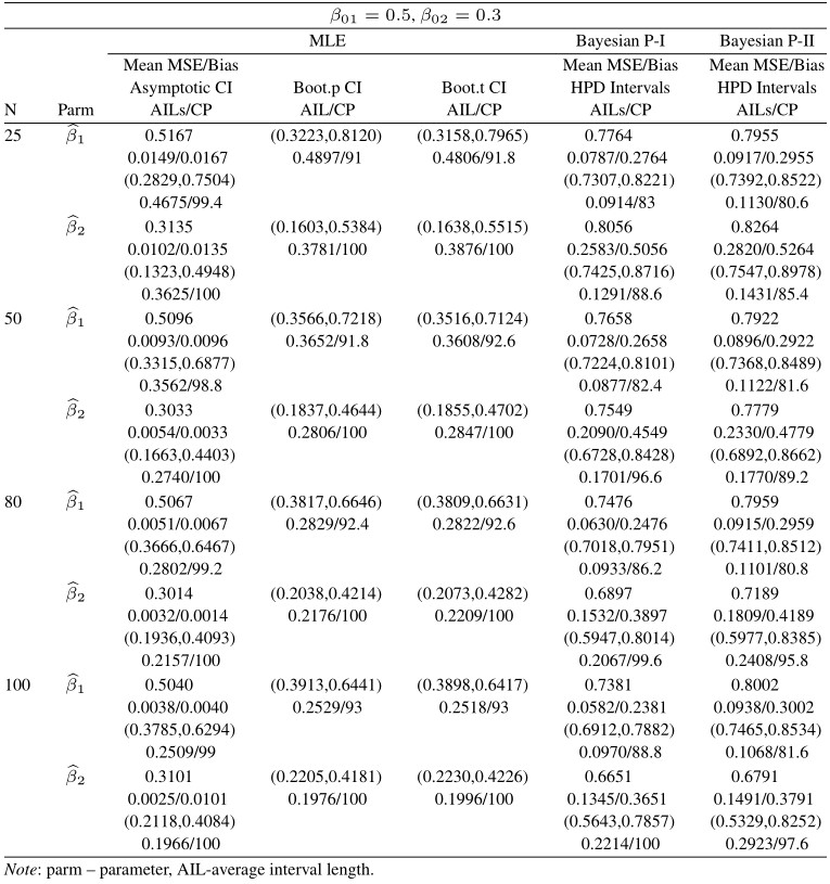
Table 9 Average estimated values, MSEs, bias, asymptotic and bootstrap (t-p) CI intervals of MLEs and BEs of IVT distribution parameters under random censoring data

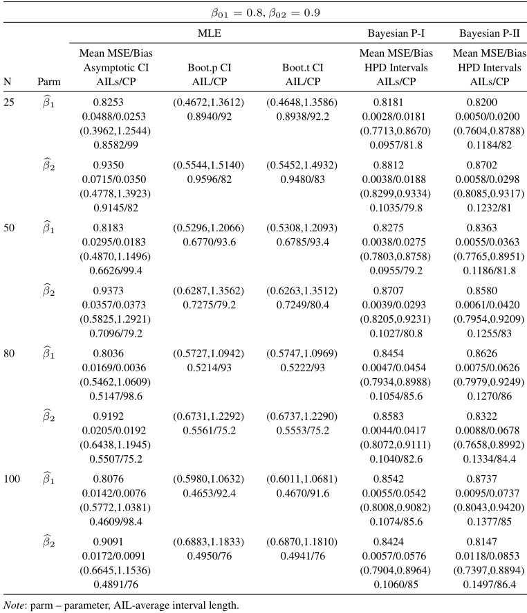
Table 10 Average estimated values, MSEs, bias, asymptotic and bootstrap (t-p) CI intervals of MLEs and BEs of IVT distribution parameters under random censoring data

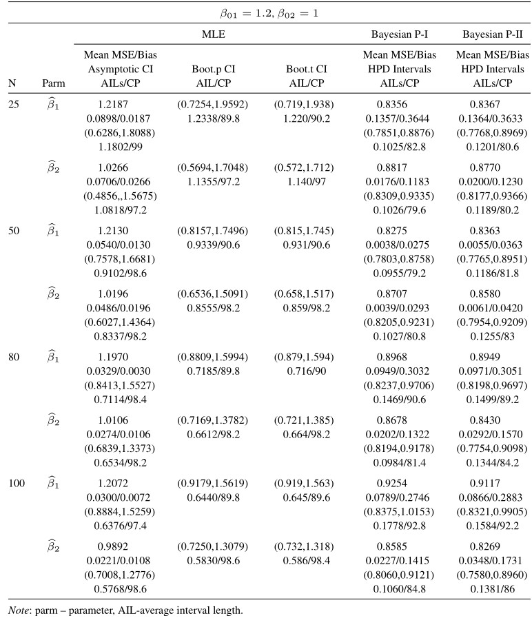
Table 11 Average estimated values, MSEs, bias, asymptotic and bootstrap (t-p) CI intervals of MLEs and BEs of IVT distribution parameters under random censoring data

From the results in Tables 8–11 the following conclusion can be made:

i. Similar to the complete case based on MSEs, higher values of $n$ lead to better estimates.

ii. The CPs of the MLEs are better than those of the CPs of Bayes estimates obtained under informative prior and the non-informative Bayes estimates, respectively.

iii. The MSEs of the MLEs are less than the BEs under the SEL function.

iv. It can be noticed that under informative prior the AILs and of HPD intervals are better than those of non-informative priors, Bootstrap (t – p), and MLEs.

v. Estimates obtained by the MLEs and BEs are almost unbiased.

4.6 Application to Real Data

In this section, the IVT distribution will be fitted to a real data set, to show how the IVT distribution can be applied in practice. These data are taken from a lung cancer study described by [12]. These data show remission times (in days) of a group of 15 patients. The data set is given as: (8, 10, 11, 25*, 42, 72, 82, 100*, 110, 118, 126, 144, 228, 314, 411). The observations with (*) sign the censored times. For this data set, the unknown parameter ($\beta$) of the IVT distribution will be estimated by the maximum-likelihood method, and with this, the estimate (MLE), the values of the Kolmogorov-Smirnov (KS) statistic (the distance between the empirical CDFs and the fitted CDFs), Akaike information criterion (AIC ), Bayesian information criterion (BIC) and Hannan-Quinn information criterion (HQIC) are calculated. These results are summarized in Table 12:

Table 12 The Values of Goodness of Fit Test for Lung Cancer Data Set to the IVT distribution

						k-s
Distribution	$\mathrm{B}$	$-$2log L	AIC	BIC	HQIC	D-statistics	p-value
IVT	0.277	299.65	301.7	302.2	301.5	0.3408	0.0751
IVT*	0.309	42.71	44.71	43.4	41.98	0.5452	0.4137
Note: (*) indicates the censoring times’ distribution.

From Table 12, the null hypothesis is not rejected, these lung cancer data may be modeled by the IVT distribution.

Moreover, MLE and Bayesian estimation methods are applied for estimating the model unknown parameter. For calculation of BEs, the hyper-parameters${\mathrm{a}}_1,{\mathrm{b}}_1,{\mathrm{a}}_2$ and ${\mathrm{b}}_2$ are chosen such that the expected value ${\mathrm{M}}_{{\beta }_1}$ of ${\beta }_1$ is 0.2437 with a variance ${\mathrm{V}}_{{\beta }_1}=0.0046$ giving ${\mathrm{a}}_1=13$ and ${\mathrm{b}}_1=53.34$, the expected value ${\mathrm{M}}_{{\beta }_2}$ of ${\beta }_2$ is 0.0375 with a variance ${\mathrm{V}}_{{\beta }_2}=0.0007$ giving ${\mathrm{a}}_2=2$ and ${\mathrm{b}}_2=53.33$. these results are listed in Table 13.

The empirical distribution for lifetimes and for censoring times for the lung cancer data are represented in Figures 7 and 8 respectively.

Table 13 The MLEs and BEs of the parameters from lung cancer data set

		BEs Under SEL Function		Confidence Intervals
					AILs (HPD Interval)
Parameter	MLEs	P-I	P-II	AILs (Asy CI)	P-I	P-II
${\widehat{\beta }}_1$	0.2437	0.2355	0.1761	0.2672 (0.1341,0.4012)	0.1284 (0.881,0.3165)	0.0533 (0.1494,0.2027)
${\widehat{\beta }}_2$	0.0375	0.0344	0.0321	0.1083 (0.0074,0.1158)	0.1083 (0.0232,0.0476)	0.0108 (0.027,0.0378)
Note: AILs- Average interval lengths.

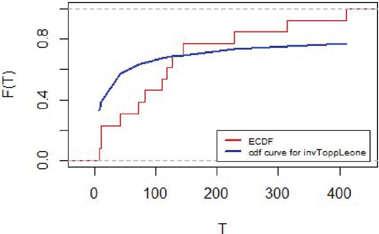
Figure 7 Empirical distribution for lifetimes for lung cancer data.

Furthermore, the inverted distributions defined in Section 3.5 can be used to fit this data also with numerical results listed in Table 14 and Figure 9.

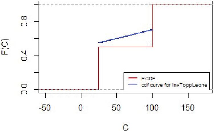
Figure 8 Empirical distribution for censoring times for lung cancer data.

Table 14 MLEs, AIC, BIC AICC and HQIC values, and Kolmogorov- Smirnov statistics for Lung Cancer Data lifetimes

		Measures
Model	MLE	p-value	K-S	$-$2log L	AIC	BIC	AICc	HQIC
IL	32.725	0.1052	0.3013	$-$195.5445	181.3550	182.0630	179.6216	181.3474
IE	36.90926	0.1051	0.3014	$-$179.3469	181.3469	182.0550	179.6136	181.3394
IR	0.824718	0.0000	0.5911	$-$179.3550	211.8932	212.6012	210.1599	211.8857

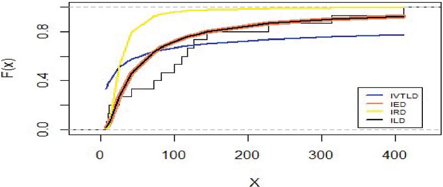
Figure 9 Empirical distribution for different lifetimes for lung cancer data.

5 Conclusion

In this paper, we have obtained the maximum likelihood estimates and Bayes estimates for the unknown parameter of the IVT distribution based on complete and random censoring data, the confidence intervals, HPD intervals, and bootstrap (p-t) intervals are also obtained. We perform some simulations to see the performances of the MLEs and BEs incomplete and random censoring data. One real data set has been re-analyzed based on random censoring data.

References

[1] Topp, C.W. and Leone, F.C. (1955). A family of J-shaped frequency functions, Journal of the American Statistical Association, 50, 209–219.

[2] Nadarajah, S. and Kotz, S. (2003). Moments of some J-shaped distributions, Journal of Applied Statistics, 30, 311–317.

[3] Ghitany, M.E., Kotz, S. and Xie, M. (2005). On some reliability measures and their stochastic ordering for the Topp–Leone distribution, Journal of Applied Statistics, 32, 715–722.

[4] Bayoud, H. (2016). Admissible minimax estimators for the shape parameter of Topp–Leone distribution, Communications in Statistics-Theory and Methods, doi: 10.1080/03610926.2013.818700.

[5] Muhammed, H.Z. (2019). On The Inverted Topp-Leone Distribution, international journal of reliability and applications, 20, 17–28.

[6] Dey, S., Singh, S., Tripathi, Y.M. and Asgharzadeh, A. (2016). Estimation and prediction for a progressively censored generalized inverted exponential distribution. Statistical Methodology, 132, 185–202.

[7] Ravenzwaaij, D.V., Cassey, P. and Brown, S.D. (2018). A simple introduction to Markov Chain Monte-Carlo sampling. Psychonomic Bulletin Review, 25, 143–154.

[8] Dey, S. and Pradhan, B. (2014). Generalized inverted exponential distribution under hybrid censoring. Statistical Methodology, 18, 101–114.

[9] Efron, B., and Tibshirani, R. J. (1993). An Introduction to the Bootstrap. New York: Chapman and Hall.

[10] Hall, P. (1988). Theoretical comparison of bootstrap confidence intervals. The Annals of Statistics, 927–953.

[11] Lawless, J. F. (2011). Statistical Models And Methods for Lifetime Data, Second edition. John Wiley & Sons, Inc, Canada.

[12] Kalbfleisch, J. D. and Prentice, R. L. (1980). The Statistical Analysis of Failure Time Data. New York: Wiley.

Biographies

Hiba Zeyada Muhammed received a bachelor’s degree in Statistics from the Faculty of Science at Cairo University in 2006, a master’s degree in Statistics from Cairo University in 2009, and philosophy of doctorate in statistics from Cairo University in 2013, respectively. She is currently working as an Associative Professor at the Department of Mathematical Statistics, Faculty of Graduate Studies for Statistical Research, Cairo University. Her research areas include Reliability, life testing, bivariate and multivariate analysis, copula modeling and ranked set sampling. She has been serving as a reviewer for many highly-respected journals.

Essam Abd Elsalam Muhammed received a bachelor’s degree in applied Statistics from the Faculty of Commerce at kafr El-sheikh University in 2015, a master’s degree in Statistics from Cairo University in 2020, and in the preparatory year of the doctorate in statistics at Cairo University, respectively. He is currently working as a teaching assistant at High Institute of Computer and Information Technology, Elshorouk Academy. his research areas include Reliability and life testing.

Journal of Reliability and Statistical Studies, Vol. 14, Issue 2 (2021), 615–650.
doi: 10.13052/jrss0974-8024.14212
© 2021 River Publishers