An Inferential Aptness of a Weibull Generated Distribution and Application

Brijesh P. Singh and Utpal Dhar Das^*

Department of Statistics, Institute of Science, Banaras Hindu University, Varanasi-221005, India

E-mail: utpal.statmath@gmail.com

*Corresponding Author

Received 31 July 2021; Accepted 11 November 2021; Publication 06 December 2021

Abstract

In this article an attempt has been made to develop a flexible single parameter continuous distribution using Weibull distribution. The Weibull distribution is most widely used lifetime distributions in both medical and engineering sectors. The exponential and Rayleigh distribution is particular case of Weibull distribution. Here in this study we use these two distributions for developing a new distribution. Important statistical properties of the proposed distribution is discussed such as moments, moment generating and characteristic function. Various entropy measures like Rényi, Shannon and cumulative entropy are also derived. The $k^{th}$ order statistics of pdf and cdf also obtained. The properties of hazard function and their limiting behavior is discussed. The maximum likelihood estimate of the parameter is obtained that is not in closed form, thus iteration procedure is used to obtain the estimate. Simulation study has been done for different sample size and MLE, MSE, Bias for the parameter $\lambda$ has been observed. Some real data sets are used to check the suitability of model over some other competent distributions for some data sets from medical and engineering science. In the tail area, the proposed model works better. Various model selection criterion such as -2LL, AIC, AICc, BIC, K-S and A-D test suggests that the proposed distribution perform better than other competent distributions and thus considered this as an alternative distribution. The proposed single parameter distribution is found more flexible as compare to some other two parameter complicated distributions for the data sets considered in the present study.

Keywords: Bonferroni and Gini coefficient, K-S test, MLE, Moments, MRLF, Rényi and Shannon entropy.

1 Introduction

The exponentiated exponential, Weibull, Gamma, Lognormal distribution and their weighted version have an extensive usage in the fields of medical and engineering sciences. Some weighted distributions defined in the statistical literature, for example the weighted inverted exponential distribution [18], weighted Weibull distribution [19] and [25], weighted multivariate normal distribution [15], weighted inverse Weibull distribution [17], weighted three parameter Weibull distribution [2]. A two parameter weighted exponential distribution introduced [21] based on a modified weighted version of Azzalini’s approach [3]. A two parameter general class of distribution based on Lindley and a compounded exponential distribution with Lindley distribution for decreasing hazard has been discussed and apply to the real data sets [6] and [7].

The Rayleigh distribution is a particular form of two parameter Weibull distribution and widely used to model, events that occur in different fields of natural sciences. The generalized Rayleigh distribution is studied [14], [27] and [20]. Recently [16] observed that the two parameter generalized Rayleigh distribution that can be used quite effectively in modeling strength and life time data. Different methods to estimate the unknown parameters of the generalized Rayleigh and discussed several interesting properties [11]. The Weibull Rayleigh distribution developed [12] and derived its statistical properties. Exponentiated inverse Rayleigh distribution (EIRD) was introduced [13] and discussed its various statistical properties and it is a generalized form of inverse Rayleigh distribution [24]. A two parameter model introduced [1] as a competitive extension for Rayleigh distribution using the TIHL-G distributions and defined it as type 1 half-logistic Rayleigh distribution (TIHLR) and discussed its statistical properties and simulation studies.

A random variable $X$ is said to have a mixture of two distributions ${\varphi }_1(x)$ and ${\varphi }_2(x)$ if its probability distribution is given by

$f(x)={\eta }_1{\varphi }_1(x)+{\eta }_2{\varphi }_2(x)$

where ${\eta }_1$ and ${\eta }_2$ are two positive number such that ${\eta }_1+{\eta }_2=1$.

In this paper an attempt has been made to develop a single parameter continuous distribution on the same logic what has been used in the process of development of Lindley distribution. Therefore in this study, exponential and Rayleigh distribution have been mixed with a suitable mixing parameter. Its first four moments, mean residual life function hazard function and various entropy has been discussed. Estimation of the parameter has been discussed and the suitability of distribution is tested on some real data set.

2 Proposed Continuous Distribution

The probability density function (pdf) of Weibull distribution is given by

$$f_w(x;k,\lambda )=\lambda k{x}^{k-1}{e}^{-\lambda x^k}$$

(1)

In the above equation, if we put $k=1$, the distribution become exponential distribution and for $k=2$, the distribution become Rayleigh distribution.

Now we consider mixing parameter as $p=\frac{\lambda }{\lambda +\alpha }$, we have

$f(x)$	$=pf(x;1,\lambda )+(1-p)f(x;2,\lambda )$
	$={\displaystyle \frac{\lambda }{\lambda +\alpha }}\lambda e^{-\lambda x}+{\displaystyle \frac{\alpha }{\lambda +\alpha }}2\lambda x{e}^{-\lambda x^2}$
	$={\displaystyle \frac{\lambda }{\lambda +\alpha }}{e}^{-\lambda x}\left(\lambda +2\alpha x{e}^{-\lambda x(x-1)}\right);\alpha >0,\lambda >0$	(2)

If $\alpha =0$ in the Equation (2), we have an exponential distribution and if $\alpha =1$ in the Equation (2), we have a mixture of exponential and Rayleigh distribution with mixing proportion $\frac{\lambda }{\lambda +1}$. This distribution is named as Rayleigh-exponential distribution (RED) and the pdf is given as

$f(x)={\displaystyle \frac{\lambda }{\lambda +1}}{e}^{-\lambda x}\left(\lambda +2x{e}^{-\lambda x(x-1)}\right);\lambda >0$

(3)

The plot of pdf of RED is given as

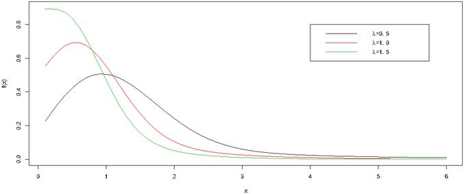
Figure 1 Probability density function of RED.

The cdf of RED is given by

$F(x;\lambda )={\displaystyle {\int }_0^x}f(t)\mathit{d}t=1-{\displaystyle \frac{\lambda e^{-\lambda x}+e^{-\lambda x^2}}{\lambda +1}}$

(4)

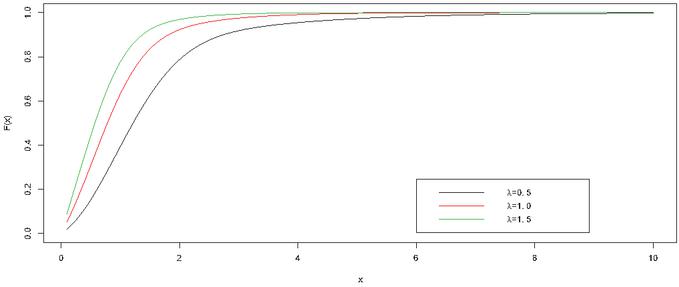
Figure 2 Cumulative distribution function of RED.

The survival function $S(t)$, which is a probability that a patient or item will survive beyond any specified time $t$.

$S(t)=1-F(t)={\displaystyle \frac{\lambda e^{-\lambda t}+e^{-\lambda t^2}}{\lambda +1}}$

(5)

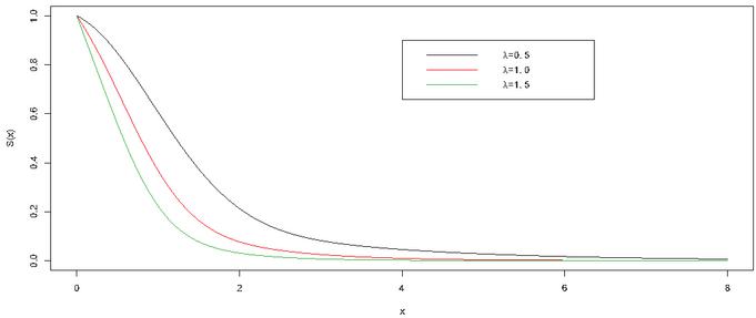
Figure 3 Survival function of RED.

and the corresponding hazard function of RED distribution is given by

$h(x)={\displaystyle \frac{f(x)}{1-F(x)}}={\displaystyle \frac{\lambda \left(\lambda +2x{e}^{-\lambda x(x-1)}\right)}{\left(\lambda +e^{-\lambda x(x-1)}\right)}}$

(6)

Now from Equation (6)

$\underset{x\to 0}{lim}h(x)$	$={\displaystyle \frac{{\lambda }^2}{\lambda +1}}$	(7)
$\underset{x\to \frac{1}{\lambda }}{lim}h(x)$	$={\displaystyle \frac{\left({\lambda }^2+2e^{-(\frac{1}{\lambda }-1)}\right)}{\left(\lambda +e^{-(\frac{1}{\lambda }-1)}\right)}}$	(8)
$\underset{x\to \mathrm{\infty }}{lim}h(x)$	$=\lambda$	(9)

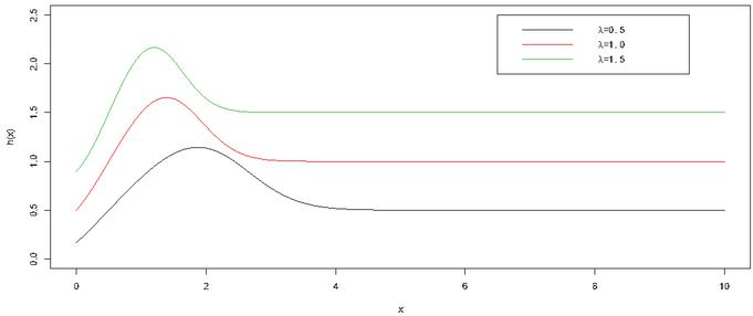
Figure 4 Hazard function of RED.

From Equations (7), (8), (9) and Figure 4, we can say that the hazard of RED is first increasing then decreasing and finally it become constant.

3 Moments

The $r^{th}$ order moments is given by

$E(X^r)$	$={\displaystyle {\int }_0^{\mathrm{\infty }}}{x}^{r}f(x)\mathit{d}x={\displaystyle {\int }_0^{\mathrm{\infty }}}{x}^r{\displaystyle \frac{\lambda }{\lambda +1}}{e}^{-\lambda x}\left(\lambda +2x{e}^{-\lambda x(x-1)}\right)\mathit{d}x$
	$={\displaystyle \frac{{\lambda }^2}{\lambda +1}}{\displaystyle {\int }_0^{\mathrm{\infty }}}{x}^r{e}^{-\lambda x}\mathit{d}x+{\displaystyle \frac{1}{(\lambda +1){\lambda }^{\frac{r}{2}}}}{\displaystyle {\int }_0^{\mathrm{\infty }}}{(\lambda x^2)}^{\frac{r}{2}}{e}^{-\lambda x^2}d(\lambda x^2)$
	$={\displaystyle \frac{{\lambda }^2}{\lambda +1}}{\displaystyle \frac{\mathrm{\Gamma }(r+1)}{{\lambda }^{r+1}}}+{\displaystyle \frac{\mathrm{\Gamma }\left(\frac{r}{2}+1\right)}{(\lambda +1){\lambda }^{\frac{r}{2}}}}={\displaystyle \frac{\lambda }{\lambda +1}}\left({\displaystyle \frac{r!}{{\lambda }^r}}\right)+{\displaystyle \frac{\left(\frac{r}{2}\right)!}{(\lambda +1){\lambda }^{\frac{r}{2}}}}$	(10)

Now the moments of the distribution is obtained as

$E(X)=$	${\displaystyle \frac{1}{\lambda +1}}\left(1+{\displaystyle \frac{1}{2}}\sqrt{{\displaystyle \frac{\pi }{\lambda }}}\right)$	(11)
$E(X^2)=$	${\displaystyle \frac{3}{\lambda (\lambda +1)}}$	(12)
$E(X^3)=$	${\displaystyle \frac{3}{\lambda (\lambda +1)}}\left({\displaystyle \frac{2}{\lambda }}+{\displaystyle \frac{1}{4}}\sqrt{{\displaystyle \frac{\pi }{\lambda }}}\right)$	(13)
$E(X^4)=$	${\displaystyle \frac{2}{{\lambda }^2(\lambda +1)}}\left(1+{\displaystyle \frac{12}{\lambda }}\right)$	(14)
$V(X)=E(X^2)-{\left(E(X)\right)}^2=$	${\displaystyle \frac{1}{\lambda +1}}\left[{\displaystyle \frac{3}{\lambda }}-{\displaystyle \frac{1}{\lambda +1}}{\left(1+{\displaystyle \frac{1}{2}}\sqrt{{\displaystyle \frac{\pi }{\lambda }}}\right)}^2\right]$	(15)

Median of the distribution is given by the equation

${\displaystyle {\int }_0^M}{\displaystyle \frac{\lambda }{\lambda +1}}{e}^{-\lambda x}\left(\lambda +2x{e}^{-\lambda x(x-1)}\right)={\displaystyle \frac{1}{2}}$	(16)
$\text{i.e}\mathit{\hspace{1em}}{\displaystyle \frac{e^{-\lambda M}}{\lambda +1}}\left(\lambda +e^{-\lambda M(M-1)}\right)={\displaystyle \frac{1}{2}}$	(17)

This is a non linear equation we can solve it by numerically.

4 Quantile Function

The quantile function $x_q$ of RED is the real solution of the equation given below

$F(x_q)$	$=p$
$(\lambda +1)(1-p)e^{\lambda x_q}$	$=\lambda +e^{-\lambda \left[{(x_q-\frac{1}{2})}^2-\frac{1}{4}\right]}$	(18)

The equation is not in closed form thus the solution of $x_q$ may obtain iteratively. If $q=0.5$ in the above equation, we can get median of the distribution.

5 Generating Function

Theorem 1 Moment generating function of RED is given by

${\displaystyle \frac{{\lambda }^2}{(\lambda +1)(\lambda -t)}}+{\displaystyle \frac{1}{\lambda +1}}+{\displaystyle \frac{t{e}^{\frac{t^2}{4\lambda }}}{2\sqrt{\lambda }(\lambda +1)}}\mathrm{\Gamma }({\displaystyle \frac{1}{2}},{\displaystyle \frac{t^2}{4\lambda }})$

Proof:  

$M_x(t)={\displaystyle {\int }_0^{\mathrm{\infty }}}{e}^{tx}f(x)\mathit{d}x={\displaystyle \frac{\lambda }{\lambda +1}}{\displaystyle {\int }_0^{\mathrm{\infty }}}{e}^{-(\lambda -t)x}\left(\lambda +2x{e}^{-\lambda x(x-1)}\right)\mathit{d}x$

Now

	${\displaystyle \frac{{\lambda }^2}{(\lambda +1)(\lambda -t)}}{\displaystyle {\int }_0^{\mathrm{\infty }}}{e}^{-(\lambda -t)x}d\left((\lambda -t)x\right)$
	$\mathrm{\hspace{1em}\hspace{1em}}+{\displaystyle \frac{\lambda }{\lambda +1}}{\displaystyle {\int }_0^{\mathrm{\infty }}}2x{e}^{-x(\lambda x-t)}\mathit{d}x$
$=$	${\displaystyle \frac{{\lambda }^2}{(\lambda +1)(\lambda -t)}}+{\displaystyle \frac{1}{\lambda +1}}{\displaystyle {\int }_0^{\mathrm{\infty }}}{e}^{-x(\lambda x-t)}d(x(\lambda x-t))$
	$\mathrm{\hspace{1em}\hspace{1em}}+{\displaystyle \frac{t}{\lambda +1}}{\displaystyle {\int }_0^{\mathrm{\infty }}}{e}^{-x(\lambda x-t)}\mathit{d}x$

After simplification on last integral we get,

${\displaystyle \frac{{\lambda }^2}{(\lambda +1)(\lambda -t)}}+{\displaystyle \frac{1}{\lambda +1}}$
$\mathrm{\hspace{1em}\hspace{1em}}+{\displaystyle \frac{t{e}^{\frac{t^2}{4\lambda }}}{\sqrt{\lambda }(\lambda +1)}}{\displaystyle {\int }_0^{\mathrm{\infty }}}{e}^{-{\left(x\sqrt{\lambda }-\frac{t}{2\sqrt{\lambda }}\right)}^2}d\left[\left(x\sqrt{\lambda }-{\displaystyle \frac{t}{2\sqrt{\lambda }}}\right)\right]$	(19)

Now let ${(x\sqrt{\lambda }-\frac{t}{2\sqrt{\lambda }})}^2=z,\text{we have}\mathrm{\hspace{0.25em}2}(x\sqrt{\lambda }-\frac{t}{2\sqrt{\lambda }})d(x\sqrt{\lambda }-\frac{t}{2\sqrt{\lambda }})=dz$, also $x\to 0,z\to \frac{t^2}{4\lambda }$ and $x\to \mathrm{\infty },z\to \mathrm{\infty }$.

${\displaystyle \frac{{\lambda }^2}{(\lambda +1)(\lambda -t)}}+{\displaystyle \frac{1}{\lambda +1}}+{\displaystyle \frac{t{e}^{\frac{t^2}{4\lambda }}}{2\sqrt{\lambda }(\lambda +1)}}{\displaystyle {\int }_{\frac{t^2}{4\lambda }}^{\mathrm{\infty }}}{z}^{\frac{1}{2}-1}{e}^{-z}\mathit{d}z$

(20)

Where $\mathrm{\Gamma }(s,x)={\int }_x^{\mathrm{\infty }}{t}^{s-1}{e}^{-t}\mathit{d}t$ is upper incomplete gamma function. Finally from (20) we get our required results as

${\displaystyle \frac{{\lambda }^2}{(\lambda +1)(\lambda -t)}}+{\displaystyle \frac{1}{\lambda +1}}+{\displaystyle \frac{t{e}^{\frac{t^2}{4\lambda }}}{2\sqrt{\lambda }(\lambda +1)}}\mathrm{\Gamma }({\displaystyle \frac{1}{2}},{\displaystyle \frac{t^2}{4\lambda }})$

(21)

Corollary 1 If we replace $i\mathit{}t$ for $t$ in equation number (21) we get the characteristic function as

${\mathrm{\Phi }}_x(t)$	$={\displaystyle {\int }_0^{\mathrm{\infty }}}{e}^{itx}f(x)\mathit{d}x$
	$={\displaystyle \frac{{\lambda }^2}{(\lambda +1)(\lambda -it)}}+{\displaystyle \frac{1}{\lambda +1}}+{\displaystyle \frac{it{e}^{\frac{-t^2}{4\lambda }}}{2\sqrt{\lambda }(\lambda +1)}}\mathrm{\Gamma }({\displaystyle \frac{1}{2}},{\displaystyle \frac{-t^2}{4\lambda }})$	(22)

6 Bonferroni and Lorenz Curves

The Bonferroni, Lorenz curves and Bonferroni, Gini indices have applications not only in economics to study the income and poverty, but also in other fields like reliability, insurance, medical and demography. The Bonferroni [8] and Lorenz curves are defined by

$B(p)={\displaystyle \frac{1}{p\mu }}{\displaystyle {\int }_0^q}xf(x)\mathit{d}x\mathit{\hspace{1em}}\text{and}\mathit{\hspace{1em}}L(p)={\displaystyle \frac{1}{\mu }}{\displaystyle {\int }_0^q}xf(x)\mathit{d}x$

(23)

Respectively where, $\mu =E(x)$ and $q=F^{-1}(p)$. The Bonferroni and Gini indices are defined by

$B=1-{\displaystyle {\int }_0^1}B(p)\mathit{d}p\mathit{\hspace{1em}}\text{and}\mathit{\hspace{1em}}G=1-2{\displaystyle {\int }_0^1}L(p)\mathit{d}p$

(24)

Here

$B(p)$	$={\displaystyle \frac{1}{p\mu }}{\displaystyle \frac{\lambda }{\lambda +1}}{\displaystyle {\int }_0^q}x{e}^{-\lambda x}\left(\lambda +2x{e}^{-\lambda x(x-1)}\right)\mathit{d}x$
	$={\displaystyle \frac{1}{p\mu }}{\displaystyle \frac{1}{\lambda +1}}{\displaystyle {\int }_0^q}(\lambda x)e^{-(\lambda x)}d(\lambda x)+{\displaystyle \frac{1}{p\mu }}{\displaystyle \frac{1}{\lambda +1}}{\displaystyle {\int }_0^q}2\lambda x^2{e}^{-\lambda x^2}\mathit{d}x$
	$={\displaystyle \frac{1}{p\mu }}{\displaystyle \frac{1}{\lambda +1}}\left[1-(1+\lambda q)e^{-(\lambda q)}\right]+{\displaystyle \frac{1}{p\mu }}{\displaystyle \frac{1}{\lambda +1}}{I}_1$	(25)

Now let $\lambda x^2=z$; $2\lambda xdx=dz⟹2dx=\frac{dz}{\sqrt{\lambda z}}$ and $x\to 0,z\to 0$; $x\to q,z\to \lambda q^2$

$I_1={\displaystyle \frac{1}{\sqrt{\lambda }}}{\displaystyle {\int }_0^{\lambda q^2}}\sqrt{z}{e}^{-z}\mathit{d}z⟹I_1=-q{e}^{-\lambda q^2}+{\displaystyle \frac{1}{\sqrt{\lambda }}}{\displaystyle {\int }_0^{\lambda q^2}}{\displaystyle \frac{e^{-z}}{2\sqrt{z}}}\mathit{d}z$

(26)

Let $\sqrt{z}=u;\frac{dz}{2\sqrt{z}}=du;z\to 0,u\to 0;z\to \lambda q^2,u\to q\sqrt{\lambda }$, then

$I_1=-q{e}^{-\lambda q^2}+{\displaystyle \frac{1}{\sqrt{\lambda }}}{\displaystyle {\int }_0^{q\sqrt{\lambda }}}{e}^{-u^2}\mathit{d}u=-q{e}^{-\lambda q^2}+{\displaystyle \frac{1}{\sqrt{\lambda }}}{\displaystyle \frac{\sqrt{\pi }}{2}}\mathbf{\text{erf}}(q\sqrt{\lambda })$

(27)

Since,

$\mathbf{\text{erf}}(x)={\displaystyle \frac{2}{\sqrt{\pi }}}{\displaystyle {\int }_0^x}{e}^{-t^2}\mathit{d}t$

Now from (6) and (27) we get the expression of Bonferroni curve

$B(p)$	$={\displaystyle \frac{1}{p\mu }}{\displaystyle \frac{1}{\lambda +1}}\left[\left[1-(1+\lambda q)e^{-(\lambda q)}\right]+\left({\displaystyle \frac{1}{2}}\sqrt{{\displaystyle \frac{\pi }{\lambda }}}\mathbf{\text{erf}}(q\sqrt{\lambda })-q{e}^{-(\lambda q^2)}\right)\right]$
	$={\displaystyle \frac{\left[\left[1-(1+\lambda q)e^{-(\lambda q)}\right]+\left(\frac{1}{2}\sqrt{\frac{\pi }{\lambda }}\mathbf{\text{erf}}(q\sqrt{\lambda })-q{e}^{-(\lambda q^2)}\right)\right]}{p\left(1+\frac{1}{2}\sqrt{\frac{\pi }{\lambda }}\right)}}$	(28)

where $\mu =\frac{1}{\lambda +1}(1+\frac{1}{2}\sqrt{\frac{\pi }{\lambda }})$, mean of the distribution and the Lorenz curve is obtained as

$L(p)={\displaystyle \frac{\left[\left[1-(1+\lambda q)e^{-(\lambda q)}\right]+\left(\frac{1}{2}\sqrt{\frac{\pi }{\lambda }}\mathbf{\text{erf}}(q\sqrt{\lambda })-q{e}^{-(\lambda q^2)}\right)\right]}{\left(1+\frac{1}{2}\sqrt{\frac{\pi }{\lambda }}\right)}}$

(29)

7 Mean Residual Life Function

The mean residual life function is defined by

$m(x)$	$=E[X-x|X>x]={\displaystyle \frac{1}{1-F(x)}}{\displaystyle {\int }_x^{\mathrm{\infty }}}[1-F(t)]\mathit{d}t$
	$={\displaystyle {\int }_x^{\mathrm{\infty }}}{\displaystyle \frac{\lambda e^{-\lambda t}+e^{-\lambda t^2}}{\lambda +1}}\mathit{d}t$
	$={\displaystyle \frac{1}{\lambda +1}}{\displaystyle {\int }_x^{\mathrm{\infty }}}{e}^{-\lambda t}d(\lambda t)+{\displaystyle \frac{1}{\lambda +1}}{\displaystyle {\int }_x^{\mathrm{\infty }}}{e}^{-\lambda t^2}\mathit{d}t$

Now let $\lambda t^2=z$; $2\lambda tdt=dz⟹2dt=\frac{dz}{\sqrt{\lambda z}}$ and $t\to x,z\to \lambda x^2$; $t\to \mathrm{\infty },z\to \mathrm{\infty }$

${\displaystyle \frac{e^{-\lambda x}}{\lambda +1}}+{\displaystyle \frac{1}{\lambda +1}}{\displaystyle {\int }_{\lambda x^2}^{\mathrm{\infty }}}{\displaystyle \frac{e^{-z}}{2\sqrt{\lambda z}}}\mathit{d}z\mathit{\hspace{1em}}\text{i.e}$
${\displaystyle \frac{e^{-\lambda x}}{\lambda +1}}+{\displaystyle \frac{1}{2\sqrt{\lambda }(\lambda +1)}}{\displaystyle {\int }_{\lambda x^2}^{\mathrm{\infty }}}{z}^{-\frac{1}{2}}{e}^{-z}\mathit{d}z$	(30)

Now from (7) the MRLF obtained as

$m(x)={\displaystyle \frac{e^{-\lambda x}}{\lambda +1}}+{\displaystyle \frac{\mathrm{\Gamma }(\lambda x^2,\frac{1}{2})}{2\sqrt{\lambda }(\lambda +1)}}$

(31)

Now if we put $x=0$ in equation number (31) then we get $m(0)=\frac{1}{\lambda +1}\left(1+\frac{1}{2}\sqrt{\frac{\pi }{\lambda }}\right)$, which is mean of the distribution and $\mathrm{\Gamma }(*,*)$ is the upper incomplete gamma function.

8 Rényi Entropy

We know that the entropy is a measure of uncertainty. In 1960, Rényi [5] defined a generalization of Shannon entropy which depends on a parameter and it is defined by,

$e(\eta )$	$={\displaystyle \frac{1}{1-\eta }}\log \left[{\displaystyle {\int }_0^{\mathrm{\infty }}}{f}^{\eta }(x)\mathit{d}x\right]$
	$={\displaystyle \frac{1}{1-\eta }}\log \left[{\displaystyle {\int }_0^{\mathrm{\infty }}}{\left({\displaystyle \frac{\lambda }{\lambda +1}}\right)}^{\eta }{e}^{-\eta \lambda x}{\left[\lambda +2x{e}^{-\lambda x(x-1)}\right]}^{\eta }\mathit{d}x\right]$
	$={\displaystyle \frac{1}{1-\eta }}\log {\displaystyle \frac{{\lambda }^{2\eta }}{{(\lambda +1)}^{\eta }}}\left[{\displaystyle {\int }_0^{\mathrm{\infty }}}{e}^{-\eta \lambda x}{\left[1+{\displaystyle \frac{2x{e}^{-\lambda x(x-1)}}{\lambda }}\right]}^{\eta }\mathit{d}x\right]$(32)

Now applying binomial expansion ${(1+x)}^n={\sum }_{k=0}^n\left(\genfrac{}{}{0pt}{}{n}{k}\right)x^k$ from above equation we get

$={\displaystyle \frac{1}{1-\eta }}\log {\displaystyle \frac{{\lambda }^{2\eta }}{{(\lambda +1)}^{\eta }}}{\displaystyle {\int }_0^{\mathrm{\infty }}}{e}^{-\eta \lambda x}{\displaystyle \sum _{k=0}^{\eta }}\left({\displaystyle \genfrac{}{}{0pt}{}{\eta }{k}}\right){\left({\displaystyle \frac{2x{e}^{-\lambda x(x-1)}}{\lambda }}\right)}^{k}dx$

$={\displaystyle \frac{1}{1-\eta }}\log {\displaystyle \frac{{\lambda }^{2\eta }}{{(\lambda +1)}^{\eta }}}{\displaystyle \sum _{k=0}^{\eta }}\left({\displaystyle \genfrac{}{}{0pt}{}{\eta }{k}}\right){\left({\displaystyle \frac{2}{\lambda }}\right)}^k\left[{\displaystyle {\int }_0^{\mathrm{\infty }}}{x}^k{e}^{-(\eta -k)\lambda x}{e}^{-k\lambda x^2}\mathit{d}x\right]$

Using $e^{-x}={\sum }_{k=0}^{\mathrm{\infty }}\frac{{(-x)}^k}{k!}$, we get

$={\displaystyle \frac{1}{1-\eta }}\log {\displaystyle \frac{{\lambda }^{2\eta }}{{(\lambda +1)}^{\eta }}}{\displaystyle \sum _{k=0}^{\eta }}\left({\displaystyle \genfrac{}{}{0pt}{}{\eta }{k}}\right){\left({\displaystyle \frac{2}{\lambda }}\right)}^k$

$\mathrm{\hspace{1em}}\times \left[{\displaystyle {\int }_0^{\mathrm{\infty }}}{x}^k{e}^{-(\eta -k)\lambda x}{\displaystyle \sum _{l=0}^{\mathrm{\infty }}}{(-1)}^l{\displaystyle \frac{{(k\lambda x^2)}^l}{l!}}dx\right]$

$={\displaystyle \frac{1}{1-\eta }}\log {\displaystyle \frac{{\lambda }^{2\eta }}{{(\lambda +1)}^{\eta }}}{\displaystyle \sum _{k=0}^{\eta }}\left({\displaystyle \genfrac{}{}{0pt}{}{\eta }{k}}\right){\left({\displaystyle \frac{2}{\lambda }}\right)}^k{\displaystyle \sum _{l=0}^{\mathrm{\infty }}}{(-1)}^l{\displaystyle \frac{{(k\lambda )}^l}{l!}}$

$\mathrm{\hspace{1em}}\times \left[{\displaystyle {\int }_0^{\mathrm{\infty }}}{x}^{k+2l}{e}^{-(\eta -k)\lambda x}\mathit{d}x\right]$

After simplification we get our required expression.

$e(\eta )$	$={\displaystyle \frac{1}{1-\eta }}\log [{\displaystyle \frac{{\lambda }^{2\eta }}{{(\lambda +1)}^{\eta }}}{\displaystyle \sum _{k=0}^{\eta }}{\displaystyle \sum _{l=0}^{\mathrm{\infty }}}{(-1)}^l\left({\displaystyle \genfrac{}{}{0pt}{}{\eta }{k}}\right){\left({\displaystyle \frac{2}{\lambda }}\right)}^k$
	$\mathrm{\hspace{1em}}{\displaystyle \frac{{(k\lambda )}^l}{l!}}{\displaystyle \frac{\mathrm{\Gamma }(k+2l+1)}{{\left\{(\eta -k)\lambda \right\}}^{k+2l+1}}}]$

8.1 Cumulative Residual Entropy

Cumulative residual entropy is defined as

${\mathrm{{\rm Y}}}_{CR}$	$=-{\displaystyle {\int }_0^{\mathrm{\infty }}}Pr(X>x)\log Pr(X>x)dx$
	$=-{\displaystyle {\int }_0^{\mathrm{\infty }}}\left({\displaystyle \frac{\lambda e^{-\lambda x}+e^{-\lambda x^2}}{\lambda +1}}\right)\log \left({\displaystyle \frac{\lambda e^{-\lambda x}+e^{-\lambda x^2}}{\lambda +1}}\right)\mathit{d}x$
	$=-{\displaystyle {\int }_0^{\mathrm{\infty }}}\left({\displaystyle \frac{\lambda e^{-\lambda x}+e^{-\lambda x^2}}{\lambda +1}}\right)$
	$\mathrm{\hspace{1em}}\times \left[\log \left({\displaystyle \frac{\lambda }{\lambda +1}}\right)-\lambda x+\log \left(1+{\displaystyle \frac{e^{-\lambda x^2+\lambda x}}{\lambda }}\right)\right]dx$
	$={\displaystyle \frac{-1}{\lambda +1}}\log \left({\displaystyle \frac{\lambda }{\lambda +1}}\right){\displaystyle {\int }_0^{\mathrm{\infty }}}\left(\lambda e^{-\lambda x}+e^{-\lambda x^2}\right)\mathit{d}x$
	$\mathrm{\hspace{1em}}+{\displaystyle \frac{\lambda }{\lambda +1}}{\displaystyle {\int }_0^{\mathrm{\infty }}}x\left(\lambda e^{-\lambda x}+e^{-\lambda x^2}\right)\mathit{d}x$
	$\mathrm{\hspace{1em}}-{\displaystyle \frac{\lambda }{\lambda +1}}{\displaystyle {\int }_0^{\mathrm{\infty }}}\left(\lambda e^{-\lambda x}+e^{-\lambda x^2}\right)\log \left(1+{\displaystyle \frac{e^{-\lambda x^2+\lambda x}}{\lambda }}\right)\mathit{d}x$(33)

Applying logarithmic expansion $\log (1+x)={\sum }_{k=1}^{\mathrm{\infty }}{(-1)}^{k-1}\frac{x^k}{k}$ on last part of integrand of equation number (33), we get

$=-{\displaystyle \frac{1}{\lambda +1}}\log \left({\displaystyle \frac{\lambda }{\lambda +1}}\right)\left(1+{\displaystyle \frac{1}{2}}\sqrt{{\displaystyle \frac{\pi }{\lambda }}}\right)+{\displaystyle \frac{1}{\lambda +1}}{\displaystyle {\int }_0^{\mathrm{\infty }}}(\lambda x)e^{-(\lambda x)}d(\lambda x)$

$\mathrm{\hspace{1em}}+{\displaystyle \frac{1}{2(\lambda +1)}}{\displaystyle {\int }_0^{\mathrm{\infty }}}{e}^{-(\lambda x^2)}d(\lambda x^2)-{\displaystyle \frac{1}{\lambda +1}}{\displaystyle {\int }_0^{\mathrm{\infty }}}\left(\lambda e^{-\lambda x}+e^{-\lambda x^2}\right)$

$\mathrm{\hspace{1em}}{\displaystyle \sum _{k=1}^{\mathrm{\infty }}}{\displaystyle \frac{{(-1)}^{k-1}}{k{\lambda }^k}}{\displaystyle {\int }_0^{\mathrm{\infty }}}\left(\lambda e^{-\lambda x}+e^{-\lambda x^2}\right)e^{-k\left(\lambda e^{-\lambda x}+e^{-\lambda x^2}\right)}\mathit{d}x$

After simplification we obtained the cumulative residual entropy as

${\mathrm{{\rm Y}}}_{CR}$

$=-{\displaystyle \frac{1}{\lambda +1}}\log \left({\displaystyle \frac{\lambda }{\lambda +1}}\right)\left(1+{\displaystyle \frac{1}{2}}\sqrt{{\displaystyle \frac{\pi }{\lambda }}}\right)$

$\mathrm{\hspace{1em}}+{\displaystyle \frac{1}{3(\lambda +1)}}{\displaystyle \frac{1}{2}}\sqrt{{\displaystyle \frac{\pi }{\lambda }}}{\displaystyle \sum _{k=1}^{\mathrm{\infty }}}{\displaystyle \frac{{(-1)}^{k-1}}{k{\lambda }^k}}\left\{{\displaystyle \frac{\lambda e^{\lambda k{\left(\frac{k-1}{2k}\right)}^2}}{\sqrt{k}}}+{\displaystyle \frac{e^{\left(\frac{\lambda k^2}{4(k+1)}\right)}}{\sqrt{k+1}}}\right\}$

8.2 Shannon Entropy

Shannon entropy introduced by Shannon [9] is a limiting case of Rényi entropy it is widely used in Physics. The Rényi entropy tends to Shannon entropy as $\eta \to 0$.

$E(-\log f(x))=-{\displaystyle {\int }_0^{\mathrm{\infty }}}f(x)\log f(x)\mathit{d}x$

(34)

Now from (2) we get

${\displaystyle {\int }_0^{\mathrm{\infty }}}\left[\log \left({\displaystyle \frac{\lambda }{\lambda +1}}\right)-\lambda x+\log \left(\lambda +2x{e}^{-\lambda x(x-1)}\right)\right]f(x)\mathit{d}x$

$\mathrm{\hspace{1em}\hspace{1em}}=\log \left({\displaystyle \frac{\lambda }{\lambda +1}}\right){\displaystyle {\int }_0^{\mathrm{\infty }}}f(x)\mathit{d}x-\lambda E(x)$

$\mathrm{\hspace{1em}\hspace{1em}}\mathit{\hspace{1em}}+\log \lambda {\displaystyle {\int }_0^{\mathrm{\infty }}}f(x)\mathit{d}x+{\displaystyle {\int }_0^{\mathrm{\infty }}}\log \left[1+{\displaystyle \frac{2x{e}^{-\lambda x(x-1)}}{\lambda }}\right]f(x)\mathit{d}x$

Applying logarithmic expansion $\log (1+x)={\sum }_{k=1}^{\mathrm{\infty }}{(-1)}^{k-1}\frac{x^k}{k}$ we get

$\log \left({\displaystyle \frac{{\lambda }^2}{\lambda +1}}\right)-{\displaystyle \frac{\lambda }{\lambda +1}}\left(1+{\displaystyle \frac{1}{2}}\sqrt{{\displaystyle \frac{\pi }{\lambda }}}\right)$

$\mathrm{\hspace{1em}\hspace{1em}}+{\displaystyle \frac{\lambda }{\lambda +1}}{\displaystyle \sum _{k=0}^{\mathrm{\infty }}}{\displaystyle \frac{{(-1)}^{k-1}{2}^k}{k{\lambda }^k}}{\displaystyle {\int }_0^{\mathrm{\infty }}}{x}^k{e}^{-k\lambda x(x-1)}\left[\lambda e^{-\lambda x}+2x{e}^{-\lambda x^2}\right]\mathit{d}x$

Now applying $e^{-x}={\sum }_{m=0}^{\mathrm{\infty }}{(-1)}^m\frac{x^m}{m!}$, we get

$\log \left({\displaystyle \frac{{\lambda }^2}{\lambda +1}}\right)-{\displaystyle \frac{\lambda }{\lambda +1}}\left(1+{\displaystyle \frac{1}{2}}\sqrt{{\displaystyle \frac{\pi }{\lambda }}}\right)+{\displaystyle \frac{\lambda }{\lambda +1}}{\displaystyle \sum _{k=0}^{\mathrm{\infty }}}{\displaystyle \frac{{(-1)}^{k-1}{2}^k}{k{\lambda }^k}}$
$\mathrm{\hspace{1em}\hspace{1em}}{\displaystyle {\int }_0^{\mathrm{\infty }}}{x}^k{\displaystyle \sum _{m=0}^{\mathrm{\infty }}}{\displaystyle \frac{{(-1)}^m{\left(\lambda kx(x-1)\right)}^m}{m!}}\left[\lambda e^{-\lambda x}+2x{e}^{-\lambda x^2}\right]dx$	(35)

Again applying binomial theorem ${(1-x)}^n={\sum }_{k=0}^n\left(\genfrac{}{}{0pt}{}{n}{k}\right){(-x)}^k$ in equation number (8.2) we get

$\log \left({\displaystyle \frac{{\lambda }^2}{\lambda +1}}\right)-{\displaystyle \frac{\lambda }{\lambda +1}}\left(1+{\displaystyle \frac{1}{2}}\sqrt{{\displaystyle \frac{\pi }{\lambda }}}\right)+{\displaystyle \frac{\lambda }{\lambda +1}}{\displaystyle \sum _{k=0}^{\mathrm{\infty }}}{\displaystyle \frac{{(-1)}^{k-1}{2}^k}{k{\lambda }^k}}$

${\displaystyle \sum _{m=0}^{\mathrm{\infty }}}{\displaystyle \frac{{(-1)}^{m+1}{\left(\lambda k\right)}^m}{m!}}{\displaystyle {\int }_0^{\mathrm{\infty }}}{x}^{k+m}{\displaystyle \sum _{n=0}^m}\left({\displaystyle \genfrac{}{}{0pt}{}{m}{n}}\right)x^n\left[\lambda e^{-\lambda x}+2x{e}^{-\lambda x^2}\right]dx$

$\mathrm{\hspace{1em}\hspace{1em}}=\log \left({\displaystyle \frac{{\lambda }^2}{\lambda +1}}\right)-{\displaystyle \frac{\lambda }{\lambda +1}}\left(1+{\displaystyle \frac{1}{2}}\sqrt{{\displaystyle \frac{\pi }{\lambda }}}\right)+{\displaystyle \frac{\lambda }{\lambda +1}}{\displaystyle \sum _{k=0}^{\mathrm{\infty }}}{\displaystyle \frac{{(-1)}^{k-1}{2}^k}{k{\lambda }^k}}$

${\displaystyle \sum _{m=0}^{\mathrm{\infty }}}{\displaystyle \frac{{(-1)}^{m+1}{\left(\lambda k\right)}^m}{m!}}{\displaystyle \sum _{n=0}^m}\left({\displaystyle \genfrac{}{}{0pt}{}{m}{n}}\right)$

$\mathrm{\hspace{1em}\hspace{1em}}\left[{\displaystyle {\int }_0^{\mathrm{\infty }}}\lambda x^{k+m+n}{e}^{-\lambda x}\mathit{d}x+2{\displaystyle {\int }_0^{\mathrm{\infty }}}{x}^{k+m+n+1}{e}^{-\lambda x^2}\mathit{d}x\right]$

$\mathrm{\hspace{1em}\hspace{1em}}=\log \left({\displaystyle \frac{{\lambda }^2}{\lambda +1}}\right)-{\displaystyle \frac{\lambda }{\lambda +1}}\left(1+{\displaystyle \frac{1}{2}}\sqrt{{\displaystyle \frac{\pi }{\lambda }}}\right)+{\displaystyle \frac{\lambda }{\lambda +1}}{\displaystyle \sum _{k=0}^{\mathrm{\infty }}}{\displaystyle \frac{{(-1)}^{k-1}{2}^k}{k{\lambda }^k}}$

${\displaystyle \sum _{m=0}^{\mathrm{\infty }}}{\displaystyle \frac{{(-1)}^{m+1}{\left(\lambda k\right)}^m}{m!}}{\displaystyle \sum _{n=0}^m}\left({\displaystyle \genfrac{}{}{0pt}{}{m}{n}}\right)\left[{\displaystyle \frac{\mathrm{\Gamma }(k+m+n+1)}{{\lambda }^{k+m+n+1}}}+{\displaystyle \frac{\mathrm{\Gamma }(\frac{k+m+n+2}{2})}{{\lambda }^{\frac{k+m+n}{2}}}}\right]$

After simplification we obtained Shannon entropy as

$\log \left({\displaystyle \frac{{\lambda }^2}{\lambda +1}}\right)-{\displaystyle \frac{\lambda }{\lambda +1}}\left(1+{\displaystyle \frac{1}{2}}\sqrt{{\displaystyle \frac{\pi }{\lambda }}}\right)$
$\mathrm{\hspace{1em}\hspace{1em}}+{\displaystyle \frac{\lambda }{\lambda +1}}{\zeta }_{\lambda ;k,m,n}\left[{\displaystyle \frac{\mathrm{\Gamma }(k+m+n+1)}{{\lambda }^{k+m+n+1}}}+{\displaystyle \frac{\mathrm{\Gamma }(\frac{k+m+n+2}{2})}{{\lambda }^{\frac{k+m+n}{2}}}}\right]$	(36)

where

${\zeta }_{\lambda ;k,m,n}={\displaystyle \sum _{k=0}^{\mathrm{\infty }}}{\displaystyle \sum _{m=0}^{\mathrm{\infty }}}{\displaystyle \sum _{n=0}^m}{\displaystyle \frac{{(-1)}^{k+m}{2}^k{k}^{m-1}}{{\lambda }^{k-m}m!}}\left({\displaystyle \genfrac{}{}{0pt}{}{m}{n}}\right)$

9 Order Statistics

Let $x_1,x_2,\mathrm{\dots }{x}_n$ be a random sample of size n from the RED. Let $X_{(1)}<X_{(2)}<\mathrm{\cdots }<X_{(n)}$ denote the corresponding order statistics. The p.d.f. and the c.d.f. of the k th order statistic, say $Y=X_{(k)}$ are given by

$$f_Y(y)=\frac{n!}{(k-1)!(n-k)!}{F}^{k-1}(y){\{1-F(y)\}}^{n-k}f(y)$$

or

$f_Y(y)={\displaystyle \frac{n!}{(k-1)!(n-k)!}}{\displaystyle \sum _{l=0}^{n-k}}\left({\displaystyle \genfrac{}{}{0pt}{}{n-k}{l}}\right){(-1)}^l{F}^{k+l-1}(y)f(y)$

(37)

and

$$F_Y(y)=\sum _{j=k}^n\left(\genfrac{}{}{0pt}{}{n}{j}\right)F^j(y){\{1-F(y)\}}^{n-j}$$

or

$F_Y(y)={\displaystyle \sum _{i=k}^n}{\displaystyle \sum _{l=0}^{n-j}}\left({\displaystyle \genfrac{}{}{0pt}{}{n}{j}}\right)\left({\displaystyle \genfrac{}{}{0pt}{}{n-i}{l}}\right){(-1)}^l{F}^{i+l}(y)$

(38)

Now, using equation number (2) and (4) in Equations (37) and (38) we get the corresponding pdf and the cdf of $k-th$ order statistics of the RED are obtained as

$f_Y(y)$	$={\displaystyle \frac{n!}{(k-1)!(n-k)!}}{\displaystyle \sum _{l=0}^{n-k}}{\displaystyle \sum _{m=0}^{k+l-1}}\left({\displaystyle \genfrac{}{}{0pt}{}{n-k}{l}}\right)\left({\displaystyle \genfrac{}{}{0pt}{}{k+l-1}{m}}\right)$
	$\mathrm{\hspace{1em}}{(-1)}^{l+m}{\displaystyle \frac{\lambda e^{-\lambda (m+1)x}}{{(\lambda +1)}^{(m+1)}}}{\left[\lambda +e^{-\lambda x(x-1)}\right]}^m\left(\lambda +2x{e}^{-\lambda x(x-1)}\right)$	(39)

and

$F_Y(y)$	$={\displaystyle \sum _{i=k}^n}{\displaystyle \sum _{l=0}^{n-i}}{\displaystyle \sum _{m=0}^{i+l}}{\displaystyle \sum _{u=0}^m}\left({\displaystyle \genfrac{}{}{0pt}{}{n}{i}}\right)\left({\displaystyle \genfrac{}{}{0pt}{}{n-i}{l}}\right)\left({\displaystyle \genfrac{}{}{0pt}{}{i+l}{m}}\right)\left({\displaystyle \genfrac{}{}{0pt}{}{m}{u}}\right)$
	$\mathrm{\hspace{1em}}{(-1)}^{l+m}{\lambda }^{m-u}{e}^{-\lambda ux(x-1)}$	(40)

10 Maximum Likelihood Estimation

The proposed distribution RED is a single parameter distribution and may estimate using method of maximum likelihood. The likelihood function for the proposed distribution can be written as

$$L(x;\lambda )=\prod _{i=1}^n\frac{\lambda e^{-\lambda x_i}}{\lambda +1}\left(\lambda +2x_i{e}^{-\lambda x_i(x_i-1)}\right)$$

or

$$\mathrm{\ell }(\lambda )={\left[\frac{\lambda }{\lambda +1}\right]}^n{e}^{-\lambda {\sum }_{i=1}^n{x}_i}\prod _{i=1}^n\left(\lambda +2x_i{e}^{-\lambda x_i(x_i-1)}\right)$$

Now, log-likelihood can be given as

$$\log \mathrm{\ell }(\lambda )=n\log \lambda -n\log (\lambda +1)-\lambda \sum _{i=1}^n{x}_i+\sum _{i=1}^n\log \left(\lambda +2x_i{e}^{-\lambda x_i(x_i-1)}\right)$$

Differentiating the above equation with respect to $\lambda$ partially, we get,

${\displaystyle \frac{\partial \log \mathrm{\ell }}{\partial \lambda }}={\displaystyle \frac{n}{\lambda }}-{\displaystyle \frac{n}{\lambda +1}}-{\displaystyle \sum _{i=1}^n}{x}_i+{\displaystyle \sum _{i=1}^n}{\displaystyle \frac{1-2x_i^2(x_i-1)e^{-\lambda x_i(x_i-1)}}{\left(\lambda +2x_i{e}^{-\lambda x_i(x_i-1)}\right)}}$

(41)

This is a non-linear equation we solve this by Newton Raphson method.

11 Simulation Study

In this section, an extensive numerical investigation will be carried out to evaluate the performance of MLE for RED. Performance of estimators is evaluated through their biases, and mean square errors (MSEs), variances (MLEs) for different sample sizes. Different sample of sizes are considered as $n=10$, 30, 50, 100, 200 and 500 in addition with different values of $\lambda =0.25$, 0.5, 0.75, 1, 1.5, 2, 2.5 and 3. The experiment will replicate with 10,000 times.

Table 1 Simulation results for different values of the parameter $\lambda$

$\lambda =0.25$	$n$	Bias	MSE	Var.	Est.	$\lambda =0.5$	$n$	Bias	MSE	Var.	Est.
	10	0.0355	0.0617	0.0170	0.2855		10	0.0481	0.0688	0.0486	0.5481
	30	0.0100	0.0046	0.0040	0.2600		30	0.0148	0.0136	0.0137	0.5148
	50	0.0060	0.0023	0.0022	0.2560		50	0.0112	0.0080	0.0079	0.5112
	100	0.0025	0.0011	0.0011	0.2528		100	0.0073	0.0040	0.0039	0.5073
	200	0.0019	0.0005	0.0005	0.2519		200	0.0035	0.0018	0.0019	0.5035
	500	0.0009	0.0002	0.0002	0.2509		500	0.0034	0.0007	0.0007	0.5034
$\lambda =0.75$	$n$	Bias	MSE	Var.	Est.	$\lambda =1.0$	$n$	Bias	MSE	Var.	Est.
	10	0.0615	0.0981	0.0909	0.8115		10	0.0819	0.1609	0.1454	1.0819
	30	0.0215	0.0263	0.0264	0.7715		30	0.0311	0.0444	0.0420	1.0311
	50	0.0124	0.0156	0.0153	0.7624		50	0.0257	0.0252	0.0248	1.0257
	100	0.0038	0.0074	0.0074	0.7539		100	0.0096	0.0136	0.0120	1.0096
	200	0.0032	0.0038	0.0038	0.7532		200	0.0134	0.0067	0.0060	1.0134
	500	-0.0035	0.0020	0.0020	0.7465		500	-0.0038	0.0024	0.0023	0.9961
$\lambda =1.5$	$n$	Bias	MSE	Var.	Est.	$\lambda =2.0$	$n$	Bias	MSE	Var.	Est.
	10	0.1108	0.3189	0.2836	1.6108		10	0.1518	0.5312	0.4755	2.1518
	30	0.0435	0.0829	0.0819	1.5435		30	0.0578	0.1382	0.1358	2.0578
	50	0.0353	0.0501	0.0482	1.5353		50	0.0366	0.0804	0.0790	2.0366
	100	0.0160	0.0252	0.0234	1.5160		100	0.0263	0.0384	0.0387	2.0263
	200	0.0048	0.0120	0.0115	1.5047		200	0.0139	0.0188	0.0191	2.0138
	500	-0.0008	0.0062	0.0045	1.4992		500	-0.0027	0.0076	0.0075	1.9973
$\lambda =2.5$	$n$	Bias	MSE	Var.	Est.	$\lambda =3.0$	$n$	Bias	MSE	Var.	Est.
	10	0.2094	0.8579	0.7365	2.7094		10	0.2452	1.1826	1.0440	3.2452
	30	0.0572	0.2110	0.2028	2.5572		30	0.0715	0.3035	0.2881	3.0715
	50	0.0317	0.1176	0.1178	2.5317		50	0.0493	0.1707	0.1679	3.0493
	100	0.0213	0.0595	0.0579	2.5213		100	0.0216	0.0826	0.0817	3.0216
	200	0.0242	0.0283	0.0289	2.5242		200	0.0097	0.0401	0.0403	3.0097
	500	0.0149	0.0129	0.0114	2.5149		500	0.0041	0.0157	0.0160	3.0041

In each experiment the estimate of the parameter $\lambda$ will be obtained by methods of maximum likelihood estimation. The Biases, MSEs, Variances and estimates are reported in Table 1. We clearly observe from the Table 1, the values of bias and MSE of the parameter decreases as the sample size $n$ increases, it proves the consistency of the estimator.

12 Real Data Application

The application of RED have been discussed with the following real data sets. The first data is about failure and service times for a particular model windshield of aircraft from [10], originally given in [22]. The data consist 153 observations. Among them 88 are classified as failed windshields and the remaining 65 are censored i.e. working at the time of taking observations. The unit for measurement is 1000 hours. The second data set represents 40 patients suffering from blood cancer (leukemia) from one of ministry of health hospitals in Saudi Arabia [4] and the third data set consists of survival times of guinea pigs injected with different amount of tubercle bacilli and was studied [26], the data represents the survival times of Guinea pigs in days. Summary measures of data sets are given in Table 2. The pp-plot and TTT plot are shown in the Figures 5, 8, 11 for respective data sets. The fitted pdf plots for EE, EIRD, TIHLR, Lindley, Exponential and proposed distribution (RED) is display in the Figures 6, 9, 12 also the empirical cdf and fitted cdf of respective data sets are shown in the Figures 7, 10, 13.

It is reveals that all the data sets are under dispersed and positively skewed except second data set.

Table 2 Summary of three data sets

Data Sets	$n$	Mean	Sd	Median	Skewness	Kurtosis	Min	Max
Aircraft windsheild	65	2.081	1.230	2.065	0.449	2.784	0.046	5.140
Leukaemia	40	3.141	1.359	3.348	-0.417	2.274	0.315	5.381
Guinea pigs	72	1.754	1.044	1.450	1.328	4.914	0.100	5.550

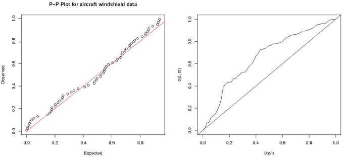
Figure 5 pp-plot and TTT plot for the aircraft windshield data.

The above data sets used for checking the suitability of proposed distribution RED along with some other distributions viz. exponentiated exponential distribution (EE) proposed by [23] , exponentiated Inverse Rayleigh distribution (EIRD) introduced by [13], type 1 half-logistic Rayleigh distribution (TIHLR) proposed [1], exponential and Lindley distribution. The ML estimates, value of -2LL, Akaike Information criteria (AIC), Corrected Akaike Information criteria (AICc), Hannan-Quinn information criterion (HQIC) are presented in the Tables 3, 5 and 7 and also K-S statistic, A-D statistic and there associated $p$-value of the considered distributions are presented in Tables 4, 6 and 8. The AIC, BIC, AICc, HQIC, K-S and A-D Statistics are computed using the following formulae:

$AIC$	$=-2LL+2k,BIC=-2LL+k\log n$
$AICc$	$=AIC+{\displaystyle \frac{2k^2+2k}{n-k-1}},HQIC=-2LL+2klog(log(n))$
$D$	$=\underset{x}{sup}|F_n(x)-F_0(x)|\mathit{\hspace{1em}}{A}^2=-N-S;$
$S$	$={\displaystyle \sum _{i=1}^N}{\displaystyle \frac{2i-1}{N}}\left[\log F(Y_i)+\log (1-F(Y_{N+1-i}))\right]$

where $k=$ the number of parameters, $n=$ the sample size, and the $F_n(x)$ is empirical distribution function $F_0(x)$ is the theoretical cumulative distribution function and $Y_i$ are the ordered data. The best distribution is the distribution corresponding to lower values of -2LL, AIC, BIC, AICc, K-S and A-D statistics and there corresponding higher $p$-values respectively.

Table 3 -2LL and information criterion for aircraft windshield data

	Estimate
Distribution	$\alpha$	$\theta$	-2LL	AIC	BIC	AICc	HQIC
RED		0.1930	212.59	214.59	216.77	214.66	215.45
EE	1.9458	0.7024	212.63	216.63	220.98	216.82	218.35
EIRD	0.2148	0.1591	322.60	326.60	330.95	326.79	328.31
TIHLR	0.5920	0.3880	215.20	219.20	223.55	219.39	220.91
Lindley		0.7543	215.32	217.32	219.49	217.38	218.17
Exponential		0.4804	225.30	227.30	229.47	227.36	228.15

Table 4 Kolmogorov-Smirnov and Anderson-Darling Statistic for aircraft windshield data

Distribution	K-S	$p$-value	A-D	$p$-value
RED	0.0719	0.8663	0.9309	0.3953
EE	0.1405	0.1397	1.3609	0.2134
EIRD	0.3639	0.0000	13.122	0.0000
TIHLR	0.1422	0.1308	2.6584	0.0411
Lindley	0.1588	0.0671	2.3349	0.0607
Exponential	0.2132	0.0045	4.1845	0.0071

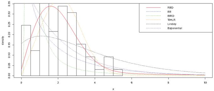
Figure 6 Fitted pdf for the aircraft windshield data.

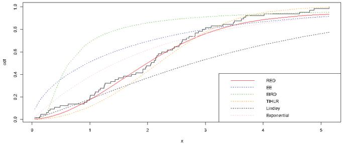
Figure 7 Fitted cdf for the aircraft windshield data.

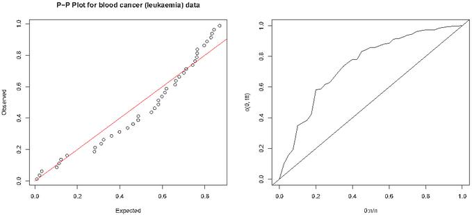
Figure 8 pp-plot and TTT plot for the blood cancer (leukaemia) data.

Table 5 -2LL and information criterion for blood cancer (leukaemia) data

	Estimate
Distribution	$\alpha$	$\theta$	-2LL	AIC	BIC	AICc	HQIC
RED		0.0839	145.35	147.35	149.04	147.46	147.96
EE	3.5189	0.6141	149.92	153.92	157.30	154.25	155.15
EIRD	0.4437	0.9562	196.05	200.05	203.43	200.37	201.27
TIHLR	0.2737	0.4364	137.41	144.79	144.79	141.73	142.63
Lindley		0.5269	160.50	162.50	164.19	162.60	163.11
Exponential		0.3184	171.56	173.56	175.24	173.67	174.17

Table 6 Kolmogorov-Smirnov and Anderson-Darling Statistic for blood cancer (leukaemia) data

Distribution	K-S	$p$-value	A-D	$p$-value
RED	0.1318	0.4903	1.1906	0.2709
EE	0.1612	0.2495	1.7137	0.1330
EIRD	0.7730	0.0000	6.3646	0.0006
TIHLR	0.1181	0.6315	0.6944	0.5625
Lindley	0.2405	0.0195	3.6452	0.0132
Exponential	0.3002	0.0015	5.4782	0.0017

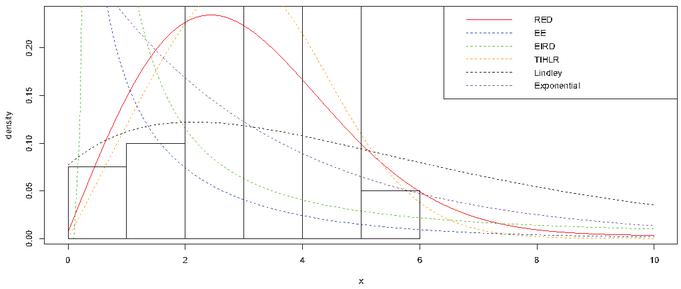
Figure 9 Fitted pdf for the blood cancer (leukaemia) data.

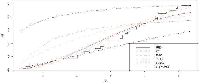
Figure 10 Fitted cdf for the blood cancer (leukaemia) data.

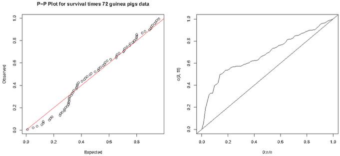
Figure 11 pp-plot and TTT plot for survival times of guinea pigs data.

Table 7 -2LL and information criterion for survival times of guinea pigs data

	Estimate
Distribution	$\alpha$	$\theta$	-2LL	AIC	BIC	AICc	HQIC
RED		0.3252	195.23	197.23	199.51	197.29	198.14
EE	3.4932	1.1181	188.95	192.95	197.51	193.13	194.77
EIRD	0.4077	0.4584	277.57	281.57	286.12	281.74	283.38
TIHLR	0.6602	0.4906	204.51	208.51	213.07	208.68	210.33
Lindley		0.8744	213.05	215.05	217.33	215.11	215.96
Exponential		0.5702	224.89	226.89	229.17	226.95	227.79

Table 8 Kolmogorov-Smirnov and Anderson-Darling Statistic survival times of guinea pigs data

Distribution	K-S	$p$-value	A-D	$p$-value
RED	0.1200	0.2508	1.0113	0.3511
EE	0.0883	0.6290	0.4572	0.7901
EIRD	0.4213	0.0000	10.437	0.0000
TIHLR	0.1866	0.0133	3.7647	0.0114
Lindley	0.1866	0.0133	3.7647	0.0114
Exponential	0.2832	0.0000	6.8837	0.0004

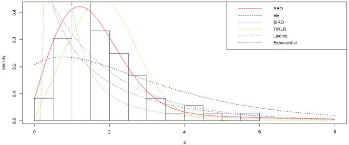
Figure 12 Fitted pdf for the survival times of guinea pigs data.

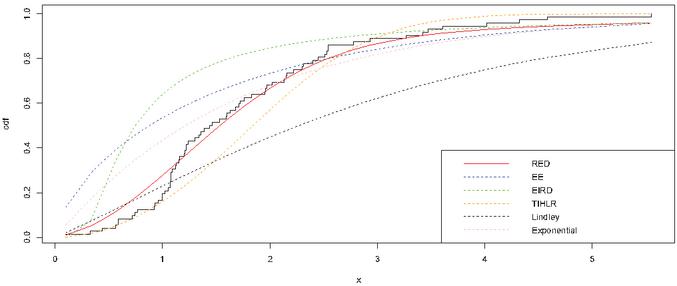
Figure 13 Fitted cdf for the survival times of guinea pigs data.

13 Conclusion

In this paper, we propose and explore the properties of the proposed distribution named as Rayleigh-Exponential Distribution (RED). We investigate some of its statistical properties like $r^{th}$ order moment, quantile function, moment generating function, characteristics function, Bonferroni, Lorenz curves, mean residual life function. Some entropy has been discussed like Rényi, Shannon entropy and cumulative residual entropy. The maximum likelihood method is employed to estimate the parameter. We fit the real data sets to demonstrate the flexibility and aptness of the proposed distribution. The RED performs better than other distributions for the first data set but in other two data set its rank is second. This shows that the RED is a competent model to some other two parameters models also. We hope that the RED distribution will attract wider application in areas such as engineering, survival and lifetime data, hydrology, economics and other areas.

Acknowledgment

Authors extend sincere thanks to the anonymous referees for their valuable suggestions to improve the quality of initial draft of the paper presented by Utpal Dhar Das in the International conference on “Recent Advances in Statistics and Data Science for Sustainable Development” in conjunction with 34th Convention of India Society for Probability and Statistics (ISPS) on 21–23rd December, 2019 in Department of Statistics, Utkal University, Bhubaneswar, Odisha.

References

[1] A. A., Albabtain. A New Extended Rayleigh Distribution, Journal of King Saud University-Science, 2576–2581, 2020.

[2] A. A., Essam, A. H., Mohamed. A weighted three-parameter Weibull distribution, J. Applied Sci. Res, 9, 6627–6635, 2013.

[3] A. Azzalini. A class of distributions which includes the normal ones, Scandinavian journal of statistics, 171–178, 1985.

[4] A. M., Abouammoh, R., Ahmad, A., Khalique. On new renewal better than used classes of life distributions, Statistics & Probability Letters, 48(2), 189–194, 2000.

[5] A., Rényi. On measures of entropy and information. In Proceedings of the Fourth Berkeley Symposium on Mathematical Statistics and Probability, Volume 1: Contributions to the Theory of Statistics. The Regents of the University of California, 1960, 547–561, 1961.

[6] Brijesh P., Singh, S., Singh, U. D., Das. A general class of new continuous mixture distribution and application. J. Math. Comput. Sci., 11(1): 585–602, 2020.

[7] Brijesh P., Singh, U. D., Das, S., Singh, A Compounded Probability Model for Decreasing Hazard and its Inferential Properties, Reliability: Theory & Applications, 16(2 (62)): 230–246, 2021.

[8] C. E., Bonferroni, Elementi di Statistica Generale. Seeber. Firenze, 1930.

[9] C. E., Shannon. A mathematical theory of communication, The Bell system technical journal, 27(3): 379–423, 1948.

[10] D.N.P., Murthy, M., Xie, R., Jiang. Weibull Models (Vol. 505), USA, John Wiley and Sons, 2004.

[11] D., Kundu, M. Z., Raqab. Generalized Rayleigh distribution: different methods of estimations, Computational statistics & data analysis, 49(1): 187–200, 2005.

[12] F., Merovci, I., Elbatal. Weibull-Rayleigh distribution: theory and applications, Appl. Math. Inf. Sci, 9(5): 1–11, 2015.

[13] G. S., Rao, S., Mbwambo. Exponentiated inverse Rayleigh distribution and an application to coating weights of iron sheets data, Journal of Probability and Statistics, 2019.

[14] H., Ahmad Sartawi, M. S., Abu-Salih. Bayesian prediction bounds for the Burr type X model, Communications in Statistics-Theory and Methods, 20(7): 2307–2330, 1991.

[15] H. J., Kim. A class of weighted multivariate normal distributions and its properties, Journal of Multivariate Analysis, 99(8): 1758–1771, 2008.

[16] J. G., Surles, W. J., Padgett. Inference for reliability and stress-strength for a scaled Burr Type X distribution, Lifetime Data Analysis, 7(2): 187–200, 2001.

[17] J. X., Kersey. Weighted inverse Weibull and beta-inverse Weibull distribution, M.Sc. Thesis, Georgia Southern University, Statesboro, Georgia, 2010.

[18] M. A., Hussian. A weighted inverted exponential distribution, International Journal of Advanced Statistics and Probability, 1(3): 142–150, 2013.

[19] M., Mahdy. A class of weighted Weibull distributions and its properties, Studies in Mathematical Sciences, 6(1): 35–45, 2013.

[20] M. Z., Raqab. Order statistics from the Burr type X model, Computers & Mathematics with Applications, 36(4): 111–120, 1998.

[21] P. E., Oguntunde, E. A., Owoloko, O. S., Balogun. On a new weighted exponential distribution: theory and application, Asian Journal of Applied Sciences, 9(1): 1–12, 2016.

[22] R.B., Wallace, D.N.P., Murthy. Reliability Wiley, New York, 2000.

[23] R. D., Gupta, D., Kundu. Exponentiated exponential family: an alternative to gamma and Weibull distributions, Biometrical Journal: Journal of Mathematical Methods in Biosciences, 43(1): 117–130, 2001.

[24] S., Nadarajah, S., Kotz. The exponentiated type distributions, Acta Applicandae Mathematica, 92(2): 97–111, 2006.

[25] S., Shahbaz, M. Q., Shahbaz, N. S., Butt. A class of weighted Weibull distribution, Pak. j. stat. oper. Res, 6(1): 53–59, 2010.

[26] T., Bjerkedal. Acquisition of Resistance in Guinea Pies infected with Different Doses of Virulent Tubercle Bacilli, American Journal of Hygiene, 72(1): 130–48, 1960.

[27] Z. F., Jaheen. Empirical Bayes estimation of the reliability and failure rate functions of the Burr type X failure model, Journal of Applied Statistical Science, 3(4): 281–288, 1996.

Biographies

Brijesh P. Singh, is currently working as Professor in the Department of Statistics, Institute of Science, Banaras Hindu University, Varanasi, India. He has obtained Ph. D. degree in Statistics from Banaras Hindu University, Varanasi and has more than 20 years’ experience of teaching and research in the area of Statistical Demography and modeling. His research interests are in statistical modeling and analysis of demographic data specially fertility, mortality, reproductive health and domestic violence with its reason and consequences.

Utpal Dhar Das, is presently working as research scholar in the Department of Statistics, Institute of Science, Banaras Hindu University, Varanasi, India. He is a bright fellow in Mathematics and Statistics and was awarded gold medal in M. Sc. (Statistics) from Assam University, Silchar. He has published 12 research articles in reputed both international and national journals. His research interests are in the areas of Generalized Probability distributions, transformed probability distributions.

Journal of Reliability and Statistical Studies, Vol. 14, Issue 2 (2021), 669–694.
doi: 10.13052/jrss0974-8024.14214
© 2021 River Publishers