Reliability Test Plan Based on Logistic-Exponential Distribution and Its Application

Abhimanyu Singh Yadav¹, Mahendra Saha², Shivanshi Shukla^2,* Harsh Tripathi^{2, 3} and Rajashree Dey²

¹Department of Statistics, Banaras Hindu University, India

²Department of Statistics, Central University of Rajasthan, Rajasthan,

India

³Department of Mathematics, Lovely Professional University, Punjab, India

E-mail: speak2shivanshi@gmail.com

*Corresponding Author

Received 02 February 2021; Accepted 23 November 2021; Publication 14 December 2021

Abstract

In this article, a reliability test plan is developed for Logistic-exponential distribution (LoED) under time truncated life test scheme. The distribution has been chosen because it can used to model lifetime of several reliability phenomenon and it performs better than many well known existing distributions. With the discussions of statistical properties of the aforesaid model, the reliability test plan has been established under the assumption of median quality characteristics when minimum confidence level $P^{*}$ is given. To quench the objective of the paper i.e; to serve as a guiding aid to the emerging practitioners, minimum sample sizes have been obtained by using binomial approximation and Poisson approximation for the proposed plan. Further, operating characteristic (OC) values for the various choices of quality level are placed. Also, minimum ratio of true median life to specified life has been presented for specified producer’s risk. Important findings of the proposed reliability test plan are given for considered value of $k=0.75,1,2$. To demonstrate the appropriateness of suggested reliability test plan is achieved using four real life situation.

Keywords: Consumer’s risk, logistic-exponential distribution, operating characteristic curve, producer’s risk, reliability life test, termination ratio.

1 Introduction

Lifetime of products follow a specific behaviour that is described by probability distribution. Estimation and inferential part of the developed theory of statistics are the key interest of the researcher and this is fulfil with the help of these distributions. Thus, for our study we have used a statistical distribution, LoED [see, Lan and Leemis ($2008$)]. The LoED encircle four shapes: increasing failure rate, decreasing failure rate, bathtub-shaped failure rate and upside-down bathtub-shaped failure rate. Such shapes are easily observable in daily life phenomena (for the more detail of LoED, readers may refer to Lan and Leemis ($2008$)). Plethora of shape choices for the event make the LoED special over the other distributions model. Flexibility of LoED encourages to researchers for evolution of various versions of LoED and some of them are: Mashail M. Al Sobhi ($2020$), Ali et al. ($2020$) and Elgarhy et al. ($2020$) have developed Inverse-Power LoED, Two-Parameter LoED and Type II Half LoED, respectively. For $k=1$, LoED coincide with exponential distribution thus, exponential distribution is a special case of LoED. Therefore, keeping in mind the utility of the aforesaid distribution we desire to present a related reliability test plan. The probability density function (PDF) and cumulative distribution function (CDF) of LoED are given as;

$$f(x)=\frac{\lambda k{(e^{\lambda x}-1)}^{(k-1)}{e}^{\lambda x}}{{(1+{(e^{\lambda x}-1)}^k)}^2}$$

(1)

and

$F(x)={\displaystyle \frac{{(e^{\lambda x}-1)}^k}{1+{(e^{\lambda x}-1)}^k}}$

(2)

respectively. The $p-th$ fractile of LoED is given as;

$$x_p=\frac{1}{\lambda }\log \left(1+{\left(\frac{p}{1-p}\right)}^{1/k}\right)$$

(3)

Putting $p=\frac{1}{2}$ in Equation (3), we get the median of the LoED and the expression of median for considered probability distribution model is:

$$x_{1/2}=\frac{1}{\lambda }\log (2)=Med$$

(4)

Statistical Quality Control (SQC) is enriched with the techniques of controlling quality and two important element of this technique are statistical process control and the statistical product control. For the establishment of proposed reliability test plan, we used technique of statistical product control, acceptance sampling plan. Acceptance sampling plan is a gateway for the acceptance/rejection decision to be taken for the lot of products subjected to inspection. In this course of decision making we are likely to commit two types of error; accepting the bad lot and rejecting the good lot popularly termed as consumer’s risk and producer’s risk respectively. If lifetime of items are the basis for making decision, such a plan is named reliability test plan.

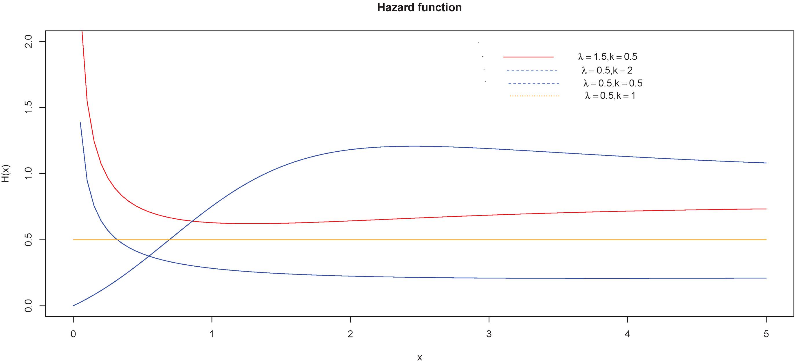
Figure 1 HRF of LoED.

Major contributions of this paper are:

1. First is to established the reliability test plan for LoED and all the tables of the proposed plan viz., sample sizes, OC value and minimum ratio of $Med/Me{d}_0$.

2. Second is to illustrate the application of this plan in real life situations.

Rest of article is organized as follows: In Section 2, we described the reliability test plan and mention the works which are done by many authors. Description of Tables and findings for the proposed reliability test plan have been given in Section 3. Applications to failure data are given in Section 4. Conclusions of the suggested reliability test plan are given in Section 5.

2 Reliability Test Plan

Reliability test plan is applicable in those area in which experimenter takes the decision regrading the quality of products (or lot of product) based on the testing of the some units of the lot and this can be done by using life testing experiment. Life testing is the integral part of the experiment because it emphasis on the reliability or quality of the products. $100$ percent inspection of the whole lot is not possible in real life due to several issues such as cost of experiment, manpower and time of experiment e.t.c. To overcome these mentioned situations or difficulties, time truncated life testing experiment is a good alternative to usual life testing experiment. Thus, a fixed number of items or products are drawn from the given lot randomly and are tested under the considered assumptions for a prefixed time. Based on this time truncated life test of items, experimenter (or producer or consumer) could pass a judgement on the reliability or quality of lot which is of the deep interest to the experimenter for the acceptance and rejection of lot. Conventionally, the attribute of product that is inspected is lifetime of the item. Therefore, after the due inspection procedure what we gather is the lifetimes of the sample selected from the lot of product and having obtained the median lifetime of the sample, we test it against specified minimum median lifetime we desire. Median lifetime is generally preferred in the cases when the lifetimes follow the skewed probability distribution. Criteria of acceptance or rejection of the lot depends on median lifetime, i.e., if the true median lifetime exceeds or equal the specified minimum median lifetime then accept the lot , otherwise reject the lot. More specifically, we wish to set the lower confidence limit on the median life of the sample. Standard procedure to achieve the objective regarding the lot acceptance or rejection is to observe the number of defective items from the selected sample till the prefixed truncated time and if it exceeds the acceptance number ‘$c$’ (say), we reject the lot, otherwise accept it. It is to be noted that test stands terminated with the decision of rejection if one observes the failures exceeding ‘$c$’ before decided time ‘$t$’. In such a truncated life test, our interest lies in obtaining the smallest sample size to arrive at a decision.

Several authors have contributed in the development of reliability test plan. Goode and Kao (1961) threw some light on acceptance sampling plan for weibull distribution. Acceptance sampling based on life tests for gamma distribution was proposed by Gupta et al. (1961). Similar plan has been developed by Kantam et al. (2001) for log-logistic model while Rosaiah et al. (2005) discussed similar problem for inverse rayleigh distribution distribution. Gupta et al. (2010) introduced the estimation of reliability for Marshall-Olkin extended Lomax distributions. In 2006, Rosaiah et al. discussed the acceptance sampling based on truncated life tests for Pareto distribution. Rao (2009) discussed reliability test plan for Marshall-Olkin extended exponential distribution. Krishna et al. (2013) not only introduced the Marshall-Olkin Frećhet distribution but also discussed its applications in reliability and sampling plans. Jose et al. (2015) discussed reliability test plan for the negative binomial extreme stable Marshall-Olkin Pareto distribution. Recently, Jose et al. (2018) introduced the reliability test plan for the Gumbel-Uniform Distribution. Gillariose and Tomy (2021), Ravikumar et al. (2019), Rosaiah et al. (2017) and Kaviayarasu and Fawaz (2017) have developed reliability sampling plan for Birnbaum-Saunders distribution, Burr type X distribution, Odds exponential log-logistic distribution and Weibull Poisson distribution, respectively.

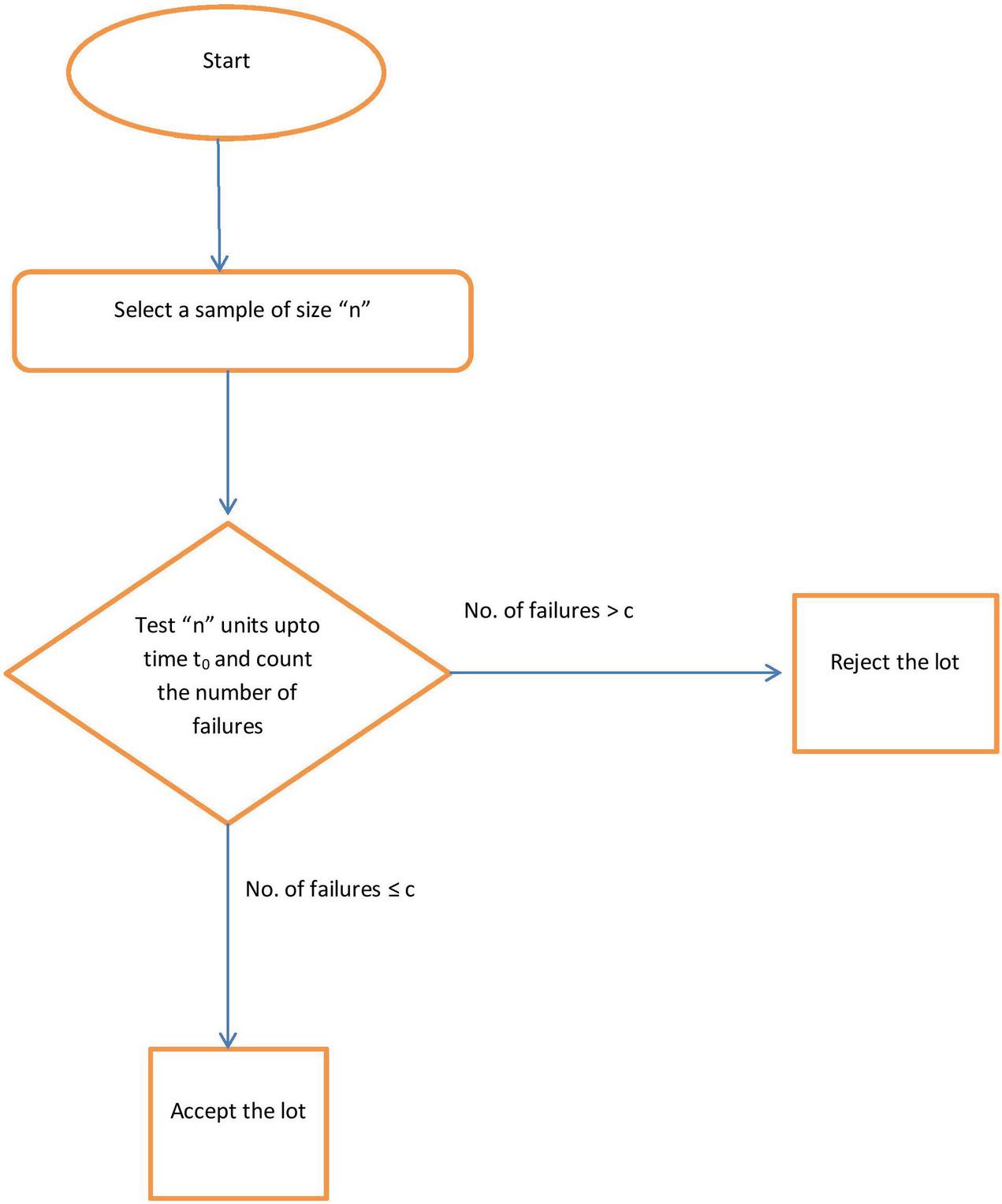
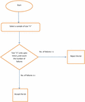
In this article we suggested a reliability test plan for the lot of products whose lifetimes are governed by LoED. Median is good measure quality characteristic in case of skewed data thus we make our decision based on median life of items. Therefore considered distribution LoED is skewed. Further it is assumed that the distribution shape parameter $k$ is known, while scale parameter $\lambda$ is unknown. Here lifetime of the product depends only on $\lambda$ and it can be easily perceived that the median of LoED depends on $\lambda$. $F(t_0)$ CDF of LoED can be written in the form of median $(Med)$ and also easily converted in the form of $t_0/Me{d}_0$. Figure 2 represents the flowchart of reliability test plan.

Figure 2 Flowchart of reliability test plan.

Notationally a sampling plan exhibits the following;

• number of units put on test: n

• acceptance number: c

• pre-specified test time: $t_0$

• ratio $\frac{t_0}{Me{d}_0}$ where $Me{d}_0$ is specified value of median

Consumer’s risk which is the probability of accepting a bad lot not to exceed $1-P^{*}$ where $P^{*}$ is minimum confidence level that should possess in order to be accepted by the decision procedure. Decision of acceptance of lot for the proposed problem implies that the true median life exceeds minimum required median life. For fixed $P^{*}$, our plan is characterized as $(n,c,\frac{t_0}{Me{d}_0})$. To validate the applicability of Binomial distribution we consider lot of large size. Here $L(p_0)$ is the OC function [see, Equation (5)] of the plan, given as.

$$L(p_0)=\sum _{i=0}^c\left(\genfrac{}{}{0pt}{}{n}{i}\right)p_0{}^{i}1-p_0{}^{n-i}$$

(5)

where:

$$p_0=\frac{{\{e^{\left(\frac{t_0}{Me{d}_0}\frac{Med}{Me{d}_0}\log 2\right)}-1\}}^k}{1+{\{e^{\left(\frac{t_0}{Me{d}_0}\frac{Med}{Me{d}_0}\log 2\right)}-1\}}^k}$$

The objective is to determine smallest sample size to make a decision for given $P^{*}$, $t_0/Me{d}_0$ and $c$ such that;

$$\sum _{i=0}^c\left(\genfrac{}{}{0pt}{}{n}{i}\right)p_0{}^{i}1-p_0{}^{n-i}\le 1-P^{*}$$

(6)

It can be seen that probability of failure before time ‘$t_0$’ depends only on ratio $\frac{t_0}{Me{d}_0}$.

The least possible value of n under the condition that Equation 6 holds are arranged in Tables 1, 5, 9 for $k=0.75,1,2$. Assume that the value of $P^{*}=0.75$, 0.90, 0.95, 0.99, $t_0/Me{d}_0=0.241$, 0.361, 0.482, 0.602, 0.903, 1.204, 1.505, 1.806, 2.206 and $k=0.75,1,2$.

If $p_0=F(t_0;k,\lambda )$ is small and n is large, Poisson probability can be taken as approximation for Binomial probability with parameter $\lambda =n{p}_0$ so that the left side of Equation (6) can be written as

$$L^{*}(p_0)=\sum _{i=0}^c\frac{{\lambda }^i}{i!}{e}^{-\lambda }\le 1-P^{*}$$

(7)

The minimum n satisfying Equation (7) for same values of $P^{*}$ and $t_0/Me{d}_0$ as used for Equation (6) are presented in Tables 2, 6, 10. Now OC function in case of Poisson probability is given in Equation (8):

$$L^{*}(p_0)=\sum _{i=0}^c\frac{{\lambda }^i}{i!}{e}^{-\lambda }$$

(8)

Tables 3, 7, 11 provide the OC values through OC function which depends upon $Med/Me{d}_0$ for some specified sampling plan $(n,c,t_0/Me{d}_0)$.

Producers risk is the probability of rejecting a lot and obtained by using OC function, it can be obtained as

$$L(p_0)=L[F(t_0;k,\lambda )]$$

(9)

For a given sampling plan $(n,c,t_0/Me{d}_0)$ and specified producer’s risk is $0.05$. It is of interest to know for what value of $Med/Me{d}_0$, producer’s risk will be less than or equal to $0.05$. This is achieved when the following is satisfied;

$$\sum _{i=0}^c\left(\genfrac{}{}{0pt}{}{n}{i}\right)p_0{}^i(1-p_0{}^{n-i})\ge 0.95$$

(10)

The minimum value of $Med/Me{d}_0$ satisfying Equation 10 thus obtained for same sampling plans are displayed in Tables 4, 8, 12.

3 Description of the Tables and Findings

Assume that the lifetime of items follow the LoED with known parameter $k=0.75,1,2$. All computed values of proposed reliability test plan are placed in Tables 1–12 for $k=0.75,1,2$. To understand the Tables for all considered value of $k$, first we explain the results for $k=0.75$. Suppose the true unknown median life to be at least 1000 hours with confidence $P^{*}=0.75$ and decides to stop the test at $t=482$ hours. Further, if we take acceptance number $c=2$, then evidently from table $n$, the smallest sample size is $11$. What we have observed is that if till $482$ hours in a sample of size $11$, not more than two failures are spotted then the experimenter firmly asserts with $75$ percent confidence that median life of the lot is at least $1000$ hours. In Poisson set up same can be asserted for $n=56$. For sampling plan $(n=12,c=2,t_0/Me{d}_0=0.482)$ and confidence level $P^{*}=0.75$ under LoED with $k=0.75$, the values of operating characteristic function as seen from Table 3 for considered value of $k=0.75$ is;

$Med/Me{d}_0$	2	4	6	8	10	12
$L(p_0)$	$0.558$	$0.814$	$0.899$	$0.938$	$0.958$	$0.970$

Table 1 Minimum sample size for the specified ratio $t_0/Me{d}_0$, confidence level $P^{*}$, acceptance number $c$ and $k=0.75$ by using binomial approximation

		$t_0/Me{d}_0$
$P^{*}$	$c$	$0.482$	$0.602$	$0.903$	$1.204$	$1.505$	$1.806$	$2.206$
$0.75$	$0$	$4$	$3$	$3$	$2$	$2$	$2$	$2$
	$1$	$8$	$7$	$5$	$4$	$4$	$4$	$3$
	$2$	$11$	$10$	$8$	$7$	$6$	$5$	$5$
	$3$	$15$	$13$	$10$	$9$	$8$	$7$	$6$
	$4$	$18$	$16$	$12$	$11$	$9$	$9$	$8$
	$5$	$21$	$19$	$15$	$13$	$11$	$10$	$9$
	$6$	$25$	$22$	$17$	$15$	$13$	$12$	$11$
	$7$	$28$	$25$	$19$	$17$	$15$	$13$	$12$
	$8$	$31$	$27$	$22$	$19$	$17$	$15$	$14$
	$9$	$35$	$30$	$24$	$21$	$18$	$17$	$15$
	$10$	$38$	$33$	$26$	$22$	$20$	$18$	$17$
$0.90$	$0$	$6$	$5$	$4$	$3$	$3$	$3$	$2$
	$1$	$11$	$9$	$7$	$6$	$5$	$5$	$4$
	$2$	$15$	$13$	$10$	$8$	$7$	$7$	$6$
	$3$	$19$	$16$	$13$	$11$	$9$	$8$	$7$
	$4$	$22$	$19$	$15$	$13$	$11$	$10$	$9$
	$5$	$26$	$23$	$18$	$15$	$13$	$12$	$11$
	$6$	$30$	$26$	$20$	$17$	$15$	$14$	$12$
	$7$	$33$	$29$	$23$	$19$	$17$	$15$	$14$
	$8$	$37$	$32$	$25$	$21$	$19$	$17$	$15$
	$9$	$40$	$35$	$28$	$23$	$21$	$19$	$17$
	$10$	$44$	$38$	$30$	$25$	$22$	$20$	$18$
$0.95$	$0$	$8$	$7$	$5$	$4$	$4$	$3$	$3$
	$1$	$13$	$11$	$8$	$7$	$6$	$5$	$5$
	$2$	$17$	$15$	$11$	$10$	$8$	$7$	$7$
	$3$	$21$	$18$	$14$	$12$	$10$	$9$	$8$
	$4$	$25$	$22$	$17$	$14$	$12$	$11$	$10$
	$5$	$29$	$25$	$20$	$16$	$14$	$13$	$12$
	$6$	$33$	$29$	$22$	$19$	$16$	$15$	$13$
	$7$	$37$	$32$	$25$	$21$	$18$	$17$	$15$
	$8$	$40$	$35$	$27$	$23$	$20$	$18$	$16$
	$9$	$44$	$38$	$30$	$25$	$22$	$20$	$18$
	$10$	$48$	$41$	$32$	$27$	$24$	$22$	$20$
$0.99$	$0$	$12$	$10$	$8$	$6$	$5$	$5$	$4$
	$1$	$17$	$15$	$11$	$9$	$8$	$7$	$6$
	$2$	$22$	$19$	$15$	$12$	$10$	$9$	$8$
	$3$	$27$	$23$	$18$	$15$	$13$	$11$	$10$
	$4$	$31$	$27$	$21$	$17$	$15$	$13$	$12$
	$5$	$35$	$31$	$24$	$20$	$17$	$15$	$14$
	$6$	$40$	$34$	$26$	$22$	$19$	$17$	$15$
	$7$	$44$	$38$	$29$	$24$	$21$	$19$	$17$
	$8$	$48$	$41$	$32$	$27$	$23$	$21$	$19$
	$9$	$52$	$45$	$35$	$29$	$25$	$23$	$20$
	$10$	$55$	$48$	$37$	$31$	$27$	$25$	$22$

Table 2 Minimum sample size for the specified ratio $t_0/Me{d}_0$, confidence level $P^{*}$, acceptance number $c$ and $k=0.75$ by using poisson approximation

		$t_0/Me{d}_0$
$P^{*}$	$c$	$0.482$	$0.602$	$0.903$	$1.204$	$1.505$	$1.806$	$2.206$
$0.75$	$0$	$5$	$4$	$3$	$3$	$3$	$3$	$2$
	$1$	$9$	$8$	$6$	$5$	$5$	$5$	$4$
	$2$	$12$	$11$	$9$	$8$	$7$	$6$	$6$
	$3$	$16$	$14$	$11$	$10$	$9$	$8$	$8$
	$4$	$19$	$17$	$14$	$12$	$11$	$10$	$9$
	$5$	$23$	$20$	$16$	$14$	$13$	$12$	$11$
	$6$	$26$	$23$	$19$	$16$	$14$	$13$	$12$
	$7$	$30$	$26$	$21$	$18$	$16$	$15$	$14$
	$8$	$33$	$29$	$23$	$20$	$18$	$17$	$15$
	$9$	$36$	$32$	$26$	$22$	$20$	$18$	$17$
	$10$	$40$	$35$	$28$	$24$	$22$	$20$	$18$
$0.90$	$0$	$7$	$7$	$5$	$5$	$4$	$4$	$4$
	$1$	$12$	$11$	$9$	$8$	$7$	$6$	$6$
	$2$	$16$	$15$	$12$	$10$	$9$	$9$	$8$
	$3$	$21$	$18$	$15$	$13$	$11$	$11$	$10$
	$4$	$24$	$22$	$17$	$15$	$14$	$13$	$12$
	$5$	$28$	$25$	$20$	$17$	$16$	$14$	$13$
	$6$	$32$	$28$	$23$	$20$	$18$	$16$	$15$
	$7$	$36$	$32$	$25$	$22$	$20$	$18$	$17$
	$8$	$39$	$35$	$28$	$24$	$22$	$20$	$18$
	$9$	$43$	$38$	$30$	$26$	$24$	$22$	$20$
	$10$	$47$	$41$	$33$	$29$	$26$	$24$	$22$
$0.95$	$0$	$9$	$8$	$7$	$6$	$5$	$5$	$5$
	$1$	$15$	$13$	$11$	$9$	$8$	$8$	$7$
	$2$	$19$	$17$	$14$	$12$	$11$	$10$	$9$
	$3$	$24$	$21$	$17$	$15$	$13$	$12$	$11$
	$4$	$28$	$25$	$20$	$17$	$15$	$14$	$13$
	$5$	$32$	$28$	$23$	$20$	$18$	$16$	$15$
	$6$	$36$	$32$	$25$	$22$	$20$	$18$	$17$
	$7$	$40$	$35$	$28$	$24$	$22$	$20$	$19$
	$8$	$44$	$39$	$31$	$27$	$24$	$22$	$20$
	$9$	$48$	$42$	$34$	$29$	$26$	$24$	$22$
	$10$	$51$	$45$	$36$	$31$	$28$	$26$	$24$
$0.99$	$0$	$14$	$13$	$10$	$9$	$8$	$7$	$7$
	$1$	$20$	$18$	$15$	$13$	$11$	$10$	$10$
	$2$	$26$	$23$	$18$	$16$	$14$	$13$	$12$
	$3$	$31$	$27$	$22$	$19$	$17$	$16$	$14$
	$4$	$35$	$31$	$25$	$22$	$19$	$18$	$17$
	$5$	$40$	$35$	$28$	$24$	$22$	$20$	$19$
	$6$	$44$	$39$	$31$	$27$	$24$	$22$	$21$
	$7$	$49$	$43$	$34$	$30$	$27$	$25$	$23$
	$8$	$53$	$46$	$37$	$32$	$29$	$27$	$25$
	$9$	$57$	$50$	$40$	$35$	$31$	$29$	$26$
	$10$	$61$	$54$	$43$	$37$	$33$	$31$	$28$

Table 3 Values of the operating characteristic function of the sampling plan ($n,c,t_0/Me{d}_0$) for given confidence level $p*$ with $k=0.75$ for $c=2$

				$Med/Me{d}_0$
$p*$	$n$	$c$	$t_0/Me{d}_0$	$2$	$4$	$6$	$8$	$10$	$12$
$0.75$	$11$	$2$	$0.482$	$0.558$	$0.814$	$0.899$	$0.938$	$0.958$	$0.970$
$0.75$	$10$	$2$	$0.602$	$0.524$	$0.793$	$0.887$	$0.929$	$0.952$	$0.965$
$0.75$	$8$	$2$	$0.903$	$0.499$	$0.777$	$0.877$	$0.922$	$0.947$	$0.962$
$0.75$	$7$	$2$	$1.204$	$0.466$	$0.755$	$0.863$	$0.913$	$0.940$	$0.956$
$0.75$	$6$	$2$	$1.505$	$0.483$	$0.767$	$0.870$	$0.918$	$0.944$	$0.959$
$0.75$	$5$	$2$	$1.806$	$0.589$	$0.808$	$0.896$	$0.935$	$0.956$	$0.968$
$0.75$	$5$	$2$	$2.206$	$0.452$	$0.748$	$0.858$	$0.909$	$0.937$	$0.954$
$0.90$	$15$	$2$	$0.482$	$0.334$	$0.656$	$0.797$	$0.868$	$0.907$	$0.932$
$0.90$	$13$	$2$	$0.602$	$0.331$	$0.652$	$0.794$	$0.866$	$0.906$	$0.930$
$0.90$	$10$	$2$	$0.903$	$0.330$	$0.651$	$0.792$	$0.864$	$0.904$	$0.929$
$0.90$	$8$	$2$	$1.204$	$0.361$	$0.677$	$0.811$	$0.877$	$0.914$	$0.936$
$0.90$	$7$	$2$	$1.505$	$0.357$	$0.765$	$0.809$	$0.876$	$0.913$	$0.936$
$0.90$	$7$	$2$	$1.806$	$0.271$	$0.599$	$0.755$	$0.836$	$0.883$	$0.913$
$0.90$	$6$	$2$	$2.206$	$0.297$	$0.626$	$0.774$	$0.850$	$0.893$	$0.921$
$0.95$	$17$	$2$	$0.482$	$0.250$	$0.576$	$0.739$	$0.825$	$0.876$	$0.907$
$0.95$	$15$	$2$	$0.602$	$0.235$	$0.559$	$0.726$	$0.815$	$0.868$	$0.901$
$0.95$	$11$	$2$	$0.903$	$0.262$	$0.588$	$0.747$	$0.831$	$0.879$	$0.910$
$0.95$	$10$	$2$	$1.204$	$0.203$	$0.524$	$0.697$	$0.793$	$0.850$	$0.887$
$0.95$	$8$	$2$	$1.505$	$0.257$	$0.584$	$0.743$	$0.827$	$0.877$	$0.908$
$0.95$	$7$	$2$	$1.806$	$0.271$	$0.549$	$0.755$	$0.836$	$0.883$	$0.913$
$0.95$	$7$	$2$	$2.206$	$0.186$	$0.508$	$0.684$	$0.782$	$0.842$	$0.880$
$0.99$	$22$	$2$	$0.482$	$0.112$	$0.379$	$0.590$	$0.708$	$0.784$	$0.834$
$0.99$	$19$	$2$	$0.602$	$0.110$	$0.393$	$0.586$	$0.704$	$0.780$	$0.831$
$0.99$	$15$	$2$	$0.903$	$0.095$	$0.365$	$0.559$	$0.682$	$0.761$	$0.815$
$0.99$	$12$	$2$	$1.204$	$0.108$	$0.389$	$0.581$	$0.699$	$0.776$	$0.827$
$0.99$	$10$	$2$	$1.505$	$0.124$	$0.417$	$0.606$	$0.721$	$0.792$	$0.841$
$0.99$	$9$	$2$	$1.806$	$0.118$	$0.409$	$0.599$	$0.714$	$0.787$	$0.836$
$0.99$	$8$	$2$	$2.206$	$0.113$	$0.403$	$0.594$	$0.710$	$0.784$	$0.833$

Table 4 Minimum ratio of true $Med$ and required $Me{d}_0$ for the acceptability of a lot with producer’s risk of 0.05 for $k=0.75$

		$Med/Me{d}_0$
$p*$	$c$	$0.482$	$0.602$	$0.903$	$1.204$	$1.505$	$1.806$	$2.206$
$0.75$	$0$	$110.53$	$93.87$	$140.8$	$108.89$	$136.11$	$163.33$	$199.51$
$0.75$	$1$	$18.99$	$19.51$	$17.67$	$16.61$	$20.76$	$24.91$	$18.88$
$0.75$	$2$	$9.03$	$9.76$	$10.33$	$11.1$	$10.72$	$9.33$	$11.39$
$0.75$	$3$	$6.75$	$6.75$	$6.63$	$7.41$	$7.55$	$7.11$	$6.45$
$0.75$	$4$	$5.15$	$5.34$	$4.99$	$5.73$	$4.98$	$5.97$	$5.81$
$0.75$	$5$	$4.26$	$4.54$	$4.61$	$4.79$	$4.40$	$4.39$	$4.32$
$0.75$	$6$	$3.95$	$4.02$	$3.92$	$4.19$	$4.01$	$4.12$	$4.22$
$0.75$	$7$	$3.51$	$3.66$	$3.45$	$3.77$	$3.73$	$3.37$	$3.48$
$0.75$	$8$	$3.20$	$3.19$	$3.38$	$3.47$	$3.52$	$3.29$	$3.48$
$0.75$	$9$	$3.10$	$3.01$	$3.09$	$3.23$	$3.01$	$3.22$	$3.02$
$0.75$	$10$	$2.89$	$2.87$	$2.86$	$2.81$	$2.92$	$2.83$	$3.06$
$0.90$	$0$	$190.21$	$186.13$	$207.08$	$187.74$	$234.63$	$281.60$	$199.51$
$0.90$	$1$	$29.96$	$28.1$	$29.27$	$31.05$	$29.44$	$35.33$	$30.43$
$0.90$	$2$	$14.31$	$14.48$	$14.63$	$13.77$	$13.87$	$16.64$	$15.71$
$0.90$	$3$	$9.64$	$9.3$	$10.12$	$10.34$	$9.26$	$9.06$	$8.68$
$0.90$	$4$	$7.01$	$7.00$	$7.23$	$7.62$	$7.16$	$7.25$	$7.29$
$0.90$	$5$	$5.94$	$6.14$	$6.24$	$6.14$	$5.98$	$6.21$	$6.45$
$0.90$	$6$	$5.25$	$5.25$	$5.16$	$5.22$	$5.23$	$5.53$	$5.03$
$0.90$	$7$	$4.55$	$4.64$	$4.78$	$4.60$	$4.71$	$4.48$	$4.78$
$0.90$	$8$	$4.23$	$4.20$	$4.21$	$4.15$	$4.33$	$4.22$	$4.02$
$0.90$	$9$	$3.83$	$3.87$	$4.02$	$3.81$	$4.04$	$4.02$	$3.94$
$0.90$	$10$	$3.65$	$3.61$	$3.67$	$3.55$	$3.51$	$3.50$	$3.46$
$0.95$	$0$	$279.46$	$291.97$	$279.2$	$276.1$	$345.12$	$281.6$	$343.97$
$0.95$	$1$	$37.91$	$37.41$	$35.56$	$39.02$	$38.81$	$35.33$	$43.16$
$0.95$	$2$	$17.16$	$17.87$	$16.92$	$19.51$	$17.21$	$16.64$	$20.33$
$0.95$	$3$	$11.17$	$11.10$	$11.36$	$11.89$	$11.05$	$11.11$	$11.06$
$0.95$	$4$	$8.5$	$8.76$	$8.82$	$8.61$	$8.32$	$8.59$	$8.86$
$0.95$	$5$	$7.01$	$6.98$	$7.39$	$6.85$	$6.81$	$7.18$	$7.59$
$0.95$	$6$	$6.07$	$6.22$	$6.03$	$6.31$	$5.87$	$6.28$	$5.88$
$0.95$	$7$	$5.42$	$5.42$	$5.48$	$5.47$	$5.22$	$5.65$	$5.47$
$0.95$	$8$	$4.77$	$4.84$	$4.78$	$4.87$	$4.75$	$4.70$	$4.58$
$0.95$	$9$	$4.44$	$4.41$	$4.52$	$4.82$	$4.40$	$4.43$	$4.42$
$0.95$	$10$	$4.18$	$4.08$	$4.09$	$4.07$	$4.12$	$4.21$	$4.28$
$0.99$	$0$	$480.42$	$470.31$	$523.55$	$475.13$	$465.33$	$558.39$	$505.87$
$0.99$	$1$	$55.09$	$57.83$	$56.12$	$56.20$	$59.27$	$58.53$	$56.88$
$0.99$	$2$	$24.81$	$25.14$	$26.8$	$25.71$	$24.38$	$24.86$	$25.23$
$0.99$	$3$	$16.1$	$15.94$	$16.65$	$16.85$	$16.87$	$15.51$	$16.20$
$0.99$	$4$	$11.66$	$11.89$	$12.24$	$11.76$	$12.04$	$11.43$	$12.29$
$0.99$	$5$	$9.27$	$9.67$	$9.84$	$9.85$	$9.46$	$9.21$	$9.99$
$0.99$	$6$	$8.09$	$7.93$	$7.87$	$8.03$	$7.88$	$7.83$	$7.66$
$0.99$	$7$	$7.04$	$7.05$	$6.96$	$6.83$	$6.83$	$6.89$	$6.90$
$0.99$	$8$	$6.29$	$6.19$	$6.30$	$6.38$	$6.08$	$6.22$	$6.35$
$0.99$	$9$	$5.73$	$5.74$	$5.81$	$5.69$	$5.52$	$5.72$	$5.41$
$0.99$	$10$	$5.15$	$5.22$	$5.19$	$5.16$	$5.09$	$5.33$	$5.14$

Table 5 Minimum sample size for the specified ratio $t_0/Me{d}_0$, confidence level $P^{*}$, acceptance number $c$ and $k=1$ by using binomial approximation

		$t_0/Me{d}_0$
$P^{*}$	$c$	$0.482$	$0.602$	$0.903$	$1.204$	$1.505$	$1.806$	$2.206$
$0.75$	$0$	$5$	$4$	$3$	$2$	$2$	$2$	$1$
	$1$	$9$	$7$	$5$	$4$	$4$	$3$	$3$
	$2$	$13$	$11$	$8$	$6$	$5$	$5$	$4$
	$3$	$17$	$14$	$10$	$8$	$7$	$6$	$6$
	$4$	$21$	$18$	$13$	$10$	$9$	$8$	$7$
	$5$	$25$	$21$	$15$	$12$	$11$	$9$	$8$
	$6$	$29$	$24$	$17$	$14$	$12$	$11$	$10$
	$7$	$33$	$27$	$20$	$16$	$14$	$12$	$11$
	$8$	$37$	$31$	$22$	$18$	$16$	$14$	$13$
	$9$	$41$	$34$	$24$	$20$	$17$	$15$	$14$
	$10$	$45$	$37$	$27$	$22$	$19$	$17$	$15$
$0.90$	$0$	$7$	$16$	$4$	$3$	$3$	$2$	$2$
	$1$	$13$	$10$	$7$	$6$	$5$	$4$	$4$
	$2$	$17$	$14$	$10$	$8$	$7$	$6$	$5$
	$3$	$22$	$18$	$13$	$10$	$9$	$8$	$7$
	$4$	$27$	$22$	$15$	$12$	$10$	$9$	$8$
	$5$	$31$	$25$	$18$	$14$	$12$	$11$	$10$
	$6$	$35$	$29$	$21$	$16$	$14$	$12$	$11$
	$7$	$39$	$32$	$23$	$19$	$16$	$14$	$12$
	$8$	$44$	$36$	$26$	$21$	$18$	$16$	$14$
	$9$	$48$	$39$	$28$	$23$	$19$	$17$	$15$
	$10$	$52$	$43$	$31$	$25$	$21$	$19$	$17$
$0.95$	$0$	$9$	$8$	$5$	$4$	$3$	$2$	$2$
	$1$	$15$	$12$	$9$	$7$	$6$	$5$	$4$
	$2$	$20$	$17$	$12$	$9$	$8$	$7$	$6$
	$3$	$25$	$21$	$15$	$11$	$10$	$8$	$7$
	$4$	$30$	$25$	$17$	$14$	$12$	$10$	$9$
	$5$	$35$	$28$	$20$	$16$	$13$	$12$	$10$
	$6$	$39$	$32$	$23$	$18$	$15$	$13$	$12$
	$7$	$44$	$36$	$25$	$20$	$17$	$15$	$13$
	$8$	$48$	$39$	$28$	$22$	$19$	$17$	$15$
	$9$	$52$	$43$	$30$	$24$	$21$	$18$	$16$
	$10$	$57$	$46$	$33$	$26$	$22$	$20$	$18$
$0.99$	$0$	$14$	$12$	$8$	$6$	$5$	$4$	$4$
	$1$	$21$	$17$	$12$	$9$	$7$	$6$	$5$
	$2$	$27$	$22$	$15$	$12$	$10$	$8$	$7$
	$3$	$32$	$26$	$18$	$14$	$12$	$10$	$9$
	$4$	$37$	$30$	$21$	$17$	$14$	$12$	$10$
	$5$	$42$	$35$	$24$	$19$	$16$	$14$	$12$
	$6$	$47$	$39$	$27$	$21$	$18$	$16$	$14$
	$7$	$52$	$43$	$30$	$24$	$20$	$17$	$15$
	$8$	$57$	$46$	$33$	$26$	$22$	$19$	$17$
	$9$	$61$	$50$	$35$	$28$	$24$	$21$	$18$
	$10$	$66$	$54$	$38$	$30$	$25$	$22$	$20$

Table 6 Minimum sample size for the specified ratio $t_0/Me{d}_0$, confidence level $P^{*}$, acceptance number $c$ and $k=1$ by using poisson approximation

$t_0/Me{d}_0$
$P^{*}$	$c$	$0.482$	$0.602$	$0.903$	$1.204$	$1.505$	$1.806$	$2.206$
$0.75$	$0$	$6$	$5$	$3$	$3$	$3$	$2$	$2$
	$1$	$10$	$8$	$6$	$5$	$5$	$4$	$4$
	$2$	$14$	$12$	$9$	$7$	$7$	$6$	$6$
	$3$	$18$	$15$	$11$	$10$	$8$	$8$	$7$
	$4$	$23$	$19$	$14$	$12$	$10$	$9$	$9$
	$5$	$27$	$22$	$16$	$14$	$12$	$11$	$10$
	$6$	$31$	$26$	$19$	$16$	$14$	$12$	$11$
	$7$	$35$	$29$	$21$	$18$	$15$	$14$	$13$
	$8$	$39$	$32$	$24$	$20$	$17$	$16$	$14$
	$9$	$42$	$35$	$26$	$22$	$19$	$18$	$16$
	$10$	$46$	$39$	$28$	$24$	$21$	$19$	$17$
$0.90$	$0$	$9$	$7$	$5$	$5$	$4$	$4$	$3$
	$1$	$14$	$12$	$9$	$7$	$7$	$6$	$5$
	$2$	$19$	$16$	$12$	$10$	$9$	$8$	$7$
	$3$	$24$	$20$	$15$	$12$	$11$	$10$	$9$
	$4$	$29$	$24$	$18$	$15$	$13$	$12$	$11$
	$5$	$33$	$28$	$20$	$17$	$15$	$13$	$12$
	$6$	$38$	$31$	$23$	$19$	$17$	$15$	$14$
	$7$	$42$	$35$	$26$	$21$	$19$	$17$	$16$
	$8$	$46$	$39$	$28$	$23$	$21$	$19$	$17$
	$9$	$51$	$42$	$31$	$26$	$22$	$20$	$19$
	$10$	$55$	$46$	$34$	$28$	$24$	$22$	$20$
$0.95$	$0$	$11$	$9$	$7$	$6$	$5$	$5$	$4$
	$1$	$17$	$14$	$11$	$9$	$8$	$7$	$7$
	$2$	$23$	$19$	$14$	$12$	$10$	$9$	$9$
	$3$	$28$	$23$	$17$	$14$	$12$	$11$	$10$
	$4$	$32$	$27$	$20$	$17$	$15$	$13$	$12$
	$5$	$38$	$31$	$23$	$19$	$17$	$15$	$14$
	$6$	$42$	$35$	$26$	$21$	$19$	$17$	$16$
	$7$	$47$	$39$	$29$	$24$	$21$	$19$	$17$
	$8$	$51$	$43$	$32$	$26$	$23$	$21$	$19$
	$9$	$56$	$47$	$34$	$28$	$25$	$22$	$21$
	$10$	$60$	$50$	$37$	$30$	$27$	$24$	$22$
$0.99$	$0$	$17$	$14$	$10$	$9$	$8$	$7$	$6$
	$1$	$24$	$20$	$15$	$12$	$11$	$10$	$9$
	$2$	$30$	$25$	$19$	$15$	$13$	$12$	$11$
	$3$	$36$	$30$	$22$	$18$	$16$	$15$	$13$
	$4$	$41$	$35$	$25$	$21$	$18$	$17$	$15$
	$5$	$47$	$39$	$29$	$24$	$21$	$19$	$17$
	$6$	$52$	$43$	$32$	$26$	$23$	$21$	$19$
	$7$	$57$	$47$	$35$	$29$	$25$	$23$	$21$
	$8$	$62$	$52$	$38$	$31$	$27$	$25$	$23$
	$9$	$67$	$56$	$41$	$34$	$30$	$27$	$24$
	$10$	$71$	$60$	$44$	$36$	$32$	$29$	$26$

Table 7 Values of the operating characteristic function of the sampling plan ($n,c,t_0/Me{d}_0$) for given confidence level $p*$ with $k=1$ for $c=2$

				$Med/Me{d}_0$
$p*$	$n$	$c$	$t_0/Me{d}_0$	$2$	$4$	$6$	$8$	$10$	$12$
$0.75$	$13$	$2$	$0.482$	$0.677$	$0.920$	$0.970$	$0.986$	$0.992$	$0.995$
$0.75$	$11$	$2$	$0.602$	$0.656$	$0.912$	$0.967$	$0.984$	$0.991$	$0.995$
$0.75$	$8$	$2$	$0.903$	$0.631$	$0.903$	$0.963$	$0.982$	$0.990$	$0.994$
$0.75$	$6$	$2$	$1.204$	$0.665$	$0.915$	$0.968$	$0.984$	$0.991$	$0.995$
$0.75$	$5$	$2$	$1.505$	$0.671$	$0.917$	$0.968$	$0.985$	$0.992$	$0.995$
$0.75$	$5$	$2$	$1.806$	$0.545$	$0.876$	$0.951$	$0.976$	$0.986$	$0.991$
$0.75$	$4$	$2$	$2.206$	$0.634$	$0.902$	$0.962$	$0.982$	$0.990$	$0.993$
$0.90$	$17$	$2$	$0.482$	$0.501$	$0.849$	$0.939$	$0.970$	$0.983$	$0.989$
$0.90$	$14$	$2$	$0.602$	$0.493$	$0.845$	$0.937$	$0.969$	$0.982$	$0.989$
$0.90$	$10$	$2$	$0.903$	$0.470$	$0.833$	$0.931$	$0.966$	$0.981$	$0.988$
$0.90$	$8$	$2$	$1.204$	$0.449$	$0.822$	$0.926$	$0.963$	$0.979$	$0.987$
$0.90$	$7$	$2$	$1.505$	$0.406$	$0.797$	$0.914$	$0.956$	$0.975$	$0.984$
$0.90$	$6$	$2$	$1.806$	$0.411$	$0.800$	$0.915$	$0.957$	$0.975$	$0.984$
$0.90$	$5$	$2$	$2.206$	$0.436$	$0.813$	$0.921$	$0.960$	$0.977$	$0.986$
$0.95$	$20$	$2$	$0.482$	$0.386$	$0.787$	$0.909$	$0.954$	$0.973$	$0.983$
$0.95$	$17$	$2$	$0.602$	$0.353$	$0.766$	$0.898$	$0.948$	$0.970$	$0.981$
$0.95$	$12$	$2$	$0.903$	$0.335$	$0.753$	$0.891$	$0.944$	$0.967$	$0.979$
$0.95$	$9$	$2$	$1.204$	$0.358$	$0.768$	$0.899$	$0.948$	$0.970$	$0.981$
$0.95$	$8$	$2$	$1.505$	$0.302$	$0.789$	$0.878$	$0.936$	$0.963$	$0.976$
$0.95$	$7$	$2$	$1.806$	$0.287$	$0.717$	$0.871$	$0.932$	$0.960$	$0.975$
$0.95$	$6$	$2$	$2.206$	$0.281$	$0.711$	$0.868$	$0.930$	$0.959$	$0.974$
$0.99$	$27$	$2$	$0.482$	$0.192$	$0.630$	$0.822$	$0.903$	$0.942$	$0.963$
$0.99$	$22$	$2$	$0.602$	$0.188$	$0.626$	$0.819$	$0.901$	$0.941$	$0.962$
$0.99$	$15$	$2$	$0.903$	$0.189$	$0.627$	$0.819$	$0.902$	$0.941$	$0.962$
$0.99$	$12$	$2$	$1.204$	$0.167$	$0.600$	$0.802$	$0.891$	$0.934$	$0.958$
$0.99$	$10$	$2$	$1.505$	$0.157$	$0.588$	$0.795$	$0.886$	$0.931$	$0.956$
$0.99$	$8$	$2$	$1.806$	$0.195$	$0.631$	$0.822$	$0.903$	$0.942$	$0.963$
$0.99$	$7$	$2$	$2.206$	$0.174$	$0.607$	$0.806$	$0.894$	$0.936$	$0.959$

Table 8 Minimum ratio of true $Med$ and required $Me{d}_0$ for the acceptability of a lot with producer’s risk of 0.05 for $k=1$

		$Med/Me{d}_0$
$p*$	$c$	$0.482$	$0.602$	$0.903$	$1.204$	$1.505$	$1.806$	$2.206$
$0.75$	$0$	$32.57$	$32.55$	$36.61$	$32.55$	$40.68$	$48.82$	$29.82$
$0.75$	$1$	$7.98$	$7.61$	$7.88$	$8.13$	$10.16$	$8.61$	$10.52$
$0.75$	$2$	$4.89$	$5.09$	$5.32$	$5.03$	$4.98$	$5.97$	$5.35$
$0.75$	$3$	$3.78$	$3.8$	$3.86$	$3.90$	$4.09$	$3.96$	$4.84$
$0.75$	$4$	$3.22$	$3.38$	$3.46$	$3.32$	$3.61$	$3.67$	$3.67$
$0.75$	$5$	$2.87$	$2.94$	$2.96$	$2.97$	$3.30$	$2.96$	$3.00$
$0.75$	$6$	$2.64$	$2.66$	$2.63$	$2.73$	$2.76$	$2.91$	$3.06$
$0.75$	$7$	$2.47$	$2.45$	$2.56$	$2.56$	$2.66$	$2.53$	$2.68$
$0.75$	$8$	$2.34$	$2.39$	$2.37$	$2.43$	$2.58$	$2.53$	$2.75$
$0.75$	$9$	$2.24$	$2.26$	$2.22$	$2.33$	$2.31$	$2.28$	$2.49$
$0.75$	$10$	$2.16$	$2.15$	$2.20$	$2.24$	$2.28$	$2.31$	$2.28$
$0.90$	$0$	$45.6$	$48.82$	$48.82$	$48.82$	$61.02$	$48.82$	$59.63$
$0.90$	$1$	$11.75$	$11.14$	$11.42$	$12.86$	$13.12$	$12.19$	$14.89$
$0.90$	$2$	$6.53$	$6.62$	$6.86$	$7.09$	$7.56$	$7.54$	$7.29$
$0.90$	$3$	$5.01$	$5.03$	$5.24$	$5.14$	$5.65$	$5.85$	$5.99$
$0.90$	$4$	$4.24$	$4.23$	$4.10$	$4.18$	$4.15$	$4.33$	$4.48$
$0.90$	$5$	$3.64$	$3.58$	$3.69$	$3.62$	$3.71$	$3.96$	$4.23$
$0.90$	$6$	$3.25$	$3.29$	$3.4$	$3.25$	$3.41$	$3.31$	$3.56$
$0.90$	$7$	$2.98$	$2.98$	$3.04$	$3.20$	$3.20$	$3.19$	$3.09$
$0.90$	$8$	$2.84$	$2.84$	$2.91$	$2.97$	$3.04$	$3.09$	$3.09$
$0.90$	$9$	$2.67$	$2.64$	$2.69$	$2.80$	$2.71$	$2.77$	$2.79$
$0.90$	$10$	$2.54$	$2.56$	$2.61$	$2.66$	$2.63$	$2.73$	$2.81$
$0.95$	$0$	$58.63$	$65.09$	$61.02$	$65.09$	$61.02$	$48.82$	$59.63$
$0.95$	$1$	$13.63$	$13.49$	$14.95$	$15.22$	$16.08$	$15.75$	$14.89$
$0.95$	$2$	$7.76$	$8.16$	$8.40$	$8.12$	$8.86$	$9.09$	$9.20$
$0.95$	$3$	$5.74$	$15.95$	$6.16$	$5.76$	$6.42$	$5.85$	$5.99$
$0.95$	$4$	$4.75$	$4.86$	$4.74$	$5.04$	$5.23$	$4.98$	$5.29$
$0.95$	$5$	$4.15$	$4.06$	$4.17$	$4.27$	$4.12$	$4.45$	$4.23$
$0.95$	$6$	$3.66$	$3.68$	$3.79$	$3.77$	$3.74$	$3.70$	$4.04$
$0.95$	$7$	$3.40$	$3.40$	$3.36$	$3.42$	$3.47$	$3.51$	$3.49$
$0.95$	$8$	$3.13$	$3.10$	$3.18$	$3.16$	$3.26$	$3.37$	$3.44$
$0.95$	$9$	$2.92$	$2.95$	$2.92$	$2.96$	$3.10$	$3.01$	$3.09$
$0.95$	$10$	$2.81$	$2.77$	$2.82$	$2.80$	$2.8$	$2.94$	$3.08$
$0.99$	$0$	$91.19$	$97.63$	$97.63$	$97.63$	$101.69$	$97.63$	$119.25$
$0.99$	$1$	$19.27$	$19.37$	$20.24$	$19.93$	$19.02$	$19.29$	$19.23$
$0.99$	$2$	$10.62$	$10.71$	$10.7$	$11.19$	$11.43$	$10.63$	$11.10$
$0.99$	$3$	$7.46$	$7.48$	$7.54$	$7.60$	$7.96$	$7.71$	$8.28$
$0.99$	$4$	$5.93$	$5.93$	$6.02$	$6.32$	$6.30$	$6.27$	$6.08$
$0.99$	$5$	$5.05$	$5.19$	$5.13$	$5.24$	$5.33$	$5.43$	$5.44$
$0.99$	$6$	$4.47$	$4.57$	$4.55$	$4.54$	$4.71$	$4.87$	$5.00$
$0.99$	$7$	$4.07$	$4.14$	$4.15$	$4.26$	$4.27$	$4.16$	$4.29$
$0.99$	$8$	$3.77$	$3.73$	$3.85$	$3.88$	$3.94$	$3.92$	$4.11$
$0.99$	$9$	$3.48$	$3.49$	$3.50$	$3.58$	$3.69$	$3.72$	$3.68$
$0.99$	$10$	$3.30$	$3.31$	$3.33$	$3.35$	$3.32$	$3.36$	$3.59$

Table 9 Minimum sample size for the specified ratio $t_0/Me{d}_0$, confidence level $P^{*}$, acceptance number $c$ and $k=2$ by using binomial approximation

$t_0/Me{d}_0$
$P^{*}$	$c$	$0.482$	$0.602$	$0.903$	$1.204$	$1.505$	$1.806$	$2.206$
$0.75$	$0$	$10$	$6$	$3$	$2$	$1$	$1$	$1$
	$1$	$19$	$12$	$6$	$4$	$3$	$3$	$2$
	$2$	$28$	$18$	$9$	$6$	$5$	$4$	$3$
	$3$	$37$	$24$	$11$	$7$	$6$	$5$	$5$
	$4$	$45$	$29$	$14$	$9$	$7$	$6$	$6$
	$5$	$54$	$34$	$16$	$11$	$9$	$8$	$7$
	$6$	$62$	$40$	$19$	$13$	$10$	$9$	$8$
	$7$	$70$	$45$	$22$	$14$	$11$	$10$	$9$
	$8$	$79$	$50$	$24$	$16$	$13$	$11$	$10$
	$9$	$87$	$55$	$27$	$18$	$14$	$12$	$11$
	$10$	$95$	$60$	$29$	$19$	$15$	$14$	$12$
$0.90$	$0$	$16$	$10$	$5$	$3$	$2$	$2$	$1$
	$1$	$28$	$17$	$8$	$5$	$4$	$3$	$3$
	$2$	$38$	$24$	$11$	$7$	$5$	$4$	$4$
	$3$	$48$	$30$	$14$	$9$	$7$	$6$	$5$
	$4$	$57$	$36$	$17$	$11$	$8$	$7$	$6$
	$5$	$68$	$42$	$19$	$13$	$10$	$8$	$7$
	$6$	$76$	$48$	$22$	$15$	$11$	$10$	$9$
	$7$	$85$	$54$	$25$	$16$	$13$	$11$	$10$
	$8$	$94$	$59$	$28$	$18$	$14$	$12$	$11$
	$9$	$102$	$65$	$31$	$20$	$16$	$13$	$12$
	$10$	$111$	$71$	$33$	$22$	$17$	$15$	$13$
$0.95$	$0$	$21$	$13$	$6$	$4$	$3$	$2$	$2$
	$1$	$33$	$21$	$9$	$6$	$4$	$4$	$3$
	$2$	$45$	$28$	$13$	$8$	$6$	$5$	$4$
	$3$	$55$	$35$	$16$	$10$	$8$	$6$	$5$
	$4$	$65$	$41$	$19$	$12$	$9$	$8$	$7$
	$5$	$75$	$47$	$22$	$14$	$11$	$9$	$8$
	$6$	$85$	$53$	$25$	$16$	$12$	$10$	$9$
	$7$	$94$	$59$	$28$	$18$	$14$	$12$	$10$
	$8$	$103$	$65$	$30$	$20$	$15$	$13$	$11$
	$9$	$113$	$71$	$33$	$21$	$17$	$14$	$12$
	$10$	$122$	$77$	$36$	$23$	$18$	$15$	$13$
$0.99$	$0$	$32$	$20$	$9$	$5$	$4$	$3$	$2$
	$1$	$46$	$29$	$13$	$8$	$6$	$4$	$3$
	$2$	$59$	$37$	$16$	$10$	$8$	$6$	$5$
	$3$	$71$	$44$	$20$	$12$	$9$	$7$	$6$
	$4$	$82$	$51$	$23$	$14$	$11$	$9$	$8$
	$5$	$93$	$58$	$26$	$17$	$12$	$10$	$9$
	$6$	$103$	$65$	$30$	$19$	$14$	$11$	$10$
	$7$	$114$	$71$	$33$	$21$	$15$	$13$	$11$
	$8$	$124$	$78$	$36$	$23$	$17$	$14$	$12$
	$9$	$134$	$84$	$39$	$24$	$19$	$16$	$14$
	$10$	$143$	$90$	$42$	$26$	$20$	$17$	$15$

Table 10 Minimum sample size for the specified ratio $t_0/Me{d}_0$, confidence level $P^{*}$, acceptance number $c$ and $k=2$ by using poisson approximation

		$t_0/Me{d}_0$
$P^{*}$	$c$	$0.482$	$0.602$	$0.903$	$1.204$	$1.505$	$1.806$	$2.206$
$0.75$	$0$	$11$	$7$	$4$	$3$	$2$	$2$	$2$
	$1$	$20$	$13$	$7$	$5$	$4$	$4$	$3$
	$2$	$29$	$19$	$10$	$7$	$6$	$5$	$5$
	$3$	$38$	$25$	$12$	$9$	$7$	$6$	$6$
	$4$	$47$	$30$	$15$	$10$	$9$	$8$	$7$
	$5$	$55$	$36$	$18$	$12$	$10$	$9$	$8$
	$6$	$63$	$41$	$20$	$14$	$12$	$10$	$10$
	$7$	$72$	$46$	$23$	$16$	$13$	$12$	$11$
	$8$	$80$	$52$	$26$	$18$	$14$	$13$	$12$
	$9$	$88$	$57$	$28$	$19$	$16$	$14$	$13$
	$10$	$96$	$62$	$31$	$21$	$17$	$16$	$15$
$0.90$	$0$	$17$	$11$	$6$	$4$	$3$	$3$	$3$
	$1$	$29$	$19$	$10$	$7$	$6$	$5$	$5$
	$2$	$40$	$26$	$13$	$9$	$7$	$7$	$6$
	$3$	$50$	$32$	$16$	$11$	$9$	$8$	$8$
	$4$	$59$	$38$	$19$	$13$	$11$	$10$	$9$
	$5$	$69$	$44$	$22$	$15$	$13$	$11$	$10$
	$6$	$78$	$50$	$25$	$17$	$14$	$13$	$12$
	$7$	$87$	$56$	$28$	$19$	$16$	$14$	$13$
	$8$	$96$	$62$	$31$	$21$	$17$	$16$	$14$
	$9$	$105$	$68$	$33$	$23$	$19$	$17$	$16$
	$10$	$114$	$73$	$36$	$25$	$20$	$18$	$17$
$0.95$	$0$	$23$	$15$	$7$	$5$	$4$	$4$	$4$
	$1$	$35$	$23$	$12$	$8$	$7$	$6$	$6$
	$2$	$47$	$30$	$15$	$10$	$9$	$8$	$7$
	$3$	$58$	$37$	$18$	$13$	$11$	$9$	$9$
	$4$	$68$	$44$	$22$	$15$	$12$	$11$	$10$
	$5$	$78$	$50$	$25$	$17$	$14$	$13$	$12$
	$6$	$88$	$57$	$28$	$19$	$16$	$14$	$13$
	$7$	$97$	$63$	$31$	$21$	$18$	$16$	$15$
	$8$	$107$	$69$	$34$	$23$	$19$	$17$	$16$
	$9$	$116$	$75$	$37$	$25$	$21$	$19$	$17$
	$10$	$125$	$81$	$40$	$27$	$22$	$20$	$19$
$0.99$	$0$	$34$	$22$	$11$	$8$	$6$	$6$	$5$
	$1$	$49$	$32$	$16$	$11$	$9$	$8$	$8$
	$2$	$62$	$40$	$20$	$14$	$11$	$10$	$10$
	$3$	$74$	$48$	$24$	$16$	$14$	$12$	$11$
	$4$	$86$	$55$	$27$	$19$	$16$	$14$	$13$
	$5$	$97$	$62$	$31$	$21$	$17$	$16$	$15$
	$6$	$108$	$69$	$34$	$24$	$19$	$17$	$16$
	$7$	$118$	$76$	$38$	$26$	$21$	$19$	$18$
	$8$	$128$	$83$	$41$	$28$	$23$	$21$	$19$
	$9$	$139$	$89$	$44$	$30$	$25$	$22$	$21$
	$10$	$149$	$96$	$47$	$32$	$27$	$24$	$22$

Table 11 Values of the operating characteristic function of the sampling plan ($n,c,t_0/Me{d}_0$) for given confidence level $p*$ with k= 2 for c=2

				$Med/Me{d}_0$
$p*$	$n$	$c$	$t_0/Me{d}_0$	$2$	$4$	$6$	$8$	$10$	$12$
$0.75$	$28$	$2$	$0.482$	$0.94070$	$0.99870$	$0.99980$	$0.99990$	$0.99990$	$0.9999$
$0.75$	$18$	$2$	$0.602$	$0.93870$	$0.99870$	$0.99980$	$0.99998$	$0.99999$	$0.99999$
$0.75$	$9$	$2$	$0.903$	$0.91840$	$0.99830$	$0.99986$	$0.99997$	$0.99999$	$0.99998$
$0.75$	$6$	$2$	$1.204$	$0.88650$	$0.99760$	$0.99980$	$0.99999$	$0.99999$	$0.99999$
$0.75$	$4$	$2$	$1.505$	$0.90106$	$0.99790$	$0.99983$	$0.99997$	$0.99999$	$0.99999$
$0.75$	$4$	$2$	$1.806$	$0.78353$	$0.99386$	$0.99949$	$0.99991$	$0.99998$	$0.99999$
$0.75$	$3$	$2$	$2.206$	$0.81618$	$0.99434$	$0.99953$	$0.99992$	$0.99999$	$0.99994$
$0.90$	$38$	$2$	$0.482$	$0.87880$	$0.99700$	$0.99972$	$0.99995$	$0.99998$	$0.99999$
$0.90$	$24$	$2$	$0.602$	$0.87844$	$0.99714$	$0.99974$	$0.99995$	$0.99998$	$0.99999$
$0.90$	$11$	$2$	$0.903$	$0.86590$	$0.99690$	$0.99973$	$0.99995$	$0.99998$	$0.99999$
$0.90$	$7$	$2$	$1.204$	$0.83170$	$0.99600$	$0.99966$	$0.99994$	$0.99998$	$0.99999$
$0.90$	$5$	$2$	$1.505$	$0.81060$	$0.99520$	$0.99960$	$0.99993$	$0.99998$	$0.99999$
$0.90$	$4$	$2$	$1.806$	$0.78355$	$0.99386$	$0.99948$	$0.99991$	$0.99998$	$0.99999$
$0.90$	$4$	$2$	$2.206$	$0.57820$	$.98040$	$0.99823$	$0.99970$	$0.99992$	$0.99997$
$0.95$	$45$	$2$	$0.482$	$0.82605$	$0.99521$	$0.99955$	$0.99991$	$0.99997$	$0.99999$
$0.95$	$28$	$2$	$0.602$	$0.82990$	$0.99550$	$0.99950$	$0.99992$	$0.99998$	$0.99999$
$0.95$	$13$	$2$	$0.903$	$0.80506$	$0.99490$	$0.99955$	$0.99992$	$0.99998$	$0.99999$
$0.95$	$8$	$2$	$1.204$	$0.77120$	$0.99380$	$0.99946$	$0.99990$	$0.99997$	$0.99999$
$0.95$	$6$	$2$	$1.505$	$0.70800$	$0.99100$	$0.99922$	$0.99986$	$0.99990$	$0.99998$
$0.95$	$5$	$2$	$1.806$	$0.62812$	$0.98600$	$0.99870$	$0.99979$	$0.99994$	$0.99998$
$0.95$	$4$	$2$	$2.206$	$0.57820$	$.98040$	$0.99823$	$0.99970$	$0.99992$	$0.99997$
$0.99$	$59$	$2$	$0.482$	$0.70750$	$0.98980$	$0.99990$	$0.99990$	$0.99999$	$0.99998$
$0.99$	$37$	$2$	$0.602$	$0.70730$	$0.99021$	$0.99906$	$0.999831$	$0.99995$	$0.99998$
$0.99$	$16$	$2$	$0.903$	$0.70488$	$0.99074$	$0.99915$	$0.99985$	$0.99996$	$0.99998$
$0.99$	$10$	$2$	$1.204$	$0.64300$	$0.98780$	$0.99889$	$0.99980$	$0.99995$	$0.99998$
$0.99$	$7$	$2$	$1.505$	$0.60320$	$0.98523$	$0.99867$	$0.99977$	$0.99994$	$0.99998$
$0.99$	$6$	$2$	$1.806$	$0.48068$	$0.97451$	$0.99762$	$0.99959$	$0.99989$	$0.99996$
$0.99$	$5$	$2$	$2.206$	$0.37301$	$0.95748$	$0.99583$	$0.99972$	$0.999810$	$0.99994$

Table 12 Minimum ratio of true $Med$ and required $Me{d}_0$ for the acceptability of a lot with producer’s risk of 0.05 for $k=2$

		$Med/Me{d}_0$
$p*$	$c$	$0.482$	$0.602$	$0.903$	$1.204$	$1.505$	$1.806$	$2.206$
$0.75$	$0$	$4.83$	$4.71$	$5.08$	$5.59$	$5.06$	$6.07$	$7.41$
$0.75$	$1$	$2.57$	$2.56$	$2.72$	$2.94$	$3.13$	$3.76$	$3.56$
$0.75$	$2$	$2.07$	$2.09$	$2.2$	$2.36$	$2.3$	$2.76$	$2.7$
$0.75$	$3$	$1.85$	$1.87$	$1.88$	$1.94$	$2.19$	$2.31$	$2.82$
$0.75$	$4$	$1.71$	$1.72$	$1.77$	$1.83$	$1.93$	$2.04$	$2.5$
$0.75$	$5$	$1.63$	$1.62$	$1.64$	$1.76$	$1.92$	$2.1$	$2.28$
$0.75$	$6$	$1.52$	$1.57$	$1.6$	$1.7$	$1.77$	$1.95$	$2.12$
$0.75$	$7$	$1.51$	$1.52$	$1.57$	$1.59$	$1.66$	$1.83$	$2$
$0.75$	$8$	$1.48$	$1.48$	$1.5$	$1.57$	$1.68$	$1.74$	$1.9$
$0.75$	$9$	$1.45$	$1.44$	$1.49$	$1.55$	$1.6$	$1.66$	$1.82$
$0.75$	$10$	$1.42$	$1.41$	$1.44$	$1.48$	$1.53$	$1.72$	$1.75$
$0.90$	$0$	$6.07$	$6.03$	$6.48$	$6.77$	$6.99$	$8.38$	$7.41$
$0.90$	$1$	$3.1$	$3.04$	$3.15$	$3.31$	$3.67$	$3.76$	$4.59$
$0.90$	$2$	$2.40$	$2.42$	$2.44$	$2.57$	$2.65$	$2.76$	$3.37$
$0.90$	$3$	$2.1$	$2.09$	$2.14$	$2.25$	$2.42$	$2.63$	$2.82$
$0.90$	$4$	$1.92$	$1.91$	$1.97$	$2.07$	$2.12$	$2.31$	$2.5$
$0.90$	$5$	$1.81$	$1.80$	$1.85$	$1.95$	$2.06$	$2.10$	$2.28$
$0.90$	$6$	$1.72$	$1.72$	$1.73$	$1.86$	$1.90$	$2.12$	$2.38$
$0.90$	$7$	$1.66$	$1.66$	$1.68$	$1.73$	$1.89$	$1.99$	$2.23$
$0.90$	$8$	$1.61$	$1.60$	$1.64$	$1.69$	$1.78$	$2.02$	$2.30$
$0.90$	$9$	$1.56$	$1.57$	$1.60$	$1.66$	$1.78$	$1.80$	$2.02$
$0.90$	$10$	$1.53$	$1.54$	$1.55$	$1.63$	$1.70$	$1.84$	$1.95$
$0.95$	$0$	$6.93$	$6.85$	$7.07$	$7.76$	$8.46$	$8.38$	$10.24$
$0.95$	$1$	$3.36$	$3.36$	$3.33$	$3.63$	$3.67$	$4.41$	$4.59$
$0.95$	$2$	$2.61$	$2.59$	$2.66$	$2.76$	$2.95$	$3.18$	$3.37$
$0.95$	$3$	$2.24$	$2.25$	$2.29$	$2.38$	$2.63$	$2.63$	$2.82$
$0.95$	$4$	$2.04$	$2.04$	$2.08$	$2.17$	$2.29$	$2.54$	$2.83$
$0.95$	$5$	$1.91$	$1.90$	$1.95$	$2.03$	$2.20$	$2.30$	$2.57$
$0.95$	$6$	$1.82$	$1.81$	$1.86$	$1.93$	$2.02$	$2.12$	$2.38$
$0.95$	$7$	$1.74$	$1.73$	$1.78$	$1.86$	$1.98$	$2.13$	$2.23$
$0.95$	$8$	$1.68$	$1.68$	$1.70$	$1.80$	$1.87$	$2.02$	$2.12$
$0.95$	$9$	$1.64$	$1.63$	$1.66$	$1.71$	$1.86$	$1.92$	$2.02$
$0.95$	$10$	$1.60$	$1.60$	$1.63$	$1.67$	$1.77$	$1.84$	$2.10$
$0.99$	$0$	$8.51$	$8.45$	$8.59$	$8.63$	$9.70$	$10.15$	$10.24$
$0.99$	$1$	$3.94$	$3.59$	$3.99$	$4.19$	$4.53$	$4.41$	$5.38$
$0.99$	$2$	$2.97$	$2.96$	$2.95$	$3.10$	$3.21$	$3.54$	$3.88$
$0.99$	$3$	$2.54$	$2.52$	$2.56$	$2.63$	$2.81$	$2.91$	$3.21$
$0.99$	$4$	$2.28$	$2.27$	$2.30$	$2.36$	$2.58$	$2.74$	$3.10$
$0.99$	$5$	$2.12$	$2.11$	$2.12$	$2.26$	$2.32$	$2.47$	$2.81$
$0.99$	$6$	$2.00$	$1.99$	$2.04$	$2.13$	$2.23$	$2.42$	$2.59$
$0.99$	$7$	$1.91$	$1.90$	$1.94$	$2.03$	$2.08$	$2.26$	$2.43$
$0.99$	$8$	$1.84$	$1.84$	$1.87$	$1.96$	$2.04$	$2.13$	$2.30$
$0.99$	$9$	$1.78$	$1.77$	$1.81$	$1.85$	$2.00$	$2.13$	$2.34$
$0.99$	$10$	$1.73$	$1.73$	$1.76$	$1.80$	$1.91$	$2.04$	$2.25$

Further, it can be seen from Table 3, that if true median life of the item is twice the specified median life then producer’s risk is approximately $0.442$. Table 4 provides us with the value of ratio $Med/Me{d}_0$ for various sampling plans (n,c,$t_0/Me{d}_0$) such that producer’s risk does not exceed $0.05$. For if $P^{*}=0.75$, $t_0/Me{d}_0=0.482$ and $c=2$ we obtain the value of minimum ratio of $Med/Me{d}_0$ is $9.03$. It means that to accept the lot under above stated plan with probability at least $0.95$, product can have true median life $9.03$ times of specified median life. Thus Table 4 displays the actual median life necessary to accept the $95$ percent of the lots. In similar fashion, all the Tables 5–12 of minimum sample sizes for Binomial approximation and Poisson approximation, OC values and minimum ratio of $Med/Me{d}_0$ have been defined when the known parameter $k=1$ and 2. Readers may refer to Tables 1–12 for development of various sampling plans $(n,c,t_0/Me{d}_0)$ for LoED.

3.1 Findings

Now, we discuss the findings of the presented study from $12$ incorporated Tables. Findings and key results are based on various aspect and written below for all the considered values of $k=0.75,1,2$:

1. For varying $c$, in case of binomial and poisson approximation, minimum sample sizes increase for fixed $t_0/Me{d}_0$ and results holds for all the values of $k=0.75,1,2$ and $P^{*}$ $(=0.75,0.90,0.95,0.99)$.

2. Minimum sample sizes in case of poisson approximation is larger than the minimum sample sizes in case of binomial approximation for all the values of $k=0.75,1,2$ and $P^{*}=0.75,0.90,0.95,0.99$.

3. For $P^{*}=0.99$, value of minimum sample sizes are larger as compared to $P^{*}=0.75,0.90,0.95$ in both binomial and poisson approximation and this holds for all the assumed value of $k=0.75,1,2$.

4. When $k=2$, obtained minimum sample sizes are larger as compared to $k=0.75,1$ and this results true for all the considered set-ups.

5. LoED coincides with the exponential distribution for $k=1$ and in case of $k=1$, minimum sample sizes are larger than the sample sizes in case of $k=0.75$ but smaller than in case of $k=2$ for all the mentioned set ups of ($P^{*},t_0/Me{d}_0,c$).

6. It is to be noted that OC values increase as the ratio $Med/Me{d}_0$ increases for all the values of $k=0.75,1,2$.

7. OC values get closer to $1$ when $Med/Me{d}_0$ increases from $2$ to $12$ and this holds for all considered cases.

8. Minimum ratio $Med/Me{d}_0$ decreases as acceptance number $c$ increases from $0$ to $10$ for a each $P^{*}$ and $k=0.75,1,2$.

Table 13 Model fitting summary of the considered data sets

Data Set	Model	L-L	AIC	BIC	K-S	$p$ Value
I	LoED	$-113.2453$	$230.4907$	$232.7617$	$0.1096$	$0.9449$
	LD	$-115.7353$	233.4706	234.6061	0.1928	0.3596
	IED	$-121.7256$	245.4512	246.5867	0.3057	0.02716
	ED	$-121.4335$	244.867	246.0025	0.3067	0.02641
	WD	$-113.6922$	231.3845	233.6555	0.1510	0.6700
	EPD	$-115.1590$	234.3181	236.5891	0.1784	0.4563
	FD	$-115.7803$	$235.5606$	$237.8316$	$0.13287$	$0.8115$
II	LoED	$-64.30011$	$132.6002$	$134.0163$	$0.10306$	$0.9921$
	AKD	$-66.84208$	$135.6842$	$136.3922$	$0.18411$	0.6247
	IED	$-69.05504$	$140.1101$	$140.8181$	$0.26314$	$0.2093$
	IP	$-67.26902$	$138.5380$	$139.9541$	$0.20686$	$0.4798$
	FD	$-68.53510$	$141.0702$	$142.4863$	$0.19714$	$0.19714$
	TR	$-66.09693$	$136.1939$	$137.6100$	$0.19653$	$0.5439$
	Pty2	$-64.77759$	$133.5552$	$134.9713$	$0.15668$	$0.8019$
III	LoED	$-150.8836$	$305.7672$	$309.5913$	$0.098388$	$0.7184$
	LD	$-161.0593$	$324.1187$	$326.0307$	$0.18075$	0.07624
	AKD	$-175.1540$	$352.3081$	$354.2201$	$0.24036$	$0.0061$
	IED	$-219.5215$	$441.0429$	$442.9549$	$0.55422$	$9.137e-14$
	ED	$-152.9031$	$307.8062$	$309.7182$	$0.1090$	$0.5922$
	WD	$-151.0308$	$306.0615$	$309.8856$	$0.1068$	$0.6174$
	IP	$-156.2261$	$316.4522$	$320.2762$	$0.1356$	$0.3160$
IV	LoED	$-49.995$	$103.99$	$108.4582$	$0.046829$	$0.9981$
	FD	$-63.6236$	$131.2472$	$135.7154$	$0.13372$	$0.1695$
	GED	$-54.6201$	$113.2403$	$117.7085$	$0.09495$	$0.5625$
	IWD	$-57.13959$	$118.2792$	$122.7474$	$0.13368$	$0.1697$
	EPD	$-53.60198$	$111.204$	$115.6722$	$0.10265$	$0.4613$
	WD	$-49.59614$	$103.1923$	$107.6605$	$0.0561$	$0.9814$

4 Applications in Failure Data

Basically in this section, we emphasize on the practical applicability of the suggested reliability plan through four real life data. We provided the Table [see, Table 13] of AIC (Akaike’s Information Criteria), BIC (Bayesian information criterion), K-S value and p value for considered data sets to prove the point that the considered model LoED is better suits the all data sets. Mainly p-value and K-S value point out the fitness of data for the specific model. Therefore, large $p-value$ and small K-S value indicate that the data is best fit to LoED. Moreover, when fitting of data comes in terms of AIC and BIC, then small value of these criteria drops the hint that supposed model is good fit for considered data set. Also, summary of the data sets take into account and Table 14 reflects the values of minimum, $Q_1$ (first quartile), median, mean, $Q_3$ (third quartile), maximum, CS (coefficient of skewness) and CK (coefficient of kurtosis).

Table 14 Descriptive summary of the considered data sets

Data Set	Minimum	$Q_1$	Median	Mean	$Q_3$	Maximum	CS	CK
I	$17.88$	$47.00$	$67.80$	$72.22$	$95.88$	$173.40$	$0.9412286$	$3.486194$
II	$1.40$	$11.45$	$22.20$	$27.55$	$41.80$	$66.20$	$0.5660235$	$2.059603$
III	$0.013$	$1.390$	$5.320$	$7.831$	$10.043$	$48.105$	$2.310472$	$9.426837$
IV	$1.312$	$2.098$	$2.478$	$2.451$	$2.773$	$3.585$	$-0.02821069$	$2.940733$

Data set I; Following observations represent the number of millions revolution to failure for $23$ ball bearings. Considered data set has reported in Lawless $(2003)$ and Tripathi et al. ($2021a$) has used same data set for application purpose.

$$17.88,28.92,33,41.52,42.12,45.60,48.40,51.84,51.96,54.12,$$

$$55.56,\mathrm{67.8068.64},68.64,68.88,84.12,93.12,98.64,105.12,$$

$$105.84,127.92,128.04,173.40$$

Here, if the specified median life of the product is taken to be $28$ and termination time as $25.284$ then we obtain $0.903$ as the value of the ratio $t_0/Me{d}_0$ when $k=0.75$. The value of sample size and acceptance number corresponding to this ratio as evident from the Table 1 is $10$ and $2$, respectively at $P^{*}=0.90$. Thus $(n=10,t_0/Me{d}_0=0.903,c=2)$ is the required sampling plan in case of Binomial approximation. Now, to arrive at the decision of acceptance or rejection of lot we examine if the number of units failed before time $t_0=25.284$ exceeds or precedes $2$ and this examination leads to the decision in favour of lot acceptance if the failure is less than equal to $c=2$, otherwise, reject the lot. Number of failures ascertained is $1$ thus it ensures the acceptance of the lot. Reliability test plan for Poisson approximation in case of the above mentioned setup of Binomial approximation is $(n=10,t_0/Me{d}_0=0.903,c=2)$. Probability of acceptance of the lot from the Table 3 for the reliability test plan $(n=10,t_0/Me{d}_0=0.903,c=2)$ is $0.904$ when the $Med/Me{d}_0=10$ and the minimum ratio ($Med/Me{d}_0$) required for the acceptability of a lot with producer’s risk $0.05$, from Table 5 is $14.63$ for the specified test plan $(n=10,t_0/Me{d}_0=0.903,c=2)$.

Data set II; Following observations represent the failure times in minutes for a sample of 15 electronic component in accelerated life test [see Lawless (2003)] and same data set is used by Tripathi et al. ($2021b$).

$1.4,5.1,6.3,10.8,12.1,18.5,19.7,22.2,23,30.6,37.3,46.3,53.9,59.8,66.2.$

Proceeding on same lines as above here specified median life of the product is taken to be $4$ and termination time $t_0$ as $3.612$ and corresponding to these values we obtain $0.903$ as the value of the ratio $t_0/Me{d}_0$. The value of sample size and acceptance number corresponding to this ratio as evident from the Table 5 is $12$ and $2$ respectively for $P^{*}=0.95$ when $k=1$. Thus $(n=12,t_0/Me{d}_0=0.903,c=2)$ is the required sampling plan in case of Binomial approximation. Now to arrive at the decision of acceptance or rejection of lot, we examine if the number of units failed before time $t_0=3.612$ exceeds or precedes $2$, this examination leads to the decision in favour of lot acceptance if the failure is less than equal to $c=2$, otherwise, reject the lot. Number of failures ascertained is $1$ thus it ensures the acceptance of the lot. Probability of acceptance of the lot from the Table 7 for the reliability test plan $(n=12,t_0/Me{d}_0=0.903,c=2)$ is $0.944$ when the $Med/Me{d}_0=8$ and the minimum ratio ($Med/Me{d}_0$) required for the acceptability of a lot with producer’s risk $0.05$, from Table 8 is $8.40$ for the specified test plan $(n=12,t_0/Me{d}_0=0.903,c=2)$.

Data set III; The data set is studied by Murthy et al. ($2004$), which represents the failure times (in weeks) of 50 components and also, this mentioned data has studied by Jose and Paul $(2018)$ and observations of the data are as follows.

$$0.013,0.065,0.111,0.111,0.613,0.309,0.426,0.535,0.684,0.747,0.997$$

$$1.284,1.304,1.647,1.829,2.336,2.838,3.269,3.997,3.981,4.52,4.789$$

$$4.849,5.202,5.291,5.349,5.911,6.018,6.427,6.456,6.572,7.023,7.087$$

$$7.291,7.787,8.596,9.388,10.261,10.731,11.658,13.006,13.388,13.842$$

$$17.152,17.283,19.418,23.471,24.777,32.795,48.105$$

Similarly, here specified median life of the product is taken to be $0.04$ and termination time $t_0$ as $0.04816$ and corresponding to these values we obtain $1.204$ as the value of the ratio $t_0/Me{d}_0$. The value of sample size and acceptance number corresponding to this ratio as evident from the Table 9 is $8$ and $2$ respectively for $P^{*}=0.95$ when $k=2$. Thus, $(n=8,t_0/Me{d}_0=1.204,c=2)$ is the required sampling plan. Now, to arrive at the decision of acceptance or rejection of lot we examine if the number of units failed before time $t_0=0.04816$ exceeds or precedes $2$, this examinations leads to the decision in favour of lot acceptance if the failure is less than equal to $c=2$. Number of failures ascertained is $1$ thus it ensures the acceptance of the lot. Probability of acceptance of the lot from the Table 11 for the reliability test plan $(n=8,t_0/Me{d}_0=1.204,c=2)$ is $0.9938$ when the $Med/Me{d}_0=4$ and the minimum ratio ($Med/Me{d}_0$) required for the acceptability of a lot with producer’s risk $0.05$, from Table 12 is $2.76$ for the specified test plan $(n=8,t_0/Me{d}_0=1.204,c=2)$.

Data set IV; The following data represent the tensile strength, measured in GPa, of 69 carbon fibers tested under tension at gauge lengths of $20$ mm, Bader and Priest $(1982)$.

$$1.312,1.314,1.479,1.552,1.700,1.803,1.861,1.865,1.944,1.958,1.966,$$

$$1.997,2.006,2.021,2.027,2.055,2.063,2.098,2.140,2.179,2.224,2.240,$$

$$2.253,2.270,2.272,2.274,2.301,2.301,2.359,2.382,2.382,2.426,2.434,$$

$$2.435,2.478,2.490,2.511,2.514,2.535,2.554,2.566,2.570,2.586,2.629,$$

$$2.633,2.642,2.648,2.684,2.697,2.726,2.770,2.773,2.800,2.809,2.818,$$

$$2.821,2.848,2.880,2.954,3.012,3.067,3.084,3.090,3.096,3.128,3.233,$$

$$3.433,3.585,3.585.$$

Here, specified median life of the product is taken to be $2.2$ and termination time $t_0$ as $1.3244$ and corresponding to these values we obtain $0.602$ as the value of the ratio $t_0/Me{d}_0$. The value of sample size and acceptance number corresponding to this ratio as evident from the Table 9 is $24$ and $2$, respectively for $P^{*}=0.90$. Thus $(n=24,t_0/Me{d}_0=0.602,c=2)$ is the required sampling plan. Now, to arrive at the decision of acceptance or rejection of lot we examine if the number of units failed before time $t_0=1.3244$ exceeds or precedes $2$, this examination leads to the decision in favour of lot acceptance if the failure is less than equal to $c=2$. Number of failures ascertained is $2$ thus it ensures the acceptance of the lot. Probability of acceptance of the lot from the Table 11 for the reliability test plan $(n=24,t_0/Me{d}_0=0.602,c=2)$ is $0.99714$ when the $Med/Me{d}_0=4$ and the minimum ratio ($Med/Me{d}_0$) required for the acceptability of a lot with producer’s risk $0.05$, from Table 12 is $2.42$ for the specified test plan $(n=8,t_0/Me{d}_0=1.204,c=2)$.

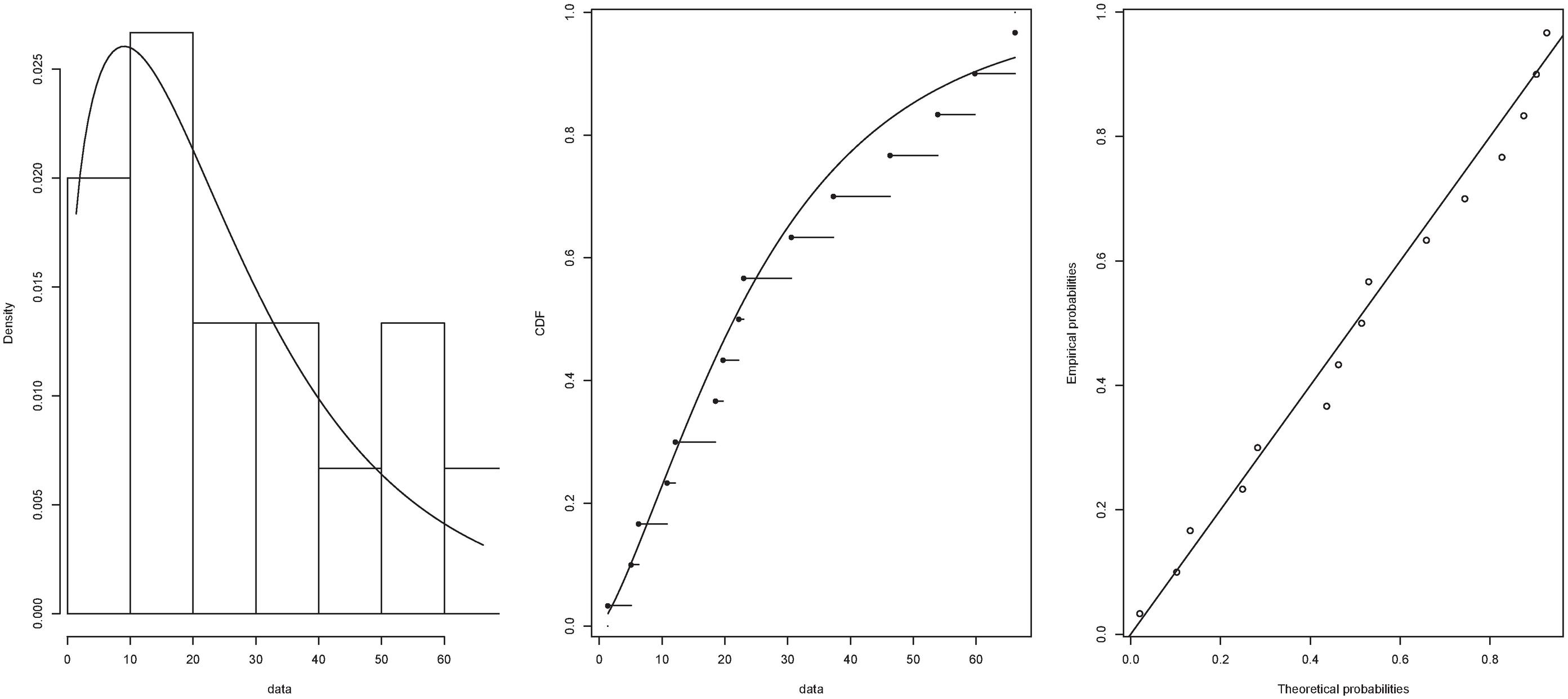
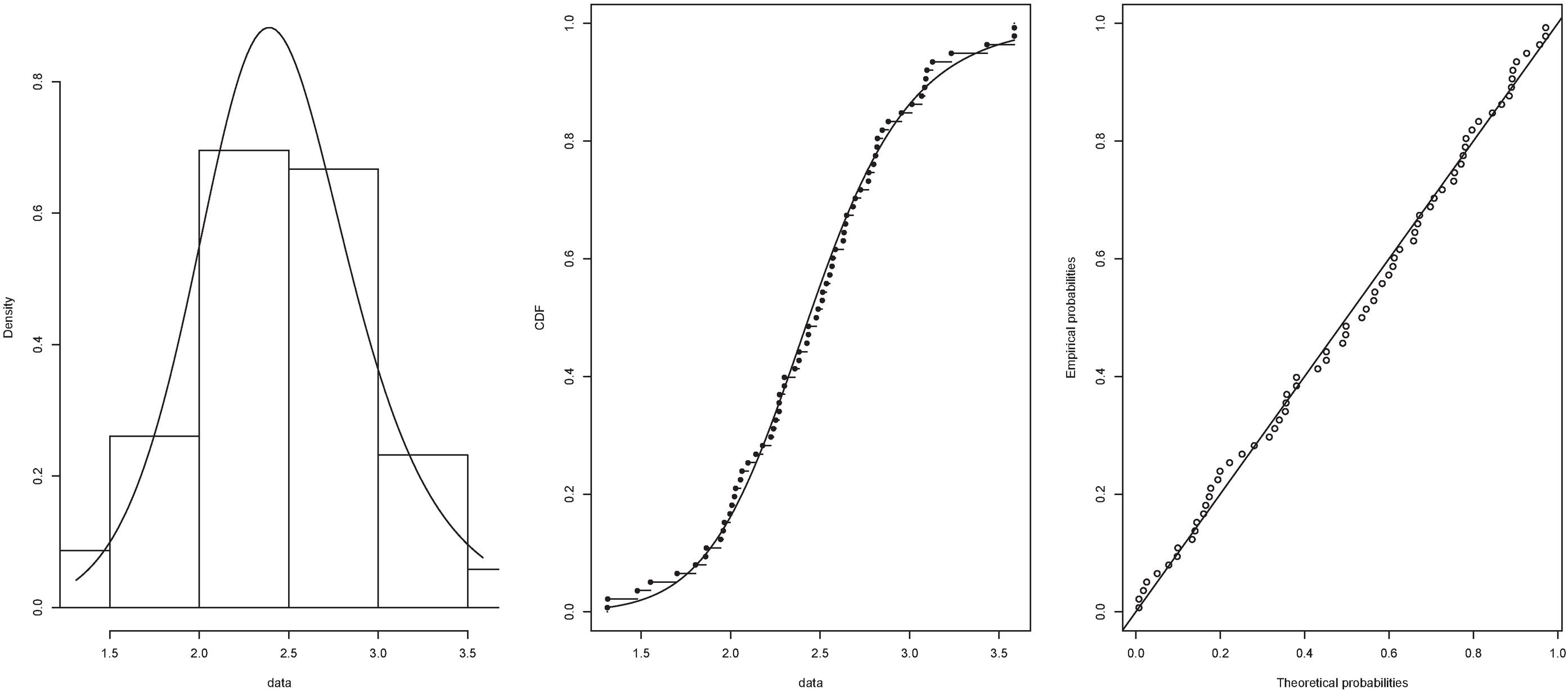
Figure 3 Histogram density, emprical and theoretical CDFs and P-P plot of data I.

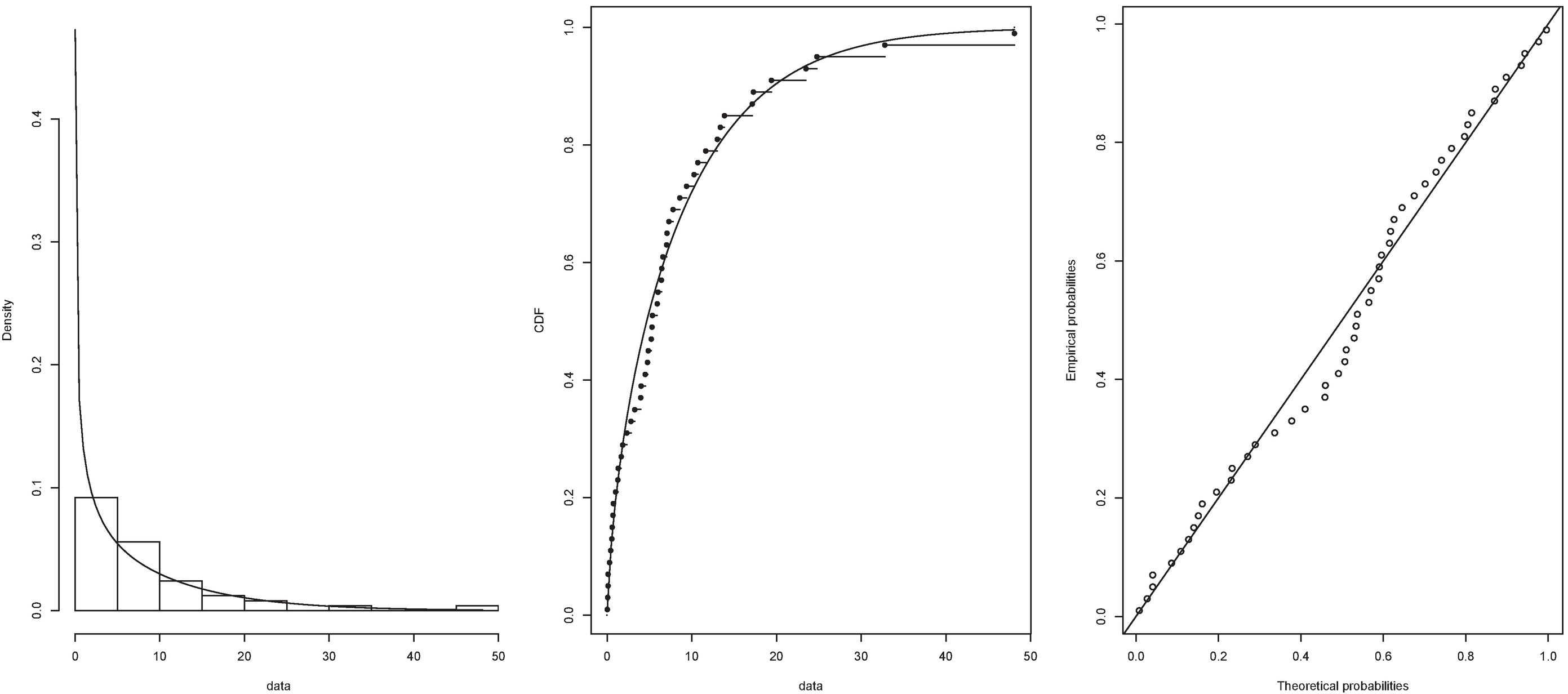
Figure 4 Histogram density, emprical and theoretical CDFs and P-P plot of data II.

Figure 5 Histogram density, emprical and theoretical CDFs and P-P plot of data III.

Figure 6 Histogram density, emprical and theoretical CDFs and P-P plot of data IV.

5 Conclusions

In this paper, reliability test plan based on LoED is introduced. To illustrate the practical applicability we have discussed four numerical example. Minimum sample sizes are provided in Tables for Binomial and Poisson approximations, respectively. The OC values for specified plan are presented in Tables for proposed plan. Also, minimum ratio of $Med/Me{d}_0$ are computed in the paper and placed in Tables to ensure the acceptability of lot with producer’s risk $0.05$. Findings of the proposed reliability test plan are also discussed. Suggested methodology can be used for the other skewed or symmetric distributions and will used in the industry. Thus, in a nutshell our paper helps the young practitioners in field of reliability analysis helping them to arrive at quick estimates they require in almost no span of time.

References

[1] Lan, Y., and Leemis, L. M. (2008). The logistic–exponential survival distribution. Naval Research Logistics (NRL), 55(3), 252–264.

[2] Sobhi, A. L., and Mashail, M. (2020). The Inverse-Power Logistic-Exponential Distribution: Properties, Estimation Methods, and Application to Insurance Data. Mathematics, 8(11), 2060.

[3] Ali, S., Dey, S., Tahir, M. H., and Mansoor, M. (2020). Two-Parameter Logistic-Exponential Distribution: Some New Properties and Estimation Methods. American Journal of Mathematical and Management Sciences, 39(3), 270-298.

[4] Elgarhy, M., ul Haq, M. A., and Perveen, I. (2019). Type-II half logistic exponential distribution with applications. Annals of Data Science, 6(2), 245–257.

[5] Goode, H. P., and KAO, J. H. (1961). Sampling plans based on the Weibull distribution. Cornell University Ithaca New York.

[6] Gupta, S. S., and Gupta, S. S. (1961). Gamma distribution in acceptance sampling based on life tests. Journal of the American Statistical Association, 56(296), 942–970.

[7] Kantam, R. R. L., Rosaiah, K., and Rao, G. S. (2001). Acceptance sampling based on life tests: log-logistic model. Journal of applied statistics, 28(1), 121–128.

[8] Rosaiah, K., and Kantam, R. R. L. (2005). Acceptance sampling based on the inverse Rayleigh distribution. De Gruyter, 20(2), 277–286.

[9] Gupta, R. C., Ghitany, M. E., and Al-Mutairi, D. K. (2010). Estimation of reliability from Marshall–Olkin extended Lomax distributions. Journal of Statistical Computation and Simulation, 80(8), 937–947.

[10] Rosaiah, K., Kantam, R. R. L., and Kumar, S. (2006). Reliability test plans for exponentiated log-logistic distribution. De Gruyter, 21(2), 279–289.

[11] Rao, G. S., Ghitany, M. E., and Kantam, R. R. L. (2009). Reliability test plans for Marshall-Olkin extended exponential distribution. Applied mathematical sciences, 3(55), 2745–2755.

[12] Krishna, E., Jose, K. K., Alice, T., and Ristić, M. M. (2013). The Marshall-Olkin Fréchet distribution. Communications in Statistics-Theory and Methods, 42(22), 4091–4107.

[13] Jose, K. K., and Sivadas, R. (2015). Negative binomial Marshall–Olkin Rayleigh distribution and its applications. Economic Quality Control, 30(2), 89–98.

[14] Jose, K. K., and Joseph, J. (2018). Reliability test plan for the gumbel-uniform distribution. Stochastics and Quality Control, 33(1), 71–81.

[15] Gillariose, J., and Tomy, L. (2021). Reliability Test Plan for an Extended Birnbaum-Saunders Distribution. Journal of Reliability and Statistical Studies, 353–372.

[16] Ravikumar, M.S., Durgamamba, A.N., and Kantam, R.R.L. (2019). Economic reliability test plan for Burr Type X distribution. International Journal of Advanced Engineering Research and Applications, 5(3), 56–63.

[17] Rosaiah, K., Rao, G.S., Kalyani, K. & Shivakumar, D.C.U. (2017). Odds Exponential Log-Logistic Distribution – An economic reliability test plan. International Journal of Science and Research, 7(11):1653–1660.

[18] Kaviayarasu, V., and Fawaz, P. (2017). A Reliability sampling plan to ensure percentiles through Weibull Poisson distribution. International Journal of Pure and Applied Mathematics, 117(13), 155–163.

[19] Lawless, J. F. 2003. Statistical models and methods for lifetime data. Wiley, New York.

[20] Tripathi, H., Dey, S., and Saha, M. (2021a). Double and group acceptance sampling plan for truncated life test based on inverse log-logistic distribution. Journal of Applied Statistics, 48(7), 1227–1242.

[21] Tripathi, H., Al-Omari, A. I., Saha, M., and Alanzi, A. R. (2021b). Improved Attribute Chain Sampling Plan for Darna Distribution. Computer Systems Science and Engineering, 38(3), 381–392.

[22] Murthy D., Xie, M. & Jiang, R., (2004): Weibull Models. Wiley series in Probability and Statistics. John Wiley and Sons, NJ, 43(1), 1–29.

[23] Jose, K., and Paul, A. (2018). Marshall Olkin exponential power distribution and its generalization: Theory and Applications. IAPQR Transactions, 43(1).

[24] Bader, M. G., and Priest, A. M. (1982). Statistical aspects of fibre and bundle strength in hybrid composites. Progress in science and engineering of composites, 1129–1136.

Biographies

Abhimanyu Singh Yadav. Currently he is working as an assistant professor in Department of Statistics, Banaras Hindu University, India. His research area is: distribution theory, Bayesian and classical estimation, relibility theory. He has published more than 40 papers in reputed national and international journals.

Mahendra Saha. Currently he is working as an assistant professor in Department of Statistics, Central University of Rajasthan, India. His research area is: distribution theory, Bayesian and classical estimation, statistical quality control. He has published more than 40 papers in reputed national and international journals.

Shivanshi Shukla. Currently she is a research scholor in Department of Statistics, Central University of Rajasthan, India. Her research area is: distribution theory, Bayesian and classical estimation. She has published 2 papers in reputed international journals.

Harsh Tripathi. Currently he is working an assistant professor in Department of Mathematics, Lovely Professional University, Punjab, India. His research area is: distribution theory, Bayesian and classical estimation and statistical quality control. He has published 6 papers in reputed national and international journals.

Rajashree Dey. She was a M.Sc student in Department of Statistics, Central University of Rajasthan, India. Her area of interest is reliability test plan.

Journal of Reliability and Statistical Studies, Vol. 14, Issue 2 (2021), 695–724.
doi: 10.13052/jrss0974-8024.14215
© 2021 River Publishers