Regional Frequency Analysis of Maximum Monthly Rainfall in Haryana State of India Using L-Moments
Mohit Nain* and B. K. Hooda
Department of Mathematics and Statistics, College of Basic Sciences and Humanities, CCS Haryana Agricultural University, Hisar-125004 (Haryana), India
E-mail: nainbir93@gmail.com
*Corresponding Author
Received 24 July 2020; Accepted 08 January 2021; Publication 15 March 2021
Abstract
The paper aims to select the appropriate regional frequency distribution for the maximum monthly rainfall and estimation of quantiles using L-moments for the 27 rain gauge stations in Haryana. These 27 rain gauge stations were grouped into three homogeneous regions (Region-1, Region-2, and Region-3) using Ward’s method of cluster analysis. To confirm the homogeneity of each region, L-moments based measure of heterogeneity was used. For each homogeneous region, a regional distribution was selected with the help of the L-moments ratio diagram and goodness-of-fit test. Results of the goodness-of-fit test and L-moments ratio diagram indicated that Generalized Logistic and Generalized Extreme Value distributions were best- fitted regional frequency distributions for the Region-1 and Region-2 respectively while for Region-3, Pearson Type-3) was best-fitted distribution. The quantiles for each region were calculated and the regional growth curves were developed. The accuracy measurements were determined using Monte Carlo simulations for the regional quantiles. Results of simulations showed that uncertainty in regional quantiles measured by Root Mean Square Error value and 90 percent error limits were small when the return period was low but uncertainty in quantiles increases as the return period increases.
Keywords: Maximum monthly rainfall, cluster analysis, L-moments, regional frequency analysis, return period, quantile estimates.
1 Introduction
The occurrence of extreme events like extreme rainfall, extreme temperature, and floods may have a long-term adverse impact on human society. Hydrologists are always interested to know the probability of occurrence of such types of extreme events. The three extreme value distributions have been used for a long for estimating probabilities of maximum and minimum values for many samples. Hooda et al. (1990, 1991) derived maximum likelihood estimates of Type-1 and Type-II extreme value distribution parameters from type-II censored samples.
Advanced information about high rainfall magnitudes and frequencies is essential for sustainable management of water bodies, the creation of hydraulic systems such as dams, and planning for water-related natural hazards. Frequency analysis is the estimate of how frequently a specified event will take place. Two different approaches for frequency analysis of extreme weather like rainfall and floods are used, one of which is at-site frequency analysis while the other is called regional frequency analysis. Due to unequal record duration and insufficient data, at-site frequency methods may be affected by sampling variability, especially when return periods exceed the duration of observed data at a site (Cunnane, 1988, Hosking and Wallis, 1993). Regional Frequency Analysis (RFA) procedure based on L-moments combines data from many sites that have similar statistical characteristics in a selected region, and a single frequency distribution is valid in that area after scaling by a site-specific scaling factor (Gabriele and Arnell, 1991). The regional method is also considered to increase the precision of the estimate because it decreases the uncertainty of sampling by pooling data from multiple sites. L-moment estimators are less sensitive to the largest observations in a sample as compared to ordinary product-moment estimators, since these are linear combinations of ordered observations, whereas ordinary product-moment estimators include square or cube observations. L-moments have a superior capacity to discriminate between different distributions as compare to traditional moments, since the L-moment estimators of location, scale, and shape are almost unbiased, regardless of the probability distribution from which the observations emerge (Hosking 1990; Hosking and Wallis 1997; Zafirakou-Koulouris et al. 1998).In the case of highly skewed data, the L-moments are especially good at identifying the distributional properties whereas ordinary product-moment diagrams are almost useless for this job (Vogel and Fennessey 1993; Hosking and Wallis 1997).
RFA approach based on the L-moments method involves the suitability of the data, detection of homogeneous regions/groups, and selection of regional frequency distribution and quantiles estimation for selected distribution. Many studies have been conducted using RFA based on the L-method in a different part of the world, some of these are; Malekinezhad and Garizi (2014), Majumder et al. (2015), Liu et al. (2015), Ahmad et al. (2017), Hussain et al. (2017), Khan et al. (2017) and Dad and Benabdesselam (2018). Past studies of rainfall distribution in Haryana include Hooda (1998, 2006), Babu and Hooda (2018), and Nain and Hooda (2019a). But none of these studies in Haryana have used the L-moments approach for the estimation of rainfall quantiles.
This paper aims to identify homogeneous regions via cluster analysis and find suitable regional frequency distributions for each homogeneous region using L-moment ratio diagrams and L-moments based goodness-off-fit test. Five frequency distributions, namely the General Extreme Value (GEV), Generalized Logistic (GLO), Generalized normal (GNO), Pearson types-3 (PE3) and Generalized Pareto (GPA), have been investigated. This study will provide useful information to establish the most acceptable distribution for rainfall data from the rainfall series data used in the planning, design, and management of water resource management projects in the region.
2 Materials and Methods
2.1 Rainfall Data
In this study, monthly maximum rainfall data from 1970 to 2017 have been used. The rainfall data were obtained from the National Data Centre, Indian Meteorological Department (IMD) Pune covering the 27 rain gauge stations scattered in all the districts of Haryana state. The name of the rain gauge stations and their geographical locations are presented in Figure 1.
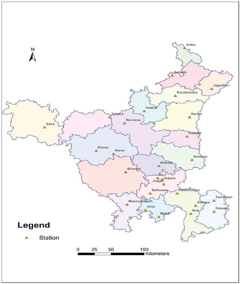
Figure 1 Rain gauge stations with geographical location.
2.2 Methods of the L-moments
The details about the method of L-moments are presented in (Hosking and Wallis, 1997) but in short, it is a modification of the probability-weighted moments (PWMs) of Greenwood et al. (1979). L-moments and L-moment ratios are more convenient than probability-weighted moments because they are more easily interpretable as measures of distribution’s scale and shape (Hosking, 1994).
Hosking (1990) introduced the L-moments which are modifications of the probability-weighted moments (PWMs) and derived as linear combinations of PWMs. Greenwood et al. (1979) defined the PWMs for a random variable X with CDF F(x) as
| (1) |
where , and are the real numbers. A very simple and useful functional case of the probability-weighted moments is .
| (2) |
In term of PWMs, the L-moments are given by:
| (3) |
Hosking (1990) also defined the L-moments ratios as:
| L-coefficient of variation (L-CV,) | |
| L-skewness (L-Cs,) | |
| L-kurtosis (L-Ck, ) |
For an ordered sample , the sample estimate of (Landwehr et al., 1979) is given as
Hence,
| (4) |
are the first four L-moments of the sample. Also, , and are the sample L-coefficient of variation, L-skewness, and L-kurtosis respectively.
2.3 Methodology of RFA
2.3.1 Clustering of rain-gauge stations or formation of homogenous regions
The formation of homogenous regions is an essential step for the RFA. Nain and Hooda (2019b) used Ward’s clustering method and found that it provides better results than other commonly used clustering methods. Hence, Ward’s (1963) clustering method was used for grouping of the rain gauge stations. Clustering was done based on the average monthly rainfall of all 27 rain gauge stations.
2.3.2 Data screening
Hosking and Wallis (1993) suggested a measure of discordancy based on L-moments to find distinct sites within a group of sites. This test determines any high discordant site which has different L-moment ratios from the group. The test for the site is calculated as:
| (5) |
where vector contains sample L-moment ratios for site i, is the total sites in the region, denotes the region’s unweighted average of L-moments ratio, and is the sample covariance matrix. A site is identified as a discordant site from the group if its value exceeds the critical value. will be the critical value for sites.
2.3.3 Heterogeneity test
Hosking and Wallis (1993) also suggested a heterogeneity test for checking the homogeneity of formed regions. For this four-parameter Kappa distribution was fitted to the regional L-moments ratios and 500 repeated Monte Carlo simulations were generated using this Kappa distribution. The generated regions in the simulations have the same number of sites, record lengths as the actual region. The heterogeneity test compares the variability of the real region’s L-moment ratios with the simulated regions. The three measures of heterogeneity ( and ) were calculated as:
| (6) |
where is the mean and is the standard deviation of simulated values. V-statistic is as follows:
| (7) | ||
| (8) | ||
| (9) |
where, and are L-moments ratios for a given region. Thus, according to Hosking and Wallis (1993), if , the region is acceptably homogeneous; if , region is acceptably heterogeneous and if , the region is acceptably heterogeneous. Also, they found that has greater power to discriminate between heterogeneous and homogeneous region as compared to and .
2.3.4 Selection of a suitable regional frequency distribution
For the selection of regional frequency distribution, two methods were used, the L-moment ratio diagram and goodness-of-fit test. The L-moment ratio diagram is a graph between theoretical L-skewness and L-kurtosis of the candidate distributions. The regional L-skewness and L-kurtosis are plotted on this graph and distribution is chosen if the regional L-skewness and L-kurtosis is in close agreement with the theoretical L-skewness and L-kurtosis of the distribution.
The goodness of fit test () statistic measures how well the regional L-kurtosis matches with the theoretical L-kurtosis of the candidate distribution. To perform this test, Hosking and Wallis (1993) suggested a Monte Carlo simulation using four parameters Kappa distribution considering parameters equal to regional L-moments ratios . The value of the statistic was calculated as:
| (10) |
where is the L-kurtosis of the candidate distribution, is average L-kurtosis calculated for a given region using observed data, represents bias value for , and is the standard deviation of the L-kurtosis () obtained from simulation. Here and are given by
For finding a good fit distribution, compute for all candidate distributions, in the homogeneous regions and select the best fit distribution for which value of at 90% confidence interval. If more than one distribution qualifies the criterion of statistic, choose the distribution for which has a minimum value.
2.3.5 Quantiles estimation
Quantile estimation is the next step after selecting the regional frequency distribution. The regional quantiles are estimated for various non-exceedance probability () levels or return periods for each homogeneous region. At station rainfall quantiles, are estimated using the index-flood method (Hosking and Wallis, 1997). In this method, it is assumed that the rainfall of different stations in a homogenous region has the same frequency distribution except for a site-specific scale factor (Darymple, 1960). This scale factor is known as the index flood. The quantile estimates at i rain gauge station with non-exceedance probability are calculated as
| (11) |
where regional quantile estimate or regional growth curve for the region and index flood value for the site (average maximum monthly rainfall).
The accuracy of regional estimated quantiles was assessed by Monte Carlo simulation. Hosking and Wallis (1997) presented an algorithm for the simulation of the L-moment regional algorithm. According to this algorithm, a large number of reference regions are generated using Monte Carlo simulations and these reference regions have the same number of stations, record lengths at each station, and L-moment regional ratios as the original region. The possible heterogeneity and inter-site dependency in the regions are also accounted for by the generated reference regions.
Table 1 L-moments and L-moments ratios of maximum monthly rainfall of 27 rain gauge stations in Haryana
| S.No. | Station | ||||
| 1 | Sirsa | 154.33 | 0.27 | 0.153 | 0.177 |
| 2 | Narwana | 200.021 | 0.290 | 0.153 | 0.084 |
| 3 | Hisar | 167.863 | 0.249 | 0.115 | 0.176 |
| 4 | Karnal | 278.356 | 0.224 | 0.097 | 0.071 |
| 5 | Ambala | 297.777 | 0.185 | 0.208 | 0.250 |
| 6 | Jhajjar | 239.739 | 0.271 | 0.130 | 0.047 |
| 7 | Hansi | 111.727 | 0.312 | 0.268 | 0.137 |
| 8 | Sonipat | 261.487 | 0.254 | 0.166 | 0.132 |
| 9 | Rohtak | 214.803 | 0.276 | 0.100 | 0.076 |
| 10 | Panipat | 210.958 | 0.262 | 0.143 | 0.099 |
| 11 | Farukhnagar | 191.856 | 0.344 | 0.197 | 0.217 |
| 12 | Faridabad | 256.224 | 0.244 | 0.205 | 0.216 |
| 13 | Kurukshetra | 225.420 | 0.297 | 0.222 | 0.116 |
| 14 | Mahendragarh | 168.708 | 0.303 | 0.236 | 0.238 |
| 15 | Kaithal | 217.858 | 0.274 | 0.141 | 0.067 |
| 16 | Khol | 141.079 | 0.356 | 0.169 | 0.161 |
| 17 | Palwal | 211.058 | 0.257 | 0.318 | 0.309 |
| 18 | Bhiwani | 145.872 | 0.270 | 0.172 | 0.096 |
| 19 | Tohana | 151.323 | 0.283 | 0.115 | 0.140 |
| 20 | Sohana | 225.158 | 0.261 | 0.149 | 0.100 |
| 21 | Bawal | 237.758 | 0.213 | 0.112 | 0.217 |
| 22 | Jagadhari | 370.504 | 0.251 | 0.289 | 0.241 |
| 23 | Dujana | 209.315 | 0.308 | 0.161 | 0.132 |
| 24 | Salhawas | 167.579 | 0.347 | 0.295 | 0.263 |
| 25 | Nuh | 257.627 | 0.264 | 0.167 | 0.215 |
| 26 | Kalka | 386.581 | 0.234 | 0.153 | 0.212 |
| 27 | Beri | 206.223 | 0.322 | 0.183 | 0.109 |
In this procedure, the number of reference regions which are generated was set to 10,000, and the number of simulations was set to 500 for each homogeneous region. The best fitted regional distribution was used in the simulation for each homogeneous region. For this simulated data RMSE values and 90 percent error limits were calculated for each homogeneous region.
Statistical analyses: Analysis and graphics were obtained using RStudio version 1.2.1335. For L-moment analysis, the R package lmomRFA developed by Hosking and Wallis (2009) was used. This package implements methods mentioned in the book “Regional frequency analysis: an approach based on L-moments” by J. R. M. Hosking and J. R. Wallis (1997). Please search https:/CRAN.R-project.org/package=lmomRFA for more information on this package.
3 Results and Discussion
The initial assumptions of stationarity, independence, and randomness of the data were checked using the Mann-Kendall test, autocorrelation plot, and Wald-Wolfowitz run test, respectively. The data were found suitable for regional frequency analysis. To carry out RFA, the maximum monthly rainfall (highest rainfall recorded month in each year) of 27 rain gauge stations in Haryana has been analyzed. The name of rain gauge stations and their L-moments ratios are presented in Table 1.
3.1 Cluster Analysis
Hierarchical cluster analysis with Ward’s method has been used to group various rain gauge stations into different regions. It divided the 27 rain gauge stations into 3 regions which are shown in Figure 2. The Region-1 contains 4 stations, Region-2 contains 13 stations and Region-3 contains 10 stations.
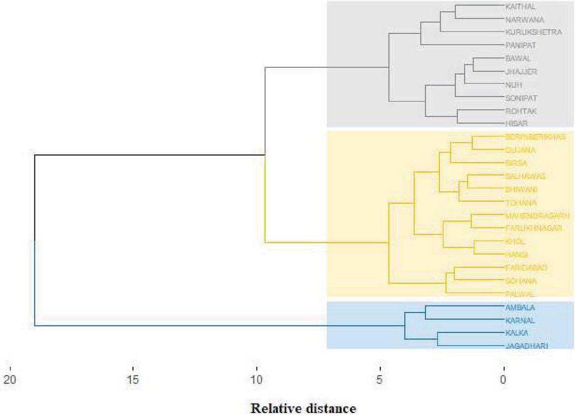
Figure 2 Cluster dendrogram.
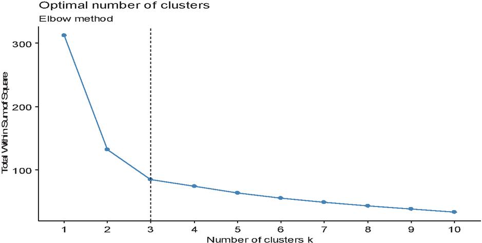
Figure 3 Elbow graphic, best .
The Elbow method and the NbClust package were used for deciding the optimal number of clusters. The Elbow approach dealt with the total Within Sum of Squares (WSS) as a function of cluster number and one should select a number such that adding another cluster will not significantly improve the total WSS. There is a sharp decrease in total WSS from cluster-1 to cluster-3, and after that, there is a small decrease in total WSS (Figure 3). Hence, the optimal number of clusters or regions suggested by the Elbow method is three.
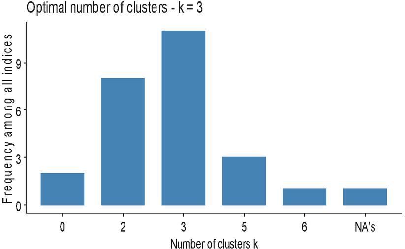
Figure 4 Optimal number of cluster provided by NbClust package.
In addition to the Elbow method, the NbClust package (Charrad et al., 2014) was also used, which provides several indices for deciding the optimal number of clusters. This package used 25 indices, and according to the majority rule, the optimal number of clusters or regions is 3 regions (Figure 4). Therefore, the optimal number of regions selected using both criteria came out to be 3.
3.2 Discordancy, Homogeneity and Goodness-of-fit ()
Discordancy measure () and regional L-moments are presented in Table 2. For regions-1, 2 & 3, all stations have values less than the corresponding critical values 1.33, 2.87, and 2.49, respectively which means that there were no discordant stations in these regions. Heterogeneity tests (H) for each region are presented in Table 3. The results revealed that all three regions can be considered as homogeneous based on Heterogeneity test criteria.
Table 2 Discordance measures and regional L-moments for three homogeneous regions
| Station Name | Regional L-moments | ||
| Region-I | Ambala | 1.00 | |
| Karnal | 1.00 | ||
| Jagadhari | 1.00 | ||
| Kalka | 1.00 | ||
| Region-2 | Sirsa | 0.64 | |
| Hansi | 1.97 | ||
| Farukhnagar | 0.97 | ||
| Faridabad | 0.96 | ||
| Mahendragarh | 0.32 | ||
| Khol | 1.12 | ||
| Palwal | 2.15 | ||
| Bhiwani | 0.89 | ||
| Tohana | 0.94 | ||
| Sohana | 0.82 | ||
| Dujana | 0.22 | ||
| Salhawas | 1.36 | ||
| Beri | 0.64 | ||
| Region-3 | Hisar | 0.72 | |
| Sonipat | 0.77 | ||
| Rohtak | 1.40 | ||
| Nuh | 1.53 | ||
| Jhajjar | 0.79 | ||
| Bawal | 1.85 | ||
| Panipat | 0.24 | ||
| Kurukshetra | 1.79 | ||
| Narwana | 0.54 | ||
| Kaithal | 0.36 |
Table 3 Heterogeneity measures for homogeneous regions
| Region-1 | 0.17 | 0.06 | 0.24 |
| Region-2 | 0.57 | 0.74 | 0.63 |
| Region-3 | 0.27 | 2.06 | 0.50 |
The values for all three regions are also presented in Table 4. For Region-1, GLO, GEV, and GNO distributions satisfied the goodness of fit criterion while GLO was observed to be the best-fitted distribution because of the lowest critical || value. For Region-2, GLO, GEV, and GNO distributions were good fitted but the best-fitted distribution was GEV due to the smallest || value. In the case of Region-3, GEV, GNO, and PE3 distributions are found to be the good fit distributions where PE3 is the best-fitted distribution because of its lowest || value among all three distributions.
Table 4 measure and parameter estimation for three homogeneous regions
| Parameters | |||||
| Distributions | Z-value | ||||
| Region-I | GLO | 0.9324 | 0.2111 | -0.1869 | - 0.10^** |
| GEV | 0.8099 | 0.3149 | -0.0262 | -1.18^* | |
| GNO | 0.9254 | 0.3727 | -0.3856 | - 1.39^* | |
| Region-II | GLO | 0.9038 | 0.2813 | -0.1985 | 1.32^* |
| GEV | 0.7414 | 0.4154 | -0.0439 | -0.72^** | |
| GNO | 0.8939 | 0.4964 | -0.4100 | -1.19^* | |
| Region-III | GEV | 0.7866 | 0.3958 | 0.0398 | 1.20^* |
| GNO | 0.9312 | 0.4523 | -0.2974 | 1.08^* | |
| PE3 | 1.0000 | 0.4808 | 0.8800 | 0.44^** | |
| (where * implies fitted distributions and ** implies best-fitted distributions). | |||||
Region-wise L-moments ratio diagrams are given in Figure 5. These diagrams indicate that GLO distribution is the best fitted for Region-1 (Figure 5(a)), GEV distribution for Region-2 (Figure 5(b)), and PE3 distribution is the best fitted for Region-3 (Figure 5(c)). It was observed that results obtained using the L-moments ratio diagram confirm the results obtained from test.
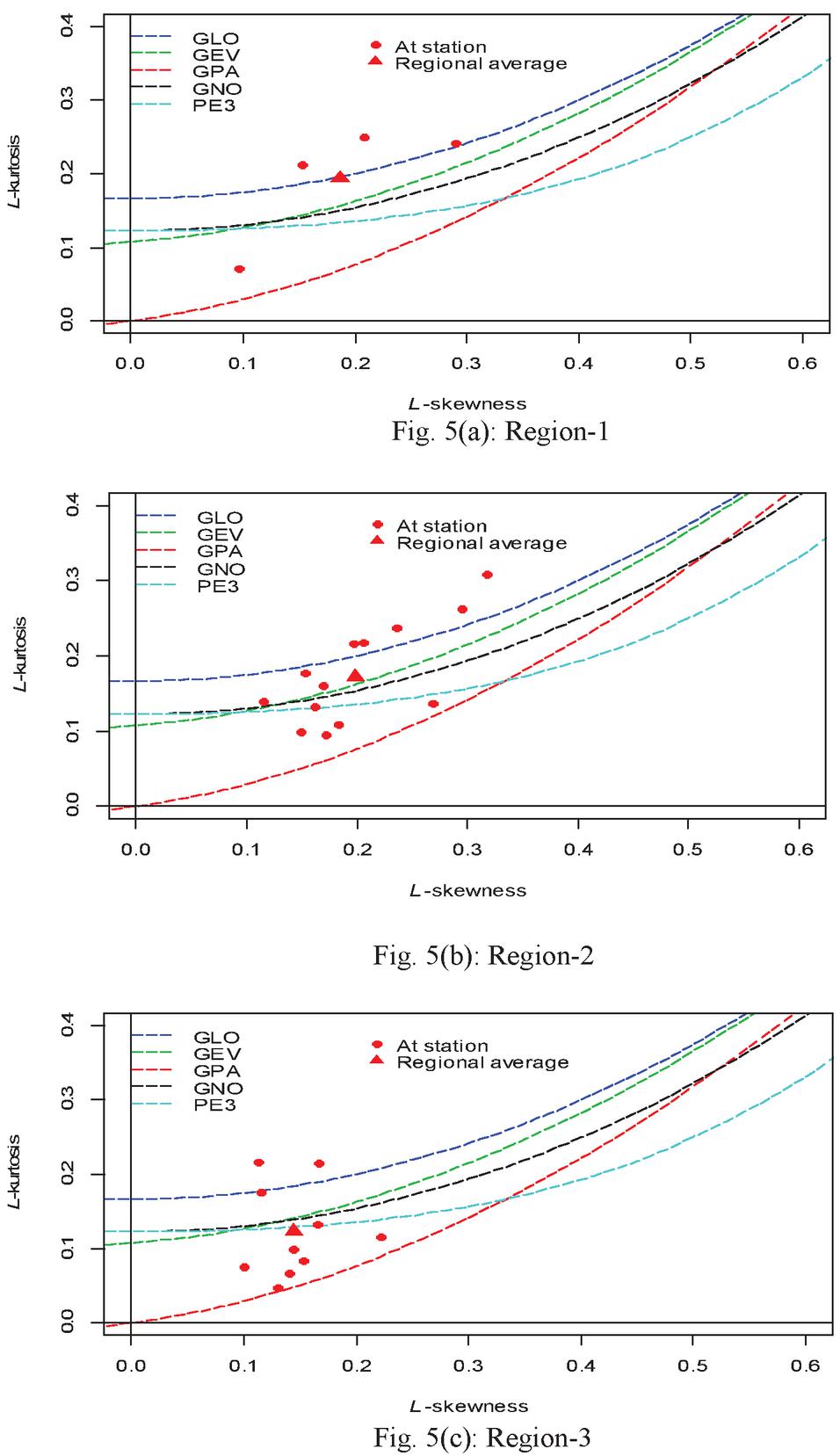
Figure 5 L-moments ratio diagrams for all three regions.
3.3 Estimation of Quantiles and Regional Growth Curve
Regional quantiles for three homogeneous regions are given in Table 5. The values of the quantiles can be explained as, for example, for Region-2, is the amount of rainfall that will happen once in 100 years and is 2.785 times larger than its average rainfall for all rain gauge stations in the homogeneous Region-2. Thus, all estimated quantiles for all the three regions can be explained in this way.
Table 5 Regional quantile estimates, for three regions for the fitted distributions
| Region-1 | Region-2 | Region-3 | ||||||||
| Fitted Distributions | Fitted Distributions | Fitted Distributions | ||||||||
| F | T | GLO | GEV | GNO | GLO | GEV | GNO | GEV | GNO | PE3 |
| 0.5 | 2 | 0.932 | 0.926 | 0.925 | 0.904 | 0.895 | 0.894 | 0.931 | 0.931 | 0.930 |
| 0.8 | 5 | 1.266 | 1.292 | 1.296 | 1.353 | 1.386 | 1.393 | 1.363 | 1.364 | 1.371 |
| 0.9 | 10 | 1.506 | 1.540 | 1.543 | 1.679 | 1.724 | 1.731 | 1.639 | 1.637 | 1.644 |
| 0.95 | 20 | 1.761 | 1.782 | 1.781 | 2.029 | 2.059 | 2.059 | 1.895 | 1.891 | 1.892 |
| 0.98 | 50 | 2.140 | 2.104 | 2.093 | 2.555 | 2.510 | 2.493 | 2.217 | 2.212 | 2.197 |
| 0.99 | 100 | 2.469 | 2.349 | 2.329 | 3.014 | 2.859 | 2.825 | 2.450 | 2.448 | 2.416 |
| 0.995 | 200 | 2.840 | 2.599 | 2.569 | 3.539 | 3.218 | 3.164 | 2.676 | 2.682 | 2.627 |
| 0.998 | 500 | 3.410 | 2.935 | 2.891 | 4.350 | 3.709 | 3.623 | 2.965 | 2.990 | 2.897 |
| (T denote the return periods, and F denote the non-exceedance probability). | ||||||||||
Regional growth curves (with 90% error limits) were constructed for each region for the best fitted regional frequency distribution and are presented in Figure 6(a)–6(c) respectively. The growth curve specifies the quantiles corresponding to different return periods. From the regional growth curve, it was found that error bounds were wider for large return periods as compare to small return periods, so it indicates that unreliability of regional quantiles increases with an increase in return periods for all the regions (Figure 6).
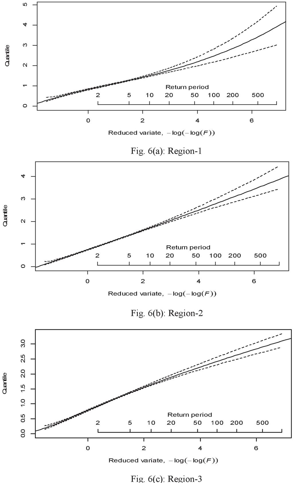
Figure 6 Regional growth curves for all three regions.
At station quantile estimates for 100 years return period have been obtained by multiplying the regional quantiles of best-fitted distribution with the stations’ average rainfall (). Table 6 shows the estimated quantiles for 27 rain gauge stations up to 100 years return period. Accuracy measures like RMSE value and 90% error bounds of regional quantiles were also obtained by using Monte Carlo simulation for each region and are presented in Table 7. Results showed that the RMSE values increase if the return period goes on increasing, which suggested the unreliability of quantiles for the high return period.
Table 6 Estimated maximum monthly rainfall (mm) quantiles corresponding to different return periods using best fitted regional frequency distribution
| Non-exceedance Probability | ||||||||
| 0.5 | 0.8 | 0.9 | 0.95 | 0.98 | 0.99 | |||
| No. | Station | 2 | 5 | 10 | 20 | 50 | 100 | |
| 1 | Ambala | 277.5 | 377.0 | 448.5 | 524.4 | 637.2 | 735.2 | |
| 2 | Karnal | 259.4 | 352.4 | 419.2 | 490.2 | 595.7 | 687.3 | |
| 3 | Jagadhari | 345.3 | 469.1 | 558.0 | 652.5 | 792.9 | 914.8 | |
| 4 | Kalka | 360.3 | 489.4 | 582.2 | 680.8 | 827.3 | 954.5 | |
| 5 | Sirsa | 139.2 | 214.6 | 265.4 | 314.9 | 379.8 | 429.3 | |
| 6 | Hansi | 100.9 | 155.5 | 192.4 | 228.3 | 275.3 | 311.2 | |
| 7 | Farukhnagar | 173.3 | 267.1 | 330.4 | 392.0 | 472.7 | 534.3 | |
| 8 | Faridabad | 231.4 | 356.7 | 441.2 | 523.5 | 631.3 | 713.6 | |
| 9 | Mahendragarh | 152.3 | 234.8 | 290.5 | 344.7 | 415.7 | 469.9 | |
| 10 | Khol | 127.4 | 196.4 | 242.9 | 288.2 | 347.6 | 392.9 | |
| 11 | Palwal | 190.6 | 293.8 | 363.4 | 431.2 | 520.0 | 587.8 | |
| 12 | Bhiwani | 119.0 | 183.5 | 227.0 | 269.3 | 324.8 | 367.1 | |
| 13 | Tohana | 132.2 | 203.9 | 252.2 | 299.2 | 360.9 | 407.9 | |
| 14 | Sohana | 192.3 | 296.4 | 366.6 | 435.0 | 524.6 | 593.0 | |
| 15 | Dujana | 189.0 | 291.4 | 360.4 | 427.6 | 515.8 | 582.9 | |
| 16 | Salhawas | 151.3 | 233.3 | 288.6 | 342.4 | 412.9 | 466.7 | |
| 17 | Beri | 186.2 | 287.1 | 355.1 | 421.3 | 508.1 | 574.3 | |
| 18 | Hisar | 156.1 | 230.1 | 276.0 | 317.6 | 368.8 | 405.6 | |
| 19 | Sonipat | 243.2 | 358.5 | 429.9 | 494.7 | 574.5 | 631.8 | |
| 20 | Rohtak | 199.8 | 294.5 | 353.1 | 406.4 | 471.9 | 519.0 | |
| 21 | Nuh | 239.6 | 353.2 | 423.5 | 487.4 | 566.0 | 622.4 | |
| 22 | Jhajjar | 223.0 | 328.7 | 394.1 | 453.6 | 526.7 | 579.2 | |
| 23 | Bawal | 221.1 | 326.0 | 390.9 | 449.8 | 522.4 | 574.4 | |
| 24 | Paniapt | 196.2 | 289.2 | 346.8 | 399.1 | 463.5 | 509.7 | |
| 25 | Kurukshetra | 209.6 | 309.1 | 370.6 | 426.5 | 495.3 | 544.6 | |
| 26 | Narwana | 186.0 | 274.2 | 328.8 | 378.4 | 439.5 | 483.3 | |
| 27 | Kaithal | 202.6 | 298.7 | 358.2 | 412.2 | 478.6 | 526.3 | |
Table 7 Regional quantiles for the best-fitted distributions and their accuracy measures
| Return Period | 2 | 5 | 10 | 20 | 50 | 100 | 200 | 500 |
| F | 0.5 | 0.8 | 0.9 | 0.95 | 0.98 | 0.99 | 0.995 | 0.998 |
| Region-1 (GLO) | ||||||||
| 0.932 | 1.267 | 1.506 | 1.761 | 2.141 | 2.469 | 2.840 | 3.410 | |
| RMSE | 0.018 | 0.015 | 0.032 | 0.061 | 0.119 | 0.181 | 0.263 | 0.408 |
| LEB* (0.05) | 0.903 | 1.240 | 1.451 | 1.651 | 1.924 | 2.155 | 2.408 | 2.770 |
| UEB* (0.95) | 0.964 | 1.293 | 1.565 | 1.868 | 2.326 | 2.753 | 3.276 | 4.104 |
| Region-2 (GEV) | ||||||||
| 0.895 | 1.386 | 1.724 | 2.059 | 2.51 | 2.859 | 3.218 | 3.709 | |
| RMSE | 0.010 | 0.012 | 0.022 | 0.039 | 0.073 | 0.106 | 0.146 | 0.209 |
| LEB* (0.05) | 0.883 | 1.372 | 1.685 | 1.982 | 2.361 | 2.630 | 2.886 | 3.237 |
| UEB* (0.95) | 0.919 | 1.411 | 1.760 | 2.120 | 2.622 | 3.016 | 3.428 | 4.002 |
| Region-3 (PE3) | ||||||||
| 0.93 | 1.371 | 1.644 | 1.892 | 2.197 | 2.416 | 2.627 | 2.897 | |
| RMSE | 0.012 | 0.009 | 0.023 | 0.039 | 0.063 | 0.082 | 0.101 | 0.127 |
| LEB* (0.05) | 0.911 | 1.352 | 1.605 | 1.823 | 2.092 | 2.282 | 2.461 | 2.688 |
| UEB* (0.95) | 0.952 | 1.383 | 1.682 | 1.961 | 2.310 | 2.564 | 2.811 | 3.131 |
| LEB* Lower error bound, UEB* Upper error bound. | ||||||||
4 Conclusion
Regional Frequency Analysis is of great importance for planning and designing hydraulic structures by policymakers and structural engineers. The present study used L-moments for regional frequency analysis of maximum monthly rainfall of 27 rain gauge stations in Haryana. Based on the mean monthly rainfall, 27 rain gauge stations were grouped into three homogeneous regions (Region-1, Region-2, and Region-3) using Ward’s clustering method. Region-1, Region-2, and Region-3 contained 4, 13, and 10 rain gauge stations respectively.
Discordancy measures did not show any of the stations as discordant from their respective regions. Based on the L-moments ratio diagram and Z-statistic, GLO distribution was found most appropriate for Region-1, GEV distribution for Region-2, and PE3 for Region-3. The regional growth curves were also developed for three homogeneous regions with 90% error bounds. Rainfall quantiles were also computed for the individual stations for 100 years return period. The accuracy measures like RMSE value and 90 % error bounds of estimated regional quantiles were found to be relatively low for the return periods up to 100 years. It was observed that cluster analysis together with RFA based on L-moments methods can be successfully applied to estimate rainfall quantiles of maximum monthly rainfall in Haryana.
References
Ahmad, I., Abbas, A., Fawad, M., and Saghir, A. (2017). Regional Frequency Analysis of Annual Total Rainfall in Pakistan Using L-moments, NUST Journal of Engineering Sciences, 10(1), pp. 19–29.
Babu, V.B., and Hooda B. K. (2018). Fuzzy Majority Approach for Modeling Spatial and Temporal Distributions of Daily Rainfall in Western Zone of Haryana, Int. J. Agricult. Stat. Sci., 14(1), pp. 57–67.
Charrad M., Ghazzali N., Boiteau V., and Niknafs A. (2014), NbClust: An R Package for Determining the Relevant Number of Clusters In A Data Set, Journal of Statistical Software, 61(6), pp. 1–36.
Cunnane, C. (1988). Methods and Merits of Regional Flood Frequency Analysis, Journal of Hydrology, 100(1–3), pp. 269–290.
Dalrymple T. (1960). Flood Frequency Methods, U.S. Geological Survey, Water supply paper, 1543A, pp. 11–51.
Dad, S., and Benabdesselam, T. (2018). Regional frequency analysis of extreme precipitation in northeastern Algeria, Journal of water and land development, 39(1), pp. 27–37.
Gabriele, S., and Arnell, N. (1991). A Hierarchical Approach to Regional Flood Frequency Analysis, Water Resources Research, 27(6), pp. 1281–1289.
Greenwood, J. A., Landwehr, J. M., Matalas, N. C., and Wallis, J. R. (1979). Probability Weighted Moments: Definition and Relation to Parameters of Several Distributions Expressible In Inverse Form. Water Resources Research, 15(5), pp. 1049–1054.
Khan, S. A., Hussain, I., Hussain, T., Faisal, M., Muhammad, Y. S., Mohamd Shoukry, A. (2017), Regional frequency analysis of extremes precipitation using L-moments and partial L-moments, Advances in Meteorology (1), pp. 1–20.
Hooda, B. K. (1998). Seasonal Non-Seasonal ARIMA Models for Monthly Rainfall Data, Proceedings of First Annual Conference of Society of Statistics, Computer and Applications, Oct. 23–25, pp. 87–95.
Hooda, B. K. (2006). Probability Analysis of Monthly Rainfall for Agriculture Planning at Hisar, Indian Jour Soil Cons., 34(1), pp. 12–14.
Hooda, B. K., Singh, N. P., and Singh, U (1990). Estimates of the Parameters of Type-II Extreme Value Distribution from Censored Samples, Communications in statistics-Theory and methods, 19(8), pp. 3093–3110.
Hooda, B. K., Singh, N. P., and Singh, U (1991). Estimation of Gumbel Distribution Parameters of M-th Maxima from Doubly Censored Sample, STATISTICA, 51(3), pp. 339–352.
Hosking, J. R. M. (1994). The four-parameter kappa distribution. IBM Journal of Research and Development, 38, pp. 251–258.
Hosking J. R. M. and Wallis, J. R., (1997), Regional Frequency Analysis: An Approach Based on L-Moments, Cambridge University Press, U.K.
Hosking, J. R. M. (1990). L-Moments: Analysis and Estimation of Distributions Using Linear Combinations of Order Statistics, Journal of the Royal Statistical Society, Series B, 52(1), pp. 105–124.
Hosking, J. R. M., and Wallis, J. R. (1993). Some Statistics Useful in Regional Frequency Analysis, Water Resources Research, 29(2), pp. 271–281.
Hosking J. R. M., (2009). Regional Frequency Analysis using L-Moments, lmomRFA R package, Available at http://CRAN.R-project.org/package=lmomRFA.
Hussain, Z., Shahzad, M. N., and Abbas, K. (2017), Application of Regional Rainfall Frequency Analysis on Seven Sites of Sindh, Pakistan, KSCE Journal of Civil Engineering, 21(5), 1812–1819.
Landwehr, J. M., Matalas, N. C, and Wallis, J. R. (1979). Probability-weighted moments compared with some traditional techniques in estimating Gumbel parameters and quantiles. Water Resources Research, 15, pp. 1055–1064.
Liu, J., Doan, C. D., Shie-Yui Liong, Sanders, R., Dao, A. T., and Fewtrell, T. (2015). Regional Frequency Analysis of Extreme Rainfall Events in Jakarta, Natural Hazards, 75(2), pp. 1075–1104.
Malekinezhad, H., and Garizi, A. Z. (2014). Regional Frequency Analysis of Daily Rainfall Extremes using L-moments Approach, Atmosfera, 27(4), pp. 411–427.
Majumder A., Patil S.G., Noman M.D., and Biswas S. (2015), Application of L-Moments for Regional Frequency Analysis of Maximum Monthly Rainfall in West Bengal. India, Mausam, 66(2), pp. 273–280.
Nain, M., and Hooda B.K. (2019a). Probability and Trend Analysis of Monthly Rainfall in Haryana, Int. J. Agricult. Stat. Sci, 15(1), pp. 221–229.
Nain, M., Hooda, B.K. (2019b). Identification of Homogeneous Rainfall Stations in Haryana, Journal of Experimental Biology and Agricultural Sciences, 7(5), pp. 452–462.
Vogel, R. M. and Fennessey, N. M. (1993). L-moment diagrams should replace product-moment diagrams, Water Resources Research, 29, pp. 1745–1752.
Ward Jr. J.H. (1963). Hierarchical Grouping to Optimize an Objective Function, Journal of the American statistical association, 58(301), pp. 236–244.
Biographies

Mohit Nain is currently pursuing PhD under guidance of Dr. B. K. Hooda in the Department of Mathematics and Statistics, COBS&H, CCS Haryana Agricultural University, Hisar. He completed his master programme in 2016 and topic of research was “Spatial and Temporal Distribution of Monthly Rainfall in Haryana” He published more than 8 research papers in different reputed journal. He also attended more than 5 national and international conferences and participated many workshop related to statistical data analysis.

B. K. Hooda is currently working as a Professor of Statistics in the Department of Mathematics and Statistics, COBS&H, CCS Haryana Agricultural University, Hisar and has also served as its Head from 2011–2015. Earlier, he has taught at Dr. Y. S. Parmar University of Horticulture and Forestry, Nauni (Solan) in Himachal Pradesh, and at Guru Jambheshwar University of Science & Technology, Hisar. A member of various national and international associations and scientific societies, Professor Hooda has more than 60 research papers to his credit. He has been a Commonwealth fellow to the University of Leeds in 2007–08. He has guided several M.Sc. and Ph.D. students of statistics and has been in the advisory committee of hundreds of students and research scholars of Statistics and other disciplines. He has 30 years of teaching experience both at UG and PG level and has authored several teaching manuals. He often visits various universities and leading institutions of India to deliver talks on specialized topics. His areas of interest are statistical inference, multivariate analysis and machine learning and their applications for analyzing and interpreting agricultural data.
Journal of Reliability and Statistical Studies, Vol. 14, Issue 1 (2021), 33–56.
doi: 10.13052/jrss0974-8024.1413
© 2021 River Publishers