Profit Analysis of a Standby Repairable System with Priority to Preventive Maintenance and Rest of Server Between Repairs

Chhama Aggarwal, Nitika Ahlawat and S. C. Malik^*

Department of Statistics, M.D. University, Rohtak-124001, India

E-mail: aggarwalshama11@gmail.com; ahlawatnitika386@gmail.com; sc_malik@rediffmail.com

${}^{*}$Corresponding Author

Received 25 September 2020; Accepted 11 January 2021; Publication 15 March 2021

Abstract

The paper aims to bring out the profit analysis of a system with cold standby redundancy of two identical units. In the system, we keep one unit in working and the other is to back up the operation. The system requires preventive maintenance after a specific time. The server has the dual role to carry out repair activities in terms of preventive maintenance and repair of the failed unit. In addition to that, the server is allowed to take rest after each repair. There is no need of rest of the server after preventive maintenance. The provision of priority has been made for the preventive maintenance over repairs. The repairs are done to increase the efficiency and productivity level of the system. The failure rate follows exponential distribution while repair time, rest time of the server and preventive maintenance rate follow arbitrary distributions. The significant reliability characteristics including MTSF, long run availability, server busy time due to repair & preventive maintenance, expected number of repairs, expected number of preventive maintenances per unit time and profit function are obtained using the usual stochastic processes approach. For particular values of the parameters, the revenue per unit up-time and cost functions related to repair activities are considered to carry out the profit analysis of the system model. The results are shown graphically and numerically to highlight the effect of different parameters on some significant reliability characteristics

Keywords: Cold standby redundancy, stochastic process, rest of the server, preventive maintenance, priority, reliability characteristics and profit analysis.

1 Introduction

In the fast-growing technological age, it has become reasonable to put a spare unit(s) during operation of repairable systems in order to cover the risk or any emergency requirement. Over the years, cold standby redundancy has been probably one of the finest ways to make the use of such systems more effective. As a result, researchers have focused more on stochastic analysis of standby systems. It is well-known that most units operating in a useful life period, and complex systems that consist of many kinds of components, fail normally due to random causes independently over the time interval. A stochastic process is a set of outcomes of a random experiment indexed by time, and is one of the key tools needed to analyse the future behaviour quantitatively. The models have been developed by considering different failure assumptions and repair mechanisms. Goel and Shrivastava [1], Gupta et al. [2], Wu and Wu [4] and Wang et al. [5] have thoroughly discussed the reliability models of cold standby systems. Goel and Kumar [8] analysed a quick approximation method for profit analysis of a cold standby system. Over the years, researchers have suggested several repair and configuration policies for improving the system reliability. Kumar and Gupta [3] discussed the reliability analyses of a single unit M/G/1 system model with helping unit. Kumar and Singh [6] studied the reliability and sensitivity measures of a repairable system incorporating deliberate failure and reboot delay. Lado et al. [7] developed a model of a complex repairable system having two subsystems A and B which is connected in a series configuration. The system is studied using a supplementary variable technique and varies measures of system performance such as availability, reliability, (mean time to failure) MTTF and sensitivity & cost analysis have been made for particular values of the failure and repair rates. Shinde et al. [11] estimated repair rate under performance-based logistics (PBL) technique. Lado and Singh [12] and Raghav et al. [15] focused on the cost assessment of a system consisting two subsystem series configurations. In their research work, explicit expressions for reliability, availability, mean time to failure (MTTF) and cost analysis functions have been obtained. Poonia and Singh [14] presented the study of reliability measures of a complex system consisting of two subsystems, subsystem-1, and subsystem-2, in a series configuration with switching device. The repair operations are carried out continuously by the servers in most of these studies without taking any relaxation in between the repairs. It is a real fact that if server does repairs of the failed system continuously without having any break then it could have a bad impact on his health and as a result of which the efficiency of his work may be reduced.

Aggarwal and Malik [13] analysed a standby repairable system with rest of server between repairs. The idea of the rest of the server in between repairs has been proposed in that study so that the repair person can do his task more effectively. In the present study, one additional repair activity (called preventive maintenance) has been introduced in order to enhance the performance and thus efficiency of the system. By performing a regular preventive maintenance, we are assured that our system remains to operate under safe conditions and possible issues can be removed before they have a chance to cause harm to the system. A regular preventive maintenance may cause small hindrance for operation, but that is nothing compared to actual downtime caused by a breakdown. Preventive maintenance procedures take less time than emergency repairs and replacements. There is no doubt that preventive maintenance of the system after a particular running period of operation helps in minimizing the occurrence of faults. However, on the other hand, the accuracy of the system can be further enhanced by giving priority in the field of repair. In view of these observations in mind, several studies have been carried out by the researchers on stochastic study of repairable devices with the concepts of preventive maintenance and priority in repair disciplines. Barak et al. [9] obtained reliability characteristics of a redundant system by prioritizing inspection over repair. Kumar et al. [10] also introduced the concept of preventive maintenance of the system model while experimenting on a system of non-identical units.

A cold standby repair system with two similar units was therefore stochastically explored in detail by taking into account the principle of the rest of the server after each repair. After a specific duration of service, preventive maintenance of the system is carried out. However, server does not need any rest after preventive maintenance. The unit either remains in operation or in the failed state. The parameters of server’s repair and rest time obey arbitrary distributions while the unit’s failure rate is assumed constant. Stochastic process techniques (SMP & RPT) are used to extract mean time to system failure (MTSF) expressions, availability, server busy period due to repair, server busy period due to preventive maintenance, expected number of repairs, expected number of unit’s preventive maintenances and finally the profit of the system. For particular values of the parameters, the revenue per unit up-time and cost functions related to repair activities are calculated to carry out the profit analysis of the system model, the results of some significant reliability measures are obtained. The statistics are presented to demonstrate the effect of the failure rate, server rest completion rate, unit repair rate and unit preventive maintenance rate on MTSF, system model availability and profit of the system, as shown in Figures 2–4, respectively. In Figure 1, the state transition diagram of the system model is shown.

2 Notations

SMP	Semi-Markov Process.
RPT	Regenerative Point Technique.
O/Cs	The unit is in operative/cold standby mode.
$\lambda$	The unit’s constant failure rate.
$\alpha$	The unit’s preventive maintenance rate.
g(t)/G(t)	Probability density function (pdf)/Cumulative distribution function (cdf) of repair rate of the units.
r(t)/R(t)	Probability density function (pdf)/Cumulative distribution function (cdf) of rest completion rate of the Server.
f(t)/F(t)	Probability density function (pdf)/Cumulative distribution function (cdf) of preventive maintenance rate of the unit.
FUr/FWr	The failed unit undergoes for repair/failed unit is waiting for repair.
Pm/WPm	The unit undergoes for preventive maintenance/waiting for preventive maintenance.
FUR/FWR	The failed unit undergoes for repair/waiting for repair nonstop from previous state.
PM/WPM	The unit undergoes for preventive maintenance/waiting for preventive maintenance nonstop from previous state.
SUr/SUR	The technician is taking rest/taking rest nonstop from the previous state
$\oplus$	Character for Laplace Convolution
$\otimes$	Character for Laplace Steiltjes Convolution
$m_{ij}$	Contribution to mean sojourn time (${\mu }_i$) in state $S_i$ when system transits directly to state $S_j$.

3 System Description

Here, a system of a complex structure having two units in which one is in the operative mode, and other is in cold standby is analysed. All the activities like failure, repair, preventive maintenance and rest completion of the server are random in nature with respect to time. So, this system is analysed stochastically. One server is only being considered for repair activities, which attends the system instantly whenever needed. Preventive maintenance has been performed after a fixed duration of operation. And, the server does not need to take rest after preventive maintenance. There is a principle of priority to preventive maintenance over repair.

The states of the system are described as:

$S_0$: The original state in which operation of one unit is going on and the another is in cold standby mode

$S_1$: The one unit is failed and is under repair while the other unit is working

$S_2$: The one unit stops working and continuously being repaired from the earlier state, and the second unit is still fails and is awaiting repair

$S_3$: The one unit is working, another unit fails and waiting for repair continuously from previous state and the server is under rest

$S_4$: The one unit is operative; other is in the process of preventive maintenance

$S_5$: The one unit is failed and is waiting for repair and other unit is in the process of preventive maintenance.

$S_6$: The one unit is under continuous preventive maintenance from the previous state, and the other is awaiting preventive maintenance

$S_7$: The one unit fails and is waiting for repair, and the other is in the process of preventive maintenance from the earlier state.

$S_8$: The one unit is failed and waiting for repair and the other is also failed and continuously waiting for repair from the previous state, and the server is in repose

$S_9$: The one unit fails and undergoes for repair, and the other is continuously waiting for repair from the previous state.

$S_{10}$: The one unit fails and is continuously expecting repair from the previous state, other is waiting for preventive maintenance and the server is in repose continuously from the earlier state.

$S_{11}$: The one unitis in the process of preventive maintenance and the other is continually waiting for repair from the previous state.

$S_0$, $S_1$, $S_4$, and $S_5$, are regenerating states while all remaining states are non-regenerative states.

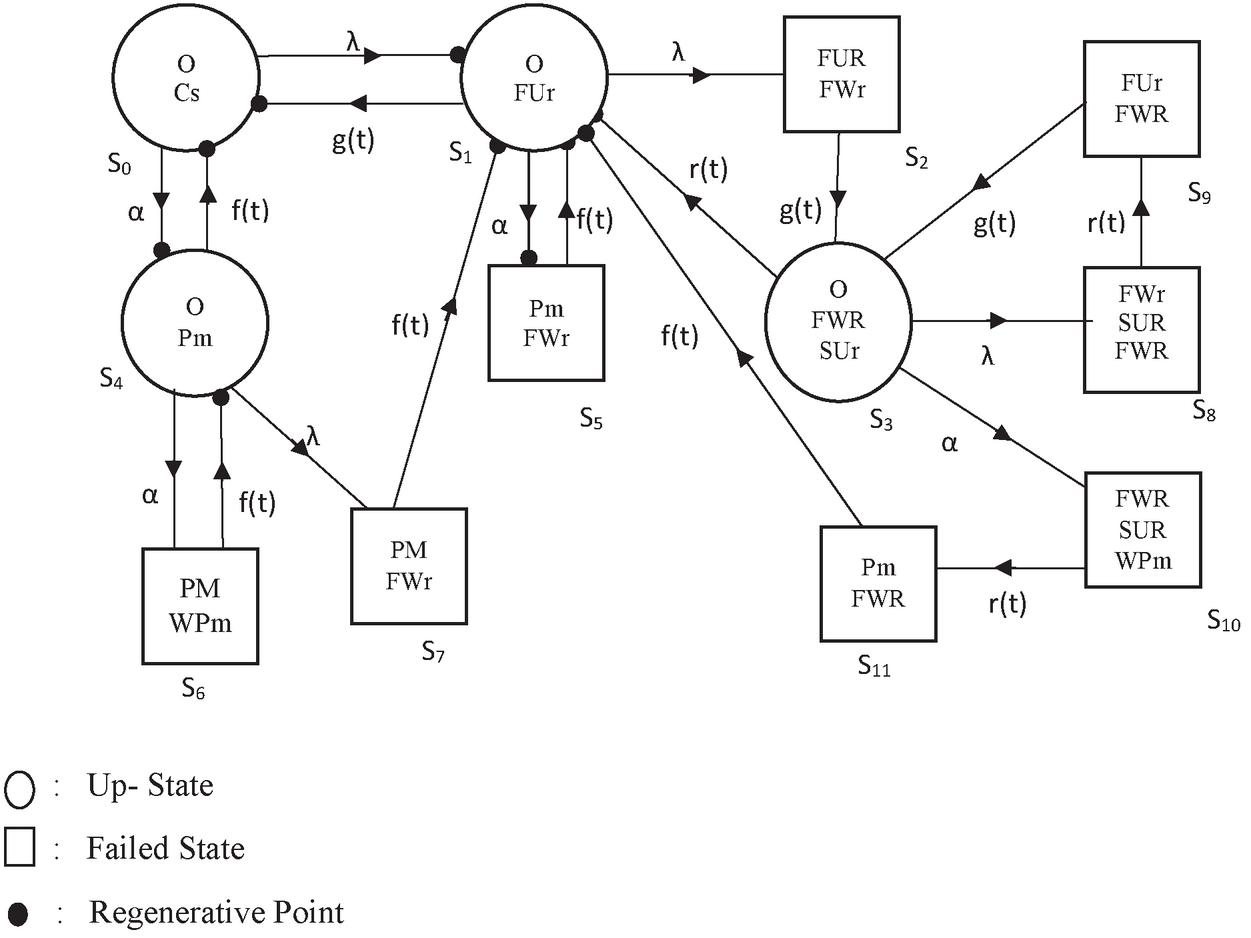
Figure 1 State transition diagram.

4 Transition Probabilities

The transition probabilities can be determined as

$$p_{ij}=Q_{ij}(\mathrm{\infty })={\int }_0^{\mathrm{\infty }}{q}_{ij}(t)\mathit{d}t$$

(1)

where, $q_{ij}(t)$ is the transition probability from state $S_i$ to $S_j$. let us consider $i=0$, then we can have $j=1$ or $j=4$. The transition probability from state $S_0$ to state $S_1$ consists of two possibilities either there is a transition from state 0 to 1 or there is no transition from state 0 to 4 i.e. System remains at state $S_0$.

Probability from state $S_0$ to $S_1$ is given by $\lambda e^{-\lambda t}$ and probability of no transition from state $S_0$ to state $S_4$ is given by $e^{-\lambda t}$. Thus we have

$$p_{01}={\int }_0^{\mathrm{\infty }}\lambda e^{-(\lambda +\alpha )t}\mathit{d}t\mathit{d}t=\frac{\lambda }{\lambda +\alpha }$$

The remaining transition probabilities are derived in similar way as follow as:

$p_{12}={\displaystyle \frac{\lambda }{\lambda +\alpha }}(1-g^{*}(\alpha +\lambda ))$	$p_{04}={\displaystyle \frac{\alpha }{\lambda +\alpha }}$
$p_{10}=g^{*}(\alpha +\lambda )$	$p_{31}=r^{*}(\alpha +\lambda )$
$p_{15}={\displaystyle \frac{\alpha }{\lambda +\alpha }}(1-g^{*}(\alpha +\lambda ))$	$p_{23}=1$
$p_{40}=f^{*}(\alpha +\lambda )$	$p_{38}={\displaystyle \frac{\lambda }{\lambda +\alpha }}(1-r^{*}(\alpha +\lambda ))$
$p_{3,10}=\frac{\alpha }{\lambda +\alpha }(1-r^{*}(\alpha +\lambda ))$	$p_{51}=1$
$p_{46}={\displaystyle \frac{\alpha }{\lambda +\alpha }}(1-f^{*}(\alpha +\lambda ))$	$p_{47}={\displaystyle \frac{\lambda }{\lambda +\alpha }}(1-f^{*}(\alpha +\lambda ))$
$p_{89}=1$	$p_{64}=1$	$p_{71}=1$
$p_{11,1}=1$	$p_{93}=1$	$p_{10,11}=1$

It can be verified that $p_{01}+p_{04}=p_{10}+p_{12}+p_{15}=p_{23}=p_{31}+p_{38}+p_{3,10}=p_{40}+p_{46}+p_{47}=p_{51}=p_{64}=p_{71}=p_{89}+p_{93}+p_{10,11}=p_{11,1}=1$.

5 Mean Sojourn Time

The MST ${\mu }_i$ in state $S_i$ is derived by the following relations

$$m_{ij}={\left|-\frac{d}{ds}{Q}_{ij}^{**}(s)\right|}_{s=0}\mathit{\hspace{1em}}\text{and}\mathit{\hspace{1em}}{\mu }_i=\sum _j{m}_{ij}$$

(2)

where $Q_{ij}^{**}(s)$ is Laplace Stieltj Transform of $Q_{ij}(t)$ and the expression for $Q_{ij}(t)$ can be obtained using Equation (1). Thus, we have

$m_{01}={\displaystyle \frac{\lambda }{{(\lambda +\alpha )}^2}}$	$m_{04}={\displaystyle \frac{\alpha }{{(\lambda +\alpha )}^2}}$
$m_{10}=(-g^{\ast \prime }(\alpha +\lambda )$	$\begin{array}{ccc}\hfill m_{12}& \hfill =\hfill & {\displaystyle \frac{\lambda }{\lambda +\alpha }}(g^{\ast \prime }(\alpha +\lambda ))\hfill \\ & & +(1-g^{*}(\alpha +\lambda )){\displaystyle \frac{\lambda }{{(\lambda +\alpha )}^2}}\hfill \end{array}$
$m_{23}=(-g^{\ast \prime }(0))$	$\begin{array}{ccc}\hfill m_{15}& \hfill =\hfill & {\displaystyle \frac{\alpha }{\lambda +\alpha }}(g^{\ast \prime }(\alpha +\lambda ))\hfill \\ & & +(1-g^{*}(\alpha +\lambda )){\displaystyle \frac{\alpha }{{(\lambda +\alpha )}^2}}\hfill \end{array}$
$m_{31}=(-r^{\ast \prime }(\alpha +\lambda ))$	$\begin{array}{ccc}\hfill m_{38}& \hfill =\hfill & {\displaystyle \frac{\lambda }{\lambda +\alpha }}(r^{\ast \prime }(\alpha +\lambda ))\hfill \\ & & +(1-r^{*}(\alpha +\lambda )){\displaystyle \frac{\lambda }{{(\lambda +\alpha )}^2}}\hfill \end{array}$
$m_{40}=(-f^{\ast \prime }(\alpha +\lambda )$	$\begin{array}{ccc}\hfill m_{3,10}& \hfill =\hfill & \frac{\alpha }{\lambda +\alpha }(r^{\ast \prime }(\alpha +\lambda ))\hfill \\ & & +(1-r^{*}(\alpha +\lambda )){\displaystyle \frac{\alpha }{{(\lambda +\alpha )}^2}}\hfill \end{array}$
$m_{51}=(-f^{\ast \prime }(0))$	$\begin{array}{ccc}\hfill m_{47}& \hfill =\hfill & \frac{\lambda }{\lambda +\alpha }(f^{\ast \prime }(\alpha +\lambda ))\hfill \\ & & +(1-f^{*}(\alpha +\lambda )){\displaystyle \frac{\lambda }{{(\lambda +\alpha )}^2}}\hfill \end{array}$
$m_{64}=(-f^{\ast \prime }(0))$	$\begin{array}{ccc}\hfill m_{46}& \hfill =\hfill & \frac{\alpha }{\lambda +\alpha }(f^{\ast \prime }(\alpha +\lambda ))\hfill \\ & & +(1-f^{*}(\alpha +\lambda )){\displaystyle \frac{\alpha }{{(\lambda +\alpha )}^2}}\hfill \end{array}$
$m_{71}=(-f^{\ast \prime }(0))$	$m_{89}=(-r^{\ast \prime }(0))$
$m_{93}=(-g^{\ast \prime }(0))$	$m_{10,11}=-(r^{\ast \prime }(0))$
$m_{11,1}=-(f^{\ast \prime }(0))$

Hence using the values of above expressions in Equation (2), we obtain

${\mu }_0$	$=m_{01}+m_{04}\mathit{\hspace{1em}}{\mu }_1=m_{10}+m_{12}+m_{15}$
${\mu }_4$	$=m_{40}+m_{46}+m_{47}\mathit{\hspace{1em}}{\mu }_5=m_{51}$
${\mu }_1^{\prime }$	$=m_{10}+m_{11.23}+m_{11.2{(3,8,9)}^n}$
	$\mathrm{\hspace{1em}}+m_{11.2,3,10,11}+m_{11.2{(3,8,9)}^{n}10,11}+m_{15}$
${\mu }_4^{\prime }$	$=m_{40}+m_{41.7}+m_{44.6}$	(3)

6 Mean Time to System Failure (MTSF)

“Let ${\phi }_i(t)$ be the first passage time from regenerating state $S_i$ to a failed state regarding the failed state as absorbing state. We have the following recursive relations for ${\phi }_i(t)$ [13]:”

${\phi }_0(t)$	$=Q_{01}(t)\otimes {\phi }_1(t)+Q_{04}(t)\otimes {\phi }_4(t)$	(4)
${\phi }_1(t)$	$=Q_{10}(t)\otimes {\phi }_0(t)+Q_{12}(t)+Q_{15}(t)$	(5)
${\phi }_4(t)$	$=Q_{40}(t)\otimes {\phi }_0(t)+Q_{46}(t)+Q_{47}(t)$	(6)

Taking Laplace Stieltjes transform of Equations (4)–(6) and solving for ${\phi }_0^{**}(s)$, we have

$MTSF=\underset{s\to 0}{lim}{\displaystyle \frac{1-{\phi }_0^{**}(s)}{s}}={\displaystyle \frac{N_1}{D}}$

(7)

where $N_1={\mu }_0+{\mu }_1{p}_{01}+{\mu }_4{p}_{04}$ and $D=1-p_{01}{p}_{10}-p_{04}{p}_{40}$.

7 Availability Analysis

“Let $A_i(t)$ be the probability that the system is in upstate at instant ‘$t$’ given that system entered regenerative state $S_i$ at $t=0$. The recursive relations for $A_i(t)$ are given as [13]:”

$A_0(t)$	$=M_0(t)+q_{01}(t)\oplus A_1(t)+q_{04}(t)\oplus A_4(t)$	(8)
$A_1(t)$	$=M_1(t)+q_{10}(t)\oplus A_0(t)+(q_{11.23}(t)+q_{11.2{(3,8,9)}^n}(t)$
	$\mathrm{\hspace{1em}}+q_{11.2,3,10,11}(t)+q_{11.2{(3,8,9)}^{n}10,11}(t))\oplus A{}_1(t)$
	$\mathrm{\hspace{1em}}+q_{15}(t)\oplus A_5(t)$	(9)
$A_4(t)$	$=M_4(t)+q_{40}(t)\oplus A_0(t)+q_{41.7}(t)\oplus A_1(t)$
	$\mathrm{\hspace{1em}}+q_{44.6}(t)\oplus A_4(t)$	(10)
$A_5(t)$	$=q_{51}(t)\oplus A_1(t)$	(11)

where $M_i(t)$ is the probability that the system is up initially in state $S_i\in E$ is up at time $t$ without visiting to any other regenerative state, we have

$M_0(t)=e^{-(\lambda +\alpha )t}\mathit{\hspace{1em}}{M}_1(t)=\overline{G(t)}{e}^{-(\lambda +\alpha )t}\mathit{\hspace{1em}}{M}_4(t)=\overline{F(t)}{e}^{-(\lambda +\alpha )t}$

(12)

Taking Laplace transform (LT) of Equations (8)–(11) and solving for $A_0{}^{*}(s)$ by cramer’s rule.

The steady state availability is given as

$A(\mathrm{\infty })=\underset{s\to 0}{lim}s{A}_0^{*}(s)={\displaystyle \frac{N_2}{D_1}}$

(13)

where, $N_2={\mu }_0(1-p_{46})p_{10}+{\mu }_1(p_{01}{p}_{40}+p_{47})+{\mu }_4(p_{04}{p}_{10})$ & $D_1={\mu }_0(1-p_{46})p_{10}+({\mu }_1^{\prime }+p_{15}{\mu }_5)(p_{01}{p}_{40}+p_{47})+{\mu }_4^{\prime }(p_{04}{p}_{10})$

8 Busy Period Analysis of the Server Due to Repair

Let $B_i{}^R(t)$ be the probability that the server is busy in repair of the unit at an instant ‘$t$’ given that the system entered regenerative state $S_i(t)$ at $t=0$. The recursive relations for $B_i^R(t)$ are as follows:

$B_0^R(t)$	$=q_{01}(t)\oplus B_1{}^R(t)+q_{04}(t)\oplus B_4{}^R(t)$	(14)
$B_1^R(t)$	$=W_1(t)+q_{10}(t)\oplus B_0{}^R(t)+(q_{11.23}(t)+q_{11.2{(3,8,9)}^n}(t)$
	$\mathrm{\hspace{1em}}+q_{11.2,3,10,11}(t)+q_{11.2{(3,8,9)}^{n}10,11}(t))\oplus B{}_1{}^R(t)$
	$\mathrm{\hspace{1em}}+q_{15}(t)\oplus B_5{}^R(t)$	(15)
$B_4^R(t)$	$=q_{40}(t)\oplus B_0{}^R(t)+q_{41.7}(t)\oplus B_1^R(t)+q_{44.6}(t)\oplus B_4^R(t)$	(16)
$B_5^R(t)$	$=q_{51}(t)\oplus B_1{}^R(t)$	(17)

“Where $W_1(t)$ is the probability that the server is busy in state $S_1$ due to repair up to time ‘$t$’ without making any transition to any other regenerative state or returning to the same via one or more non regenerative state [13].”

Therefore,

$W_1(t)=e^{-(\lambda +\alpha )t}\overline{G(t)}+(\lambda e^{-(\lambda +\alpha )t}\oplus 1)]\overline{G(t)}$

(18)

Take the Laplace transform (LT) of Equations (14)–(17) then solve for $B_0{}^{*R}(s)$ by cramer’s rule.

The time for which server is busy in repair is given by

$B_0^R=\underset{s\to 0}{lim}s{B}_0^{*R}(s)=\underset{s\to 0}{lim}{\displaystyle \frac{N_3}{D_1}}$

(19)

Where ${N_3|}_{s=0}=W_1^{*}(0)(p_{01}{p}_{40}+p_{47})$

$$\&D_1={\mu }_0(1-p_{46})p_{10}+(\mu _1{}^{\prime }+p_{15}{\mu }_5)(p_{01}{p}_{40}+p_{47})+\mu _4{}^{\prime }(p_{04}{p}_{10})$$

9 Busy Period Analysis of The Server Due to Preventive Maintenance

Let $B_i{}^P(t)$ be the probability that the server is busy in preventive maintenance of the unit at aninstant ‘$t$’ given that the system entered regenerative state $S_i(t)$ at $t=0$. The recursive relations for $B_i{}^P(t)$ are as follows:

$B_0^P(t)$	$=q_{01}(t)\oplus B_1{}^P(t)+q_{04}(t)\oplus B_4{}^P(t)$	(20)
$B_1^P(t)$	$=q_{10}(t)\oplus B_0{}^P(t)+(q_{11.23}(t)+q_{11.2{(3,8,9)}^n}(t)$
	$\mathrm{\hspace{1em}}+q_{11.2,3,10,11}(t)+q_{11.2{(3,8,9)}^{n}10,11}(t))\oplus B{}_1{}^P(t)$
	$\mathrm{\hspace{1em}}+q_{15}(t)\oplus B_5{}^P(t)$	(21)
$B_4^P(t)$	$=W_4(t)+q_{40}(t)\oplus B_0{}^P(t)+q_{41.7}(t)\oplus B_1{}^P(t)$
	$\mathrm{\hspace{1em}}+q_{44.6}(t)\oplus B_4{}^P(t)$	(22)
$B_5^P(t)$	$=W_5(t)+q_{51}(t)\oplus B_1{}^P(t)$	(23)

“Where $W_i(t)$ is the probability that the server is busy in state $S_i$ due to repair up to time ‘$t$’ without making any transition to any other regenerative state or returning to the same via one or more non regenerative state [13].”

Therefore,

$W_4(t)$	$=e^{-(\lambda +\alpha )t}\overline{F(t)}+(\alpha e^{-(\lambda +\alpha )t}\oplus 1)]\overline{F(t)}+(\lambda e^{-(\lambda +\alpha )t}\oplus 1)]\overline{F(t)}\&$
$W_5(t)$	$=\overline{F(t)}$	(24)

Taking Laplace transform of Equations (20)–(23) and solving for $B_0^{*P}(s)$ by cramer’s rule.

The time for which server is busy due to Preventive Maintenance is given by

$B_0^P=\underset{s\to 0}{lim}s{B}_0^{*P}(s)=\underset{s\to 0}{lim}{\displaystyle \frac{N_4}{D_1}}$

(25)

Where

${N_4|}_{s=0}$	$=W_4{}^{*}(0)(p_{04}{p}_{10})+p_{15}W_5{}^{*}(0)(p_{01}{p}_{40}+p_{47})$
$\mathrm{\&}{D}_1$	$={\mu }_0(1-p_{46})p_{10}+({\mu }_1^{\prime }+p_{15}{\mu }_5)(p_{01}{p}_{40}+p_{47})+{\mu }_4^{\prime }(p_{04}{p}_{10})$

10 Expected Number of Repairs

Let $R_0{}^R(t)$ be the expected number of repairs by the server in $(0,t]$ given that the system entered the regenerative state $Si$ at $t=0$. The recursive relations for $R_0{}^R(t)$ are given as:

$R_0^R(t)$	$=Q_{01}(t)\otimes R_1{}^R(t)+Q_{04}(t)\otimes R_4{}^R(t)$	(26)
$R_1^R(t)$	$=Q_{10}(t)\otimes (1+R_0{}^R(t))+(Q_{11.23}(t)+Q_{11.2{(3,8,9)}^n}(t)$
	$\mathrm{\hspace{1em}}+Q_{11.2,3,10,11}(t)+Q_{11.2{(3,8,9)}^{n}10,11}(\mathrm{t}))\otimes (1+R_1{}^R(t))$
	$\mathrm{\hspace{1em}}+Q_{15}(t)\otimes R_5{}^R(t)$	(27)
$R_4^R(t)$	$=Q_{40}(t)\otimes R_0{}^R(t)+Q_{41.7}(t)\otimes R_1^R(t)$
	$\mathrm{\hspace{1em}}+Q_{44.6}(t)\otimes R_4{}^R(t)$	(28)
$R_5^R(t)$	$=Q_{51}(t)\otimes R_1{}^R(t)$	(29)

Taking Laplace transformation of Equations (26)–(29) and solving for $R_0{}^{*R}(s)$.

The expected number of repairs per unit time is given by

$R_0^R=\underset{s\to 0}{lim}s{R}_0^{*R}(s)=\underset{s\to 0}{lim}{\displaystyle \frac{N_5}{D_1}}$

(30)

Where

${N_5|}_{s=0}$	$=(1-p_{15})(p_{01}{p}_{40}+p_{47})$
$\mathrm{\&}{D}_1$	$={\mu }_0(1-p_{46})p_{10}+({\mu }_1^{\prime }+p_{15}{\mu }_5)(p_{01}{p}_{40}+p_{47})+{\mu }_4^{\prime }(p_{04}{p}_{10})$

11 Expected Number of Preventive Maintenances

Let $R_0{}^P(t)$ be the expected number of preventive maintenances by the server in $(0,t]$ given that the system entered the regenerative state $Si$ at $t=0$. The recursive relations for $R_0{}^P(t)$ are given as:

$R_0^P(t)$	$=Q_{01}(t)\otimes R_1^P(t)+Q_{04}(t)\otimes R_4{}^P(t)$	(31)
$R_1^P(t)$	$=Q_{10}(t)\otimes R_0{}^P(t)+(Q_{11.23}(t)+Q_{11.2{(3,8,9)}^n}(t)))\otimes R{}_1{}^P(t)$
	$\mathrm{\hspace{1em}}+(Q_{11.2,3,10,11}(t)+Q_{11.2{(3,8,9)}^{n}10,11}(t))\otimes (1+R_1{}^P(t))$
	$\mathrm{\hspace{1em}}+Q_{15}(t)\otimes R_5{}^P(t)$	(32)
$R_4^P(t)$	$=Q_{40}(t)\otimes (1+R_0{}^P(t))+Q_{41.7}(t)\otimes (1+R_1{}^P(t))$
	$\mathrm{\hspace{1em}}+Q_{44.6}(t)\otimes (1+R_4{}^P(t))$	(33)
$R_5^P(t)$	$=Q_{51}(t)\otimes (1+R_1{}^P(t))$	(34)

Taking Laplace transformation of Equations (31)–(34) and solving for $R_0{}^{*P}(s)$.

The expected number of Preventive Maintenance per unit time is given by

$R_0^P=\underset{s\to 0}{lim}s{R}_0^{*P}(s)=\underset{s\to 0}{lim}{\displaystyle \frac{N_6}{D_1}}$

(35)

Where

${N_6|}_{s=0}$	$=p_{04}{p}_{10}+(p_{01}{p}_{40}+p_{47})\left({\displaystyle \frac{p_{12}{p}_{3,10}}{1-p_{38}}}+p_{15}\right)$
$\mathrm{\&}{D}_1$	$={\mu }_0(1-p_{46})p_{10}+({\mu }_1^{\prime }+p_{15}{\mu }_5)(p_{01}{p}_{40}+p_{47})+{\mu }_4^{\prime }(p_{04}{p}_{10})$

12 Profit Analysis

The profit incurred to the system model is given by

$P=K_0{A}_0-K_1{B}_0^R-K_2{B}_0^P-K_3{R}_0^R-K_4{R}_0^P$

(36)

Where

“$K_0=$ Revenue per unit up-time of the system

$K_1=$ Cost per unit time for which server is busy due to repair

$K_2=$ Cost per unit time for which server is busy due to Preventive Maintenance

$K_3=$ Cost per unit time repair

$K_4=$ Cost per unit time Preventive Maintenance done by the server [13]”

13 Particular Case

Let take

$g(t)$	$=\pi e^{-\pi t}\mathit{\hspace{1em}}r(t)=\beta e^{-\beta t}\mathit{\hspace{1em}}f(t)=\delta e^{-\delta t}$	(37)
$\Rightarrow g^{*}(s)$	$={\displaystyle \frac{\pi }{s+\pi }}\mathit{\hspace{1em}}{r}^{*}(s)={\displaystyle \frac{\beta }{s+\beta }}\mathit{\hspace{1em}}{f}^{*}(s)={\displaystyle \frac{\delta }{s+\delta }}$
$g^{*}(0)$	$=r^{*}(0)=f^{*}(0)=1$
$g^{\ast \prime }(s)$	$=-{\displaystyle \frac{\pi }{{(s+\pi )}^2}}\mathit{\hspace{1em}}{r}^{\ast \prime }(s)=-{\displaystyle \frac{\beta }{{(s+\beta )}^2}}\mathit{\hspace{1em}}{f}^{\ast \prime }(s)=-{\displaystyle \frac{\delta }{{(s+\delta )}^2}}$
$g^{\ast \prime }(0)$	$=-{\displaystyle \frac{1}{\pi }}\mathit{\hspace{1em}}{r}^{\ast \prime }(0)=-{\displaystyle \frac{1}{\beta }}\mathit{\hspace{1em}}{f}^{\ast \prime }(0)=-{\displaystyle \frac{1}{\delta }}$
${\mu }_1^{\prime }$	$={\displaystyle \frac{1}{(\pi +\alpha +\lambda )}}$
	$\mathrm{\hspace{1em}}\times [{\displaystyle \frac{(\pi +\alpha )}{(\pi +\alpha +\lambda )}}+{\displaystyle \frac{\lambda }{(\beta +\alpha )}}(({\displaystyle \frac{1}{(\lambda +\alpha +\beta )}}+{\displaystyle \frac{1}{\pi }}+{\displaystyle \frac{1}{\beta }})$
	$\mathrm{\hspace{1em}}\times (\beta +\alpha +\lambda )+\alpha ({\displaystyle \frac{1}{\delta }}+{\displaystyle \frac{1}{\beta }}))]$	(38)
$N_1$	$={\displaystyle \frac{1}{(\alpha +\lambda )}}\left(1+{\displaystyle \frac{\lambda }{(\lambda +\alpha +\pi )}}+{\displaystyle \frac{\alpha }{(\lambda +\alpha +\delta )}}\right)$	(39)
$D$	$=1-{\displaystyle \frac{1}{(\alpha +\lambda )}}\left({\displaystyle \frac{\lambda \pi }{(\lambda +\alpha +\pi )}}+{\displaystyle \frac{\alpha \delta }{(\lambda +\alpha +\delta )}}\right)$	(40)
$N_2$	$={\displaystyle \frac{(\pi +\lambda )}{(\alpha +\lambda )(\lambda +\alpha +\pi )}}$	(41)
$D_1$	$={\displaystyle \frac{\pi (\delta +\lambda )}{(\alpha +\lambda )(\lambda +\alpha +\pi )(\delta +\alpha +\lambda )}}$
	$\mathrm{\hspace{1em}}+{\displaystyle \frac{\alpha \pi }{\delta (\alpha +\lambda )(\lambda +\alpha +\pi )}}+{\displaystyle \frac{\lambda }{(\alpha +\lambda )}}\left({\mu }_1^{\prime }+{\displaystyle \frac{\alpha }{\delta (\lambda +\alpha +\pi )}}\right)$	(42)
$N_3$	$={\displaystyle \frac{\lambda (\pi +\lambda )}{\pi (\alpha +\lambda )(\lambda +\alpha +\pi )}}$	(43)
$N_4$	$={\displaystyle \frac{2\alpha \lambda }{\delta (\alpha +\lambda )(\lambda +\alpha +\pi )}}$	(44)
$N_5$	$={\displaystyle \frac{\lambda (\pi +\lambda )}{(\alpha +\lambda )(\lambda +\alpha +\pi )}}$	(45)
$N_6$	$={\displaystyle \frac{\alpha }{(\alpha +\lambda )(\lambda +\alpha +\pi )}}(\lambda (\lambda \beta +\lambda \alpha +1)+\pi )$	(46)

Using the above equations in (7), (13), (19), (25), (30) and (35), The expressions for MTSF, availability, busy period analysis of the server due to repair, busy period analysis of the server due to preventive maintenance, expected number of repairs, expected number of preventive maintenances and finally the profit function is obtained by taking particular values of the parameters.

14 Numerical and Graphical Representation Of Different Reliability Measures

To study the behaviour of considered system, Numerical and graphical representations of MTSF, Availability and Profit Function for some particular values of the parameters are given below:

The reliability measures are presented in the following tables and graphs:

Table 1 MTSF vs constant failure rate ($\lambda )$, repair rate ($\pi$), constant maintenance rate ($\alpha$), preventive maintenance rate ($\delta$), rest completion rate ($\beta$)

	$\alpha =3,\beta =5.1,$
$\lambda$	$\delta =3.1,\pi =2.1$	$\beta =5.5$	$\delta =3.2$	$\alpha =2.9$	$\pi =2.3$
0.1	0.963764	0.963764	0.973705	1.00671	0.96467339
0.2	0.920564	0.920564	0.929497	0.959836	0.92219172
0.3	0.880995	0.880995	0.889056	0.917041	0.88319088
0.4	0.844626	0.844626	0.851927	0.877823	0.84726784
0.5	0.811087	0.811087	0.817724	0.841759	0.81407867
0.6	0.780066	0.780066	0.786119	0.808487	0.78332822
0.7	0.751293	0.751293	0.75683	0.777699	0.75476179
0.8	0.724534	0.724534	0.729614	0.749132	0.72815856
0.9	0.699588	0.699588	0.704261	0.722556	0.70332613

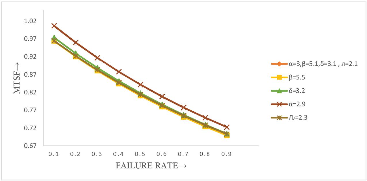
Figure 2 MTSF vs constant failure rate ($\lambda )$, repair rate ($\pi$), constant maintenance rate ($\alpha$), preventive maintenance rate ($\delta$), rest completion rate ($\beta$).

Table 2 Availability vs constant failure rate ($\lambda )$, repair rate $(\pi )$, constant maintenance rate ($\alpha$), preventive maintenance rate ($\delta$), rest completion rate ($\beta$)

	$\alpha =3,\beta =5.1,$
$\lambda$	$\delta =3.1,\pi =2.1$	$\beta =5.5$	$\delta =3.2$	$\alpha =2.9$	$\pi =2.3$
0.1	0.662463	0.662532	0.67267985	0.67326055	0.66346589
0.2	0.646351	0.646608	0.65632614	0.65681518	0.64845399
0.3	0.629478	0.630011	0.63916289	0.6395808	0.63272461
0.4	0.612086	0.612959	0.62144541	0.62180687	0.61647982
0.5	0.594385	0.595642	0.60339453	0.60370975	0.59989823
0.6	0.576555	0.578221	0.58519833	0.58547418	0.58313542
0.7	0.558746	0.560832	0.56701458	0.56725556	0.56632515
0.8	0.541082	0.543588	0.54897357	0.54918247	0.54958074
0.9	0.523664	0.52658	0.53118107	0.53135957	0.53299689

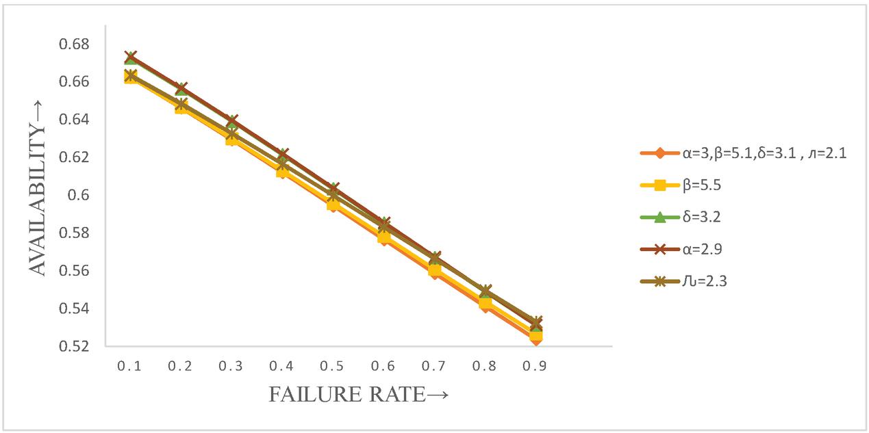
Figure 3 Availability MTSF vs constant failure rate ($\lambda )$, repair rate $(\pi )$, constant maintenance rate ($\alpha$), preventive maintenance rate ($\delta$), rest completion rate ($\beta$).

Table 3 Profit analysis vs constant failure rate ($\lambda )$, repair rate $(\pi )$, constant maintenance rate ($\alpha$), preventive maintenance rate ($\delta$), rest completion rate ($\beta$)

Let $K_0=15000,K_1=5000,K_2=3000,K_3=2000$ and $K_4=1000$
$\lambda$	$\alpha =3,\beta =5.1,\delta =3.1,\pi =2.1$	$\beta =5.5$	$\delta =3.2$	$\alpha =2.9$	$\pi =2.3$
0.1	7411.316	7408.477	7531.168	7608.732	7456.974
0.2	6590.387	6579.506	6702.449	6786.38	6686.794
0.3	5695.93	5672.399	5798.063	5893.162	5844.286
0.4	4751.857	4711.563	4842.563	4952.539	4950.468
0.5	3778.124	3717.388	3856.448	3984.092	4023.238
0.6	2791.163	2706.715	2856.604	3003.941	3077.652
0.7	1804.313	1693.277	1856.737	2025.163	2126.224
0.8	828.2337	688.1128	867.7929	1058.193	1179.211
0.9	-128.713	-300.041	-101.645	111.1986	244.8994

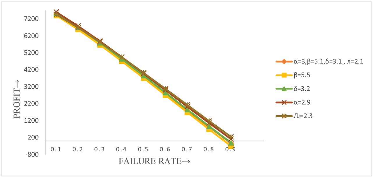
Figure 4 Profit analysis vs constant failure rate ($\lambda )$, repair rate $(\pi )$, constant maintenance rate ($\alpha$), preventive maintenance rate ($\delta$), rest completion rate ($\beta$) .

15 Real Life Application

The computer system can be considered as an example of the present work. In any workstation, suppose there is a full time need of computer system. Then we can have two computer systems, one is operative and other is kept as spare in cold standby in order to cover the risk or any emergency requirement. It is a matter of fact that every electronic system needs preventive maintenance after some specific period of operation. And, system will get repaired only when it completely fails. If, there is only a single server who immediately visits the workstation whenever needed, then if both operations preventive maintenance and repair of the computer system required at a time. Then server can give priority to preventive maintenance over repair. As maintenance requires less time and energy of the server and the computer system can be used again after maintenance. And, server does not need any rest after preventive maintenance. If both the computer systems fail, then after repairing one system, the server needs a rest to regain his energy for repairing the other unit of the system. After taking some rest, the server can do the assigned job of repairing the other system continuously with same enthusiasm.

16 Discussion and Conclusion

Here, in a two-unit cold standby system, the concept of rest of the server after each repair is implemented. The concept of preventive maintenance is also considered after specific period of operation. There is a single server who visits the system immediately whenever needed. Priority is given to preventive maintenances over repairs. The reliability traits MTSF, availability and eventually the profit function are obtained for arbitrary parameter values. It is noted that the mean time to system failure and system model availability continue to decrease with the increase in the unit’s failure rate, although their values continue to increase with the increase in the repair rate and the rate at which the server accomplishes the rest. The profit function of the system model also follows the same pattern for $K_0=15000,K_1=5000,K_2=3000,K_3=2000,K_4=1000$. Consequently, a system which provides the rest to the server between repair works can only make the system consistent and financially beneficial to use by increasing the rest completion rate of the server (may be called a technician). In Tables 1–3 and Figures 2–4, the findings of these measures are described numerically and graphically.

References

[1] Goel, L.R. and Shrivastava, P. (1991): A Two Unit Cold Standby System with Three Modes and Correlated Failures and Repairs, Microelectronics Reliability, Vol. 31(5), pp. 835–840.

[2] Gupta, R., Chaudhary, P. and Kumar D. (2007): Stochastic Analysis of a Two Unit Cold Standby System with Different Operative Modes and Different Repair Policies, International Journal of Agriculture Statistics Sciences, Vol. 3(2), pp. 387–394.

[3] Kumar, P. and Gupta, R. (2007). Reliability Analysis of a Single Unit M|G|1 System Model with Helping Unit. Journal of Combinatorics Information& System Sciences, Vol. 32, No. 1–4, pp. 209–219.

[4] Wu, Q. and Wu, S. (2011): Reliability Analysis of Two Unit Cold Standby Repairable Systems under Poisson Shocks, Applied Mathematics and Computation, Vol. 218(1), pp. 171–182.

[5] Wang, C., Xing, L. and Amari, S.V. (2012): A Fast Approximation Method for Reliability Analysis of Cold Standby Systems, Reliability Engineering & System Safety, Vol. 106, pp. 119–126.

[6] Kumar, D. and Singh, S.B. (2016): Stochastic Analysis of Complex Repairable System with Deliberate Failure Emphasizing Reboot Delay, Communications in Statistics – Simulation and Computation, Vol. 45(2), pp. 583–602.

[7] Lado, A.K., Singh, V.V., Ismail, K.H. and Ibrahim, Y. (2018): Performance and Cost Assessment of Repairable Complex System with Two Subsystems Connected in Series Configuration, International Journal of Reliability and Applications, Vol. 19(1), pp. 27–42.

[8] Goel, M. and Kumar, J. (2018): Stochastic Analysis of a Two Unit Cold Standby System with Preventive Maintenance and General Distribution of all Random Variables, International Journal of Statistics and Reliability Engineering, Vol. 5(1), pp. 10–21.

[9] Barak, M.S., Yadav D. and Barak S. (2018): Stochastic Analysis of two-unit Redundant System with Priority to Inspection over Repair, Life Cycle Reliability and Safety Engineering, Vol. 7, pp. 71–79.

[10] Kumar, A., Pawar, D. and Malik, S.C. (2019): Profit Analysis of a Warm Standby Non-Identical Units System with Single Server Subject to Preventive Maintenance. International Journal of Agricultural and Statistical Sciences, Vol. 15(1), pp. 261–269.

[11] Shinde, V., Biniwale, D. and Bharadwaj, S.K. (2019): Availability Analysis for Estimation of Repair Rate of Performance based Logistics under Operating Conditions, Journal of Reliability and Statistical Studies, Vol. 12(1), pp. 65–78.

[12] Lado, A.K. and Singh, V.V. (2019): Cost Assessment of Complex Repairable System consisting Two Subsystems in Series Configuration using Gumbel Hougaard family copula, International Journal of Quality Reliability and Management, Vol. 36(10), pp. 1683–1698.

[13] Aggarwal, C. and Malik, S.C. (2020): A Standby Repairable System with Rest of Server between Repairs, Journal of Statistics and Management Systems (online).

[14] Singh, V.V., Poonia, P.K. and Adbullahi, A.H. (2020): Performance Analysis of a Complex Repairable System with Two Subsystems in Series Configuration with an Imperfect Switch, Journal of Mathematical and Computational Science, Vol. 10(2), pp. 359–383.

[15] Raghav, D., Pooni, P.K., Gahlot, M., Singh, V.V., Ayagi, H.I. and Abdullahi, A.H. (2020): Probabilistic Analysis of a System Consisting of Two Subsystems in the Series Configuration under Copula Repair Approach, Journal of Korean Society of Mathematical Educational. Ser. B: The Pure and Applied Mathematics, Vol. 27(3), pp. 137–155.

Biographies

Chhama Aggarwal is a Ph.D. student at the Department of Statistics in Maharshi Dayanand University since October, 2018. She received her B.Sc. (H) Mathematics and M.Sc. in Mathematics degrees from University of Delhi, Delhi.

Nitika Ahlawat is a Ph.D. student at the Department of Statistics in Maharshi Dayanand University since December, 2019. She received her B.A. in Mathematics and Statistics and M.Sc. in Statistics degrees from M.D. University, Rohtak (Haryana).

S. C. Malik is presently working as Professor & Head, Department of Statistics, M.D. University, Rohtak (Haryana). His field of research specialization are Reliability Theory, Sampling and Applied Statistics. He has a long research and teaching experience in subject of Statistics. He has supervised 40 Ph.D. students in the fields of reliability theory, sampling theory and applied statistics. Dr. Malik has been invited by various academic institutions to deliver talks and to present research papers at conferences/seminars/symposiums/workshops held in India and abroad including USA, UK, Portugal, Singapore, Germany, Hong-Kong, France, Spain, Netherland, Belgium, Austria, Italy, Japan, Switzerland and Nepal. He is reviewer of various journals specifically for the journals in the areas of Reliability, Operations Research and Statistics. Prof. Malik has been a member/life member of various academic/professional bodies. He is a founder President of Indian Association for Reliability and Statistics (IARS) and also Chief Editor of the UGC listed journal IJSRE being published by IARS.

Journal of Reliability and Statistical Studies, Vol. 14, Issue 1 (2021), 57–80.
doi: 10.13052/jrss0974-8024.1414
© 2021 River Publishers

Abstract

1 Introduction

2 Notations

3 System Description

4 Transition Probabilities

5 Mean Sojourn Time

6 Mean Time to System Failure (MTSF)

7 Availability Analysis

8 Busy Period Analysis of the Server Due to Repair

9 Busy Period Analysis of The Server Due to Preventive Maintenance

10 Expected Number of Repairs

11 Expected Number of Preventive Maintenances

12 Profit Analysis

13 Particular Case

14 Numerical and Graphical Representation Of Different Reliability Measures

15 Real Life Application

16 Discussion and Conclusion

References

Biographies