Reliability Evaluation of Repairable Parallel-Series Multi-State System Implementing Interval Valued Universal Generating Function

Renu¹, Soni Bisht^2,* and S. B. Singh¹

¹Department of Mathematics, Statistics and Computer Science, G.B. Pant University of Agriculture and Technology, Pantnagar, India

²Department of Mathematics, Eternal University, Baru Sahib, Himachal Pradesh, India

E-mail: renutamta17@gmail.com; bsdipi1992@gmail.com; drsurajbsingh@yahoo.com

*Corresponding Author

Received 12 October 2020; Accepted 11 January 2021; Publication 22 March 2021

Abstract

In this paper, we have studied a repairable parallel-series multi-state system. The proposed system consists of m components in series and n components in parallel in which each component has three possible states. The interval universal generating function (IUGF) is presented, and the corresponding composition operators are defined. The reliability assessment of the considered system is done with the help of the IUGF approach. It is worth mentioning that IUGF got attention from various researchers due to its straightforwardness, less complexity, and universal applications. In the present model, probabilities of different components, reliability, sensitivity, and mean time to failure are evaluated with the help of the Markov process; Laplace-Steiltjes transform method applying IUGF. A numerical example has also been taken to illustrate the proposed technique.

Keywords: Interval valued universal generating function, repairable parallel-series multi-state system, reliability, sensitivity, mean-time-to-failure, Laplace-Steiltjes transform.

1 Introduction

If any equipment is found reliable based on the quality of its components and experiences of users, it means their performance is free from disturbances to a great extent, though its failure may not be completely ruled out. In other words, we can say that a certain degree of uncertainty in components performance may be involved. Kozin and Utkin (2002) introduced the concept of interval-valued coherent previsions to generalize the discrete-Markov chains to the interval-valued probabilities. Xiaoping (2007) investigated the reliability characteristics corresponding to the random and intervals inputs for black-box function and nonlinear optimization. An engineering example has also been illustrated. Zon et al. (2008) considered a discrete stress-strength interference model with the application of the universal generating function (UGF). Gupta et al. (2009) evaluated the reliability of the series system under restricted redundancy allocation. Authors illustrated their work by considering some series of redundancy allocation problems and examining the sensitivity of the systems with respect to different parameters. Li et al. (2011) analyzed the interval universal generating function (IUGF) and corresponding operators multi-state systems (MSSs) of having insufficient available data. In this study, they discussed the reliability of the system and affine arithmetic to improve interval-valued reliability using the imprecise Dirichlet model and Bayesian approach. Lisnianski et al. (2009) considered redundancy in two interconnected repairable MSSs and developed a method to compute the reliability based on UGF and random process. Yong, et al. (2012) extended the effects of uncertainty in system reliability and load demand on the system reliability. Subsequently, these two sets of uncertainty factors are estimated through UGF in repeated form. They applied this to MSSs of a multi-state series-parallel system. Ram and Singh (2012) presented a system having two independent repairable subunits and considered the Head-of-Line repair scheme. The Laplace transformation (LT) and Gumbel-Hougaard (G-H) family of copula were used by the authors to analyze the state transition probabilities and reliability of the system. Kumar and Singh (2013) considered a complex system, in which the subsystems A and B are joined in series while subsystem A is of k-out-of-n: G configuration and B is of circular consecutive 2-out-of 3: F configuration. With the LT and G-H family of the copula, the researchers analyzed the reliability, state transition probabilities, availability, cost analysis, and MTTF of the system. Xing et al. (2013) proposed the binary decision diagrams-based method for the reliability evaluation of non-repairable binary-state phased mission with common cause failure. Here, authors designed a combinatorial algorithm based on a binary decision diagram. Wang et al. (2013) studied the repairable system to examine the reliability characteristics incorporating imperfect coverage and service pressure condition. Here, authors also discussed the effects of different parameters on system reliability and MTTF. Jain and Gupta (2013) developed a mathematical model for a repairable structure incorporating a single repairman with multiple vacations. They evaluated the reliability characteristics with the use of supplementary variable technique, exponential distribution, and Laplace transformation. Guilani et al. (2014) computed the reliability of the three-state non-repairable system through the Markov process and compared the results with the UGF method. Pokoradi (2014) investigated the adaption of mathematical diagnostic of aircraft systems and gas turbine engines to compute the sensitivity of the reliability of finite system having complex interconnections. Wu et al. (2014) examined a repairable system with k-out of-n: G configuration having one repairman with only one vacation which follows an exponential distribution. Each component’s working time is exponentially distributed, and the repair time of each failed component is arbitrarily distributed. They evaluated the various reliability characteristics, namely, MTTF, availability, and rate of occurrence of a failure with LT and supplementary variable technique (SVT). Levitin et al. (2014) presented the non-repairable system with l-out-of-N configuration, with sufficient choice of the load which affected the lifetime acceleration factor, operational and replacement costs. The authors focused on the standby system’s optimal load distribution problem and minimized the mission cost under reliability restrictions. Cekyay and Ozekici (2015) studied the coherent system in which the series connection of u-out-of-v standby subsystem with exponentially distributed component and evaluated the reliability characteristics. Negi and Singh (2015) computed reliability, MTTF, and sensitivity of a complex system having non-repairable weighted u-out-of-v: G connected in series with linear-$(k,f,e)$: G and circular-$(k,f,e)$: G configuration based on UGF. Wang et al. (2016) analyzed the reliability optimization of a heterogeneous cold-standby system having uncertainty in parameter, compared interval numbers and provided an algorithm to evaluate the system reliability and expected mission cost using IUGF. Pan et al. (2016) formed a distribution scheme using an interval parameter for the estimation of system reliability with the help of improved UGF and IUGF methods. Xu et al. (2016) investigated the dynamic diagnosis method, which is based on interval-valued belief structures. Here, the authors also analyzed the reliability characteristics of the considered system. They also compared the performance of the proposed updating strategy with traditional strategies. Kumar et al. (2016) studied the reliability of a 2-out-of-4 system using IUGF. To illustrate the model, a numerical problem has also been discussed. Meenakshi and Singh (2016) discussed the reliability of non-repairable MSSs with imprecise probabilities and performance rates having interval-valued probabilities with the use of hybrid UGF.

The present paper is arranged as follows. Section 1 includes definitions of the proposed model and estimation of state probabilities of MSSs component based on the Markov process. In Sections 2 and 3, we calculate the interval-valued system reliability of the considered MSSs. After that, a numerical example is taken, which illustrates the proposed method in Section 4. In Section 5, the numerical results of the supposed system were discussed. Finally, the conclusion is given in Section 6. The proposed system is shown in Figure 1. The notations used in the study have been listed in Table 1.

Table 1 Notations

C${}_i$	Component of a system, where $i=1,2,3,\mathrm{\dots }N$
N	Total number of components in the system
g${}_i$	Performance level of the component for the state i
${\underset{¯}{p}}_i,{\overline{p}}_i$	Lower and upper bound of the probability of $i$th component state
$u_i(z)$	IUGF of component i
$u(z)$	IUGF of system
$\underset{ser}{\otimes }$	Composition operator to be used in series combination
$\underset{par}{\otimes }$	Composition operator to be used in parallel combination
W	The required performance level of the system
${\underset{¯}{\lambda }}_{ij}$,${\overline{\lambda }}_{ij}$	Lower and upper bound of the failure rate of the component for the transition from $i$th component state to $j$th component state
${\underset{¯}{\mu }}_{ij}$	Upper bound of repair rate of the component for the transition from $i$th component state to $j$th component state
$[R]$	Reliability of the system

2 Definitions

2.1 Universal Generating Function (UGF)

UGF is a widely used approach to estimate the reliability of the various systems. This method is firstly introduced by Ushakov in 1986.

2.2 Probability Intervals

In the face of uncertainties of different kinds, probability intervals are used for making qualitative and quantitative estimates. It is used, through mathematical expressions, to find partial information about random variables and other quantities. Probability intervals are limited to input distributions, without requiring more precise parameter value knowledge. Let $C_i$ be any component in repairable parallel-series MSSs consisting of m components in series and n components in parallel and $p_j$ be the probability of state j, where $j=1,2,3$ denotes the number of states of the components in the system. Let ${\lambda }_{jk}$ and ${\mu }_{jk}$ be the degradation rate and repair rate respectively, where j is the upper state and k is any lower state that lies in the interval [${\underset{¯}{\lambda }}_{jk},{\overline{\lambda }}_{jk}$] and [${\underset{¯}{\mu }}_{jk},{\overline{\mu }}_{jk}$] respectively. The following set of differential equations governing the behavior of the system based on a stochastic process using interval-valued parameters can be obtained:

$f_j(p,\lambda ,\mu ,t)$	$={\displaystyle \frac{d{p}_j(t)}{dt}}={\displaystyle \sum _{k=j+1}^j}{\lambda }_{kj}{p}_k(t)$
	$\mathrm{\hspace{1em}}+{\displaystyle \sum _{k=1}^{j-1}}{\mu }_{kj}{p}_k(t)-p_j(t)\left({\displaystyle \sum _{k=1}^{j-1}}{\lambda }_{jk}+{\displaystyle \sum _{k=j+1}^j}{\mu }_{jk}\right)$	(1)

Lower and upper probability bounds of the system are calculated as:

$$\frac{\partial f_j(p,\lambda ,\mu ,t)}{\partial P_j(t)}\ge 0,\forall j,k,$$
$$\forall {\lambda }_{jk}\in [{\underset{¯}{\lambda }}_{jk},{\overline{\lambda }}_{jk}],{\lambda }_{kj}\in [{\underset{¯}{\lambda }}_{kj},{\overline{\lambda }}_{kj}],\forall {\mu }_{jk}\in [{\underset{¯}{\mu }}_{jk},{\overline{\mu }}_{jk}],$$
$${\mu }_{kj}\in [{\underset{¯}{\mu }}_{kj},{\overline{\mu }}_{kj}],k\ne i,t\ne t_0$$	(2)
$$\text{If }\frac{\partial f_j(p,\lambda ,\mu ,t)}{\partial {\lambda }_j(t)}\ge 0,\forall t>0,\text{then }{\mu }_{kj}={\underset{¯}{\mu }}_{kj},{\lambda }_{kj}={\underset{¯}{\lambda }}_{kj}$$	(3)
$$\text{If }\frac{\partial f_j(p,\lambda ,\mu ,t)}{\partial {\lambda }_j(t)}\le 0,\forall t>0,\text{then }{\mu }_{kj}={\overline{\mu }}_{kj},{\lambda }_{kj}={\overline{\lambda }}_{kj}$$	(4)

Using Equations (3)–(4) in Equation (1) one can compute lower bound of probability as:

${\displaystyle \frac{d{\underset{¯}{p}}_j(t)}{dt}}$	$={\displaystyle \sum _{k=j+1}^j}{\underset{¯}{\lambda }}_{kj}{\underset{¯}{p}}_k(t)+{\displaystyle \sum _{k=1}^{j-1}}{\underset{¯}{\mu }}_{kj}{\underset{¯}{p}}_k(t)-{\underset{¯}{p}}_j(t)$
	$\mathrm{\hspace{1em}}\times \left({\displaystyle \sum _{k=1}^{j-1}}{\overline{\lambda }}_{jk}+{\displaystyle \sum _{k=j+1}^j}{\overline{\mu }}_{jk}\right),$	(5)

Similarly, the upper bound of the probability of the system can be computed by using Equations (6)–(7).

$\text{If }{\displaystyle \frac{\partial f_j(p,\lambda ,\mu ,t)}{\partial {\lambda }_j(t)}}\ge 0,\forall t>0,\text{then }{\mu }_{kj}={\overline{\mu }}_{kj},{\lambda }_{kj}={\overline{\lambda }}_{kj}$	(6)
$\text{If }{\displaystyle \frac{\partial f_j(p,\lambda ,\mu ,t)}{\partial {\lambda }_j(t)}}\le 0,\forall t>0,\text{then }{\mu }_{kj}={\underset{¯}{\mu }}_{kj},{\lambda }_{kj}={\underset{¯}{\lambda }}_{kj}$	(7)

Applying Equations (6)–(7) in Equation (2), upper bound probability can be computed as

${\displaystyle \frac{d{\overline{p}}_j(t)}{dt}}$	$={\displaystyle \sum _{k=j+1}^j}{\overline{\lambda }}_{kj}{\overline{p}}_k(t)+{\displaystyle \sum _{k=1}^{j-1}}{\overline{\mu }}_{kj}{\overline{p}}_k(t)-{\overline{p}}_j(t)$
	$\mathrm{\hspace{1em}}\times \left({\displaystyle \sum _{k=1}^{j-1}}{\underset{¯}{\lambda }}_{jk}+{\displaystyle \sum _{k=j+1}^j}{\underset{¯}{\mu }}_{jk}\right),$	(8)

Lower and upper bound probabilities can be evaluated by using Equations (5)–(8), with the help of Laplace-Steiltjes transform.

2.3 Interval Universal Generating Function

In the system reliability assessment, one of the factors is to deal with uncertainty that occurs in the system modeling, data etc. There are difficulties that may be due to the lack of information that results in data uncertainty. For uncertainty representation and utilization in availability assessment, the IUGF approach can be used. Foundation of IUGF is laid by UGF and probability intervals.

The IUGF of a component $G^j$ with $M_j$ states is expressed as:

$$U_j=\sum _{i=1}^{M_j}[p_i^j]z^{g_i^j}$$

(9)

2.4 Composition Operator

An interval valued number I is an uncertain number and defined as:

$I=[i_L,i_R]=\{i_L\le i\le i_R,i\in R\}$

(10)

If $i_L=i=i_R$ then $I$ is said to be a point interval and expressed as

$i=[\mathit{\text{i}},\mathit{\text{i}}].$

(11)

If we have two interval numbers $S=[s_L,s_R]$ and $T=[S_L,T_R]$, where $s_L\ge 0$, and $t_L\ge 0$ then basic arithmetical operations of interval variables are defined as:

(i) Addition

$$S+T=[s_L+t_L,s_R+t_R]$$

(12)

(ii) Subtraction

$$S-T=[s_L-t_R,s_R-t_L]$$

(13)

(iii) Multiplication

$$\mathit{\text{ST}}=[s_L{t}_L,s_R{t}_R]$$

(14)

(iv) Division

$S/T=[{\displaystyle \frac{s_L}{t_R}},{\displaystyle \frac{s_R}{t_L}}]$

(15)

With the help of Equation (9), IUGF of considered model having m states is defined as:

$U_c(z)={\displaystyle \sum _{i=1}^m}[{\underset{¯}{p}}_i,{\overline{p}}_i]z^{g_i}$

(16)

Corresponding to the component’s configuration in the MSSs, the IUGF is defined as:

(i) If n components of the system are in series combination, then the IUGF of the system is given by:

$(U_1(z)\underset{ser}{\otimes },\mathrm{\dots },\underset{ser}{\otimes }{U}_n(z))$
$\mathrm{\hspace{1em}\hspace{1em}}={\displaystyle \sum _{l_1=1}^{k_1}}\mathrm{\dots }{\displaystyle \sum _{l_n=1}^{k_n}}[{\displaystyle \prod {}_{i=1}{}^n\underset{¯}{p}_{l_i}^i},{\displaystyle \prod _{i=1}^n}{\overline{p}}_{l_i}^i]z^{(\min (g_{l_1}^1,\mathrm{\dots },g_{l_n}^n))}$	(17)

(ii) If n components of the system are in parallel combination, then the IUGF of the system is expressed as:

$(U_1(z)\underset{par}{\otimes },\mathrm{\dots },\underset{par}{\otimes }{U}_n(z))$
$\mathrm{\hspace{1em}\hspace{1em}}={\displaystyle \sum _{l_1=1}^{k_1}}\mathrm{\dots }{\displaystyle \sum _{l_n=1}^{k_n}}[{\displaystyle \prod _{i=1}^n}{\underset{¯}{p}}_{l_i}^i,{\displaystyle \prod _{i=1}^n}{\overline{p}}_{l_i}^i]z^{(\max (g_{l_1}^1,\mathrm{\dots },g_{l_n}^n)}$	(18)

Consider a parallel-series system consisting of m components in series and n components in parallel combination. Suppose there are three different states for each component of the considered system. It is assumed that the failure and repair rates are having equal values for the same components states for each component in the proposed system. The IUGF of each component is expressed as:

$u_{c_1}(z)$	$=[{\underset{¯}{p}}_3,{\overline{p}}_3]z^{g_3^1}+[{\underset{¯}{p}}_2,{\overline{p}}_2]z^{g_2^1}+[{\underset{¯}{p}}_1^1,{\overline{p}}_1]z^{g_1^1}$	(19)
$u_{c_2}(z)$	$=[{\underset{¯}{p}}_3,{\overline{p}}_3]z^{g_3^2}+[{\underset{¯}{p}}_2,{\overline{p}}_2]z^{g_2^2}+[{\underset{¯}{p}}_1^1,{\overline{p}}_1]z^{g_1^2}$	(20)
	$\mathrm{⋮}$
$u_{c_{mn}}(z)$	$=[{\underset{¯}{p}}_3,\overline{p_3}]z^{g_3^{mn}}+[{\underset{¯}{p}}_2,\overline{p_2}]z^{g_2^{mn}}+[{\underset{¯}{p^1}}_1,\overline{p_1}]z^{g_1^{mn}}$	(21)

Let $C_1,C_2,\mathrm{\dots }$ and $C_m$ be arranged in series combination in the system, then IUGF of $C_1,C_2,\mathrm{\dots }$ and $C_m$ is given by:

$u_{c_1,c_2\mathrm{\dots }{c}_m}(z)$	$=u_{c_1}(z)\underset{ser}{\otimes }{u}_{c_2}(z)\mathrm{\dots }\underset{ser}{\otimes }{u}_{c_m}(z)$
	$=[{({\underset{¯}{p}}_3)}^m,{(\overline{p_3})}^m]z^{\min (g_3^1,g_3^2\mathrm{\dots }{g}_3^m)}$
	$\mathrm{\hspace{1em}}+[{({\underset{¯}{p}}_2)}^m,{(\overline{p_2})}^m]z^{\min (g_2^1,g_2^2\mathrm{\dots }{g}_2^m)}\mathrm{\dots }[{({\underset{¯}{p}}_1)}^m,{(\overline{p_1})}^m]$
	$\mathrm{\hspace{1em}}{z}^{\min (g_1^1,g_1^2\mathrm{\dots }{g}_1^m)}$	(22)

Since n components are in parallel combination, therefore IUGF of the considered system is articulated as:

$u_{sys}(z)$	$=\underset{par}{\overset{i=1}{\otimes }}\{u_{c_1}(z)\underset{ser}{\otimes }{u}_{c_2}(z)\underset{ser}{\otimes }\mathrm{\dots }\underset{ser}{\otimes }{u}_{c_m}(z)\}$
	$=[{({\underset{¯}{p}}_3)}^{m(1+n)},{({\overline{p}}_3)}^{m(1+n)}]z^{\min (g_3^1,g_3^2\mathrm{\dots }.g_3^m)}$
	$\mathrm{\hspace{1em}}+{({\underset{¯}{p}}_2)}^m,{({\underset{¯}{p}}_3)}^{mn},{({\overline{p}}_2)}^m,{({\underset{¯}{p}}_3)}^{mn}]$
	$\mathrm{\hspace{1em}}{z}^{\max \{\min (g_2^1,g_2^2\mathrm{\dots }.g_2^m)\min (g_3^1,g_3^2\mathrm{\dots }.g_3^m)\}}$
	$\mathrm{\hspace{1em}}+{({\underset{¯}{p}}_1)}^m,{({\underset{¯}{p}}_3)}^{mn},{({\overline{p}}_1)}^m,{({\underset{¯}{p}}_3)}^{mn}]$
	$\mathrm{\hspace{1em}}{z}^{\max \{\min (g_1^1,g_1^2\mathrm{\dots }.g_1^m)\min (g_3^1,g_3^2\mathrm{\dots }.g_3^m)\}}$	(23)

2.5 Interval Valued System Reliability of Repairable MSS

In the considered parallel-series multi state system, there are m and n components in series and parallel combination respectively. Let the interval-valued state performance levels and state probabilities of the MSSs be $g_j,g_j,g_j,\mathrm{\dots },g_j$ and $P_j,P_j,P_j,\mathrm{\dots },P_j$ respectively, where $j=1,2,3$.

If demand level is w, then the system interval valued reliability [R] of MSSs is computed as:

$$[R]=\sum _{i=1}^R[p_i|r_i\ge w]$$

(24)

3 Algorithm for Computing the System Interval Valued Reliability

Step-1: Determine IUGF of each element with the help of equation (16).

Step-2: Assign $R=0$, $U_1(z)=u_1(z)$.

Step-3: For $j=2,3\mathrm{\dots },\mathit{\text{n}}$

$$U_j(z)=U_{j-1}(z)\otimes U_j(z).$$

Step-4: Evaluate probability intervals from Equations (5) and (8) using Laplace-Steiltjes transform for each component state of each system component.

Step-5: Set demand level w and compute the system interval valued reliability [R] of MSSs using Equation (24)

$$[R]=\sum _{i=1}^R[p_i|r_i\ge w]$$

4 Numerical Example

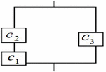
Consider a repairable parallel-series multi-state system having three components $c_1,c_2$, and $c_3$ Let each component has three possible states corresponding to their performance rates. Figure 1 represents the considered system.

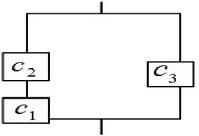
Figure 1 Repairable parallel-series system.

Let us presume that the failure and repair rates of all three system components have the same values for the same component states, respectively, for the system considered. Let the failure and repair rates of the repairable multi-state parallel-series system be ${\underset{¯}{\lambda }}_{32}=0.09,{\overline{\lambda }}_{32}=0.1,{\underset{¯}{\lambda }}_{21}=0.02,{\overline{\lambda }}_{21}=0.025$ and ${\underset{¯}{\mu }}_{12}=0.025,{\overline{\mu }}_{12}=0.03$ respectively.

By applying Equation (5), we get following differential equations for lower bound probabilities of components of the system at time t:

${\displaystyle \frac{d\underset{¯}{p_1}(t)}{dt}}$	$=-\overline{{\mu }_{12}}\underset{¯}{p_1}(t)+\underset{¯}{{\lambda }_{21}}\underset{¯}{p_2}(t)$	(25)
${\displaystyle \frac{d\underset{¯}{p_2}(t)}{dt}}$	$=-\overline{{\lambda }_{21}}\underset{¯}{p_2}(t)+\underset{¯}{{\mu }_{12}}\underset{¯}{p_1}(t)+\underset{¯}{{\lambda }_{32}}\underset{¯}{p_3}(t)$	(26)
${\displaystyle \frac{d\underset{¯}{p_3}(t)}{dt}}$	$=-\overline{{\lambda }_{32}}\underset{¯}{p_3}(t)$	(27)

Initial condition: $p_3(t)=1$ at $t=0$ and all other probabilities are zero initially.

Solving Equations (25)–(27), we get lower bound probabilities as:

$\underset{¯}{p_1}(t)$	$=-{\displaystyle \frac{\underset{¯}{{\lambda }_{21}}\underset{¯}{{\lambda }_{32}}}{(\overline{{\mu }_{12}}+\overline{{\lambda }_{21}}-\overline{{\lambda }_{32}})\overline{{\lambda }_{32}}-\overline{{\lambda }_{21}}\overline{{\mu }_{12}}+\underset{¯}{{\lambda }_{21}}\underset{¯}{{\mu }_{12}}}}[e^{-(\overline{{\lambda }_{32}}t)}+e^{-\frac{\overline{({\mu }_{12}}+\overline{{\lambda }_{21})}}{2}t}$
	$\mathrm{\hspace{1em}}\{{\displaystyle \frac{\overline{{\mu }_{12}}+\overline{{\lambda }_{21}}}{\sqrt{{(\overline{{\mu }_{12}}-\overline{{\lambda }_{21}})}^2+\underset{¯}{{\lambda }_{21}}\underset{¯}{{\mu }_{12}}}}}\sinh \left({\displaystyle \frac{t}{2}}\sqrt{{(\overline{{\mu }_{12}}-\overline{{\lambda }_{21}})}^2+\underset{¯}{{\lambda }_{21}}\underset{¯}{{\mu }_{12}}}\right)$
	$\mathrm{\hspace{1em}}-\cosh \left({\displaystyle \frac{t}{2}}\sqrt{{(\overline{{\mu }_{12}}-\overline{{\lambda }_{21}})}^2+\underset{¯}{{\lambda }_{21}}\underset{¯}{{\mu }_{12}}}\right)\}]$
	$\mathrm{\hspace{1em}}+e^{-\frac{\overline{({\mu }_{12}}+\overline{{\lambda }_{21})}}{2}t}{\displaystyle \frac{\sinh \left(\frac{t}{2}\sqrt{{(\overline{{\mu }_{12}}-\overline{{\lambda }_{21}})}^2+\underset{¯}{{\lambda }_{21}}\underset{¯}{{\mu }_{12}}}\right)}{\sqrt{{(\overline{{\mu }_{12}}-\overline{{\lambda }_{21}})}^2+\underset{¯}{{\lambda }_{21}}\underset{¯}{{\mu }_{12}}}}}$
	$\mathrm{\hspace{1em}}\times \left[{\displaystyle \frac{\underset{¯}{{\lambda }_{21}}\underset{¯}{{\lambda }_{32}}}{(\overline{{\mu }_{12}}+\overline{{\lambda }_{21}}-\overline{{\lambda }_{32}})\overline{{\lambda }_{32}}-\overline{{\lambda }_{21}}\overline{{\mu }_{12}}+\underset{¯}{{\lambda }_{21}}\underset{¯}{{\mu }_{12}}}}(\overline{{\mu }_{12}}+\overline{{\lambda }_{21}}-\overline{{\lambda }_{32}})\right]$	(28)
$\underset{¯}{p_2}(t)$	$=-{\displaystyle \frac{{(\underset{¯}{{\lambda }_{32}})}^2-\underset{¯}{{\mu }_{21}}\underset{¯}{{\lambda }_{32}}}{(\overline{{\mu }_{12}}+\overline{{\lambda }_{21}}-\overline{{\lambda }_{32}})\overline{{\lambda }_{32}}-\overline{{\lambda }_{21}}\overline{{\mu }_{12}}+\underset{¯}{{\lambda }_{21}}\underset{¯}{{\mu }_{12}}}}[e^{-(\overline{{\lambda }_{32}}t)}+e^{-\frac{\overline{({\mu }_{12}}+\overline{{\lambda }_{21})}}{2}t}$
	$\mathrm{\hspace{1em}}\times \{{\displaystyle \frac{\overline{{\mu }_{12}}+\overline{{\lambda }_{21}}}{\sqrt{{(\overline{{\mu }_{12}}-\overline{{\lambda }_{21}})}^2+\underset{¯}{{\lambda }_{21}}\underset{¯}{{\mu }_{12}}}}}\sinh \left({\displaystyle \frac{t}{2}}\sqrt{{(\overline{{\mu }_{12}}-\overline{{\lambda }_{21}})}^2+\underset{¯}{{\lambda }_{21}}\underset{¯}{{\mu }_{12}}}\right)$
	$\mathrm{\hspace{1em}}-\cosh \left({\displaystyle \frac{t}{2}}\sqrt{{(\overline{{\mu }_{12}}-\overline{{\lambda }_{21}})}^2+\underset{¯}{{\lambda }_{21}}\underset{¯}{{\mu }_{12}}}\right)\}]$
	$\mathrm{\hspace{1em}}+e^{-\frac{\overline{({\mu }_{12}}+\overline{{\lambda }_{21})}}{2}t}{\displaystyle \frac{\sinh \left(\frac{t}{2}\sqrt{{(\overline{{\mu }_{12}}-\overline{{\lambda }_{21}})}^2+\underset{¯}{{\lambda }_{21}}\underset{¯}{{\mu }_{12}}}\right)}{\sqrt{{(\overline{{\mu }_{12}}-\overline{{\lambda }_{21}})}^2+\underset{¯}{{\lambda }_{21}}\underset{¯}{{\mu }_{12}}}}}$
	$\mathrm{\hspace{1em}}\times \left[{\displaystyle \frac{{\left(\underset{¯}{{\lambda }_{32}}\right)}^2-\underset{¯}{{\mu }_{21}}\underset{¯}{{\lambda }_{32}}}{(\overline{{\mu }_{12}}+\overline{{\lambda }_{21}}-\overline{{\lambda }_{32}})\overline{{\lambda }_{32}}-\overline{{\lambda }_{21}}\overline{{\mu }_{12}}+\underset{¯}{{\lambda }_{21}}\underset{¯}{{\mu }_{12}}}}(\overline{{\mu }_{12}}+\overline{{\lambda }_{21}}-\overline{{\lambda }_{32}})\right]$	(29)
$\underset{¯}{p_3}(t)$	$=e^{-(\overline{{\lambda }_{32}}t)}$	(30)

Now using Equation (8), upper bound probabilities of the considered system can be obtained as

${\displaystyle \frac{d\overline{p_1}(t)}{dt}}$	$=-\underset{¯}{{\mu }_{12}}\overline{p_1}(t)+{\underset{¯}{\lambda }}_{21}\overline{p_2}(t)$	(31)
${\displaystyle \frac{d\overline{p_2}(t)}{dt}}$	$=-{\underset{¯}{\lambda }}_{21}\overline{p_2}(t)+{\overline{\mu }}_{12}\overline{p_1}(t)+{\overline{\lambda }}_{32}\overline{p_3}(t)$	(32)
${\displaystyle \frac{d{\overline{p}}_3(t)}{dt}}$	$=-{\underset{¯}{\lambda }}_{32}{\overline{p}}_3(t)$	(33)

Solving Equations (31)–(33), we have the upper bound probabilities are as:

$\overline{p_1}(t)$	$={\displaystyle \frac{-\overline{{\lambda }_{21}}\overline{{\lambda }_{32}}}{(\underset{¯}{{\mu }_{12}}+\underset{¯}{{\lambda }_{21}}-\underset{¯}{{\lambda }_{32}})\underset{¯}{{\lambda }_{32}}-\underset{¯}{{\lambda }_{21}}\underset{¯}{{\mu }_{12}}+\overline{{\lambda }_{21}}\overline{{\mu }_{12}}}}[e^{-(\underset{¯}{{\lambda }_{32}}t)}+e^{-\frac{(\underset{¯}{{\mu }_{12}}+\underset{¯}{{\lambda }_{21}})}{2}t}$
	$\mathrm{\hspace{1em}}\times \{{\displaystyle \frac{\underset{¯}{{\mu }_{12}}+\underset{¯}{{\lambda }_{21}}}{\sqrt{\underset{¯}{({\mu }_{12}}-{\underset{¯}{{\lambda }_{21})}}^2+4\overline{{\lambda }_{21}}\overline{{\mu }_{12}}}}}\sinh \left({\displaystyle \frac{t}{2}}\sqrt{\underset{¯}{({\mu }_{12}}-{\underset{¯}{{\lambda }_{21})}}^2+4\overline{\lambda {}_{21}^i}\overline{{\mu }_{12}^i}}\right)$
	$\mathrm{\hspace{1em}}-\cosh \left({\displaystyle \frac{t}{2}}\sqrt{\underset{¯}{({\mu }_{12}}-{\underset{¯}{{\lambda }_{21})}}^2+4\overline{{\lambda }_{21}^i}\overline{{\mu }_{12}^i}}\right)\}]$
	$\mathrm{\hspace{1em}}+e^{-\frac{(\underset{¯}{{\mu }_{12}}+\underset{¯}{{\lambda }_{21}})}{2}t}{\displaystyle \frac{\sinh \left(\frac{t}{2}\sqrt{\underset{¯}{({\mu }_{12}}-{\underset{¯}{{\lambda }_{21})}}^2+4\overline{{\lambda }_{21}}\overline{{\mu }_{12}}}\right)}{2\sqrt{\underset{¯}{({\mu }_{12}}-{\underset{¯}{{\lambda }_{21})}}^2+4\overline{{\lambda }_{21}}\overline{{\mu }_{12}}}}}$
	$\mathrm{\hspace{1em}}\times \left[{\displaystyle \frac{\overline{{\lambda }_{21}}\overline{{\lambda }_{32}}}{(\underset{¯}{{\mu }_{12}}+\underset{¯}{{\lambda }_{21}}-\underset{¯}{{\lambda }_{32}})\underset{¯}{{\lambda }_{32}}-\underset{¯}{{\lambda }_{21}}\underset{¯}{{\mu }_{12}}+\overline{{\lambda }_{21}}\overline{{\mu }_{12}}}}(\underset{¯}{{\mu }_{12}}+\underset{¯}{{\lambda }_{21}}-\underset{¯}{{\lambda }_{32}})\right]$	(34)
$\overline{p_2}(t)$	$={\displaystyle \frac{{(\overline{{\lambda }_{32}})}^2-\underset{¯}{{\mu }_{12}}\overline{{\lambda }_{32}}}{(\underset{¯}{{\mu }_{12}}+\underset{¯}{{\lambda }_{21}}-\underset{¯}{{\lambda }_{32}})\underset{¯}{{\lambda }_{32}}-\underset{¯}{{\lambda }_{21}}\underset{¯}{{\mu }_{12}}+\overline{{\lambda }_{21}}\overline{{\mu }_{12}}}}[e^{-(\underset{¯}{{\lambda }_{32}}t)}+e^{-\frac{\underset{¯}{({\mu }_{12}}+\underset{¯}{{\lambda }_{21})}}{2}t}$
	$\mathrm{\hspace{1em}}\times \{{\displaystyle \frac{\underset{¯}{({\mu }_{12}}+\underset{¯}{{\lambda }_{21})}}{\sqrt{\underset{¯}{({\mu }_{12}}-{\underset{¯}{{\lambda }_{21})}}^2+4\overline{{\lambda }_{21}}\overline{{\mu }_{12}}}}}\sinh \left({\displaystyle \frac{t}{2}}\sqrt{\underset{¯}{({\mu }_{12}}-{\underset{¯}{{\lambda }_{21})}}^2+4\overline{\lambda {}_{21}}\overline{{\mu }_{12}}}\right)$
	$\mathrm{\hspace{1em}}-\cosh \left({\displaystyle \frac{t}{2}}\sqrt{\underset{¯}{({\mu }_{12}}-{\underset{¯}{{\lambda }_{21})}}^2+4\overline{{\lambda }_{21}}\overline{{\mu }_{12}}}\right)\}]$
	$\mathrm{\hspace{1em}}+e^{-\frac{\underset{¯}{({\mu }_{12}}+\underset{¯}{{\lambda }_{21})}}{2}t}{\displaystyle \frac{\sinh \left(\frac{t}{2}\sqrt{\underset{¯}{({\mu }_{12}}-{\underset{¯}{{\lambda }_{21})}}^2+4\overline{{\lambda }_{21}}\overline{{\mu }_{12}}}\right)}{\sqrt{\frac{\underset{¯}{({\mu }_{12}}+{\underset{¯}{{\lambda }_{21})}}^2}{4}-\underset{¯}{{\lambda }_{21}}\underset{¯}{{\mu }_{12}}+\overline{{\lambda }_{21}}\overline{{\mu }_{12}}}}}$
	$\mathrm{\hspace{1em}}\times [\overline{{\lambda }_{32}}-{\displaystyle \frac{{(\overline{{\lambda }_{32}})}^2-\underset{¯}{{\mu }_{12}}\overline{{\lambda }_{32}}}{(\underset{¯}{{\mu }_{12}}+\underset{¯}{{\lambda }_{21}}-\underset{¯}{{\lambda }_{32}})\underset{¯}{{\lambda }_{32}}-\underset{¯}{{\lambda }_{21}}\underset{¯}{{\mu }_{12}}+\overline{{\lambda }_{21}}\overline{{\mu }_{12}}}}$
	$\mathrm{\hspace{1em}\hspace{1em}}(\underset{¯}{{\mu }_{12}}+\underset{¯}{{\lambda }_{21}}-\underset{¯}{{\lambda }_{32}})]$	(35)
${\overline{p}}_3(t)$	$=e^{-({\underset{¯}{\lambda }}_{32}t)}$	(36)

From Equation (16), IUGF of each component can be expressed as:

$u_{c_1}(z)$	$=[{\underset{¯}{p}}_3,\overline{p_3}]z^2+[{\underset{¯}{p}}_2,\overline{p_2}]z^1+[{\underset{¯}{p}}_1,\overline{p_1}]z^0$	(37)
$u_{c_2}(z)$	$=[{\underset{¯}{p}}_3,\overline{p_3}]z^3+[{\underset{¯}{p}}_2,\overline{p_2}]z^2+[{\underset{¯}{p}}_1,\overline{p_1}]z^0$	(38)
$u_{c_3}(z)$	$=[{\underset{¯}{p}}_3,\overline{p_3}]z^3+[{\underset{¯}{p}}_2,\overline{p_2}]z^2+[{\underset{¯}{p}}_1,\overline{p_1}]z^0$	(39)

We can now see that in Figure 1 is the components 1 and 2 in series and component 3 is in parallel with component 1 and component 2. Now, using Equations (17)–(18), IUGF of the considered system can be obtained as:

$u_{c_1{c}_2}(z)$	$=u_{c_1}(z)\underset{ser}{\otimes }{u}_{c_2}(z)=[{\underset{¯}{p}}_3{\underset{¯}{p}}_3,\overline{p_3}\overline{p_3}]z^{\min (2,3)}+[{\underset{¯}{p}}_2{\underset{¯}{p}}_3,\overline{p_2}\overline{p_3}]z^{\min (1,3)}$
	$\mathrm{\hspace{1em}}+[{\underset{¯}{p}}_1{\underset{¯}{p}}_3,\overline{p_1}\overline{p_3}]z^{\min (0,3)}+[{\underset{¯}{p}}_3{\underset{¯}{p}}_2,\overline{p_3}\overline{p_2}]z^{\min (2,2)}$
	$\mathrm{\hspace{1em}}+[{\underset{¯}{p}}_2{\underset{¯}{p}}_2,\overline{p_2}\overline{p_2}]z^{\min (1,2)}+[{\underset{¯}{p}}_1{\underset{¯}{p}}_2,\overline{p_1}\overline{p_2}]z^{\min (0,2)}$
	$\mathrm{\hspace{1em}}+[{\underset{¯}{p}}_3{\underset{¯}{p}}_1,\overline{p_3}\overline{p_1}]z^{\min (2,0)}+[{\underset{¯}{p}}_2{\underset{¯}{p}}_1,\overline{p_2}\overline{p_1}]z^{\min (1,0)}$
	$\mathrm{\hspace{1em}}+[{\underset{¯}{p}}_1{\underset{¯}{p}}_1,\overline{p_1}\overline{p_1}]z^{\min (0,0)}$	(40)
$u_{sys}(z)$	$=(u_{c_1}(z)\underset{ser}{\otimes }{u}_{c_2}(z))\underset{par}{\otimes }{u}_{c_3}(z)$
	$=[{\underset{¯}{p}}_3{\underset{¯}{p}}_3{\underset{¯}{p}}_3,\overline{p_3}\overline{p_3}\overline{p_3}]z^{\max (2,3)}+[{\underset{¯}{p}}_2{\underset{¯}{p}}_3{\underset{¯}{p}}_3,\overline{p_2}\overline{p_3}\overline{p_3}]z^{\max (1,3)}$
	$\mathrm{\hspace{1em}}+[{\underset{¯}{p}}_1{\underset{¯}{p}}_3{\underset{¯}{p}}_3,\overline{p_1}\overline{p_3}\overline{p_3}]z^{\max (0,3)}+[{\underset{¯}{p}}_3{\underset{¯}{p}}_2{\underset{¯}{p}}_3,\overline{p_3}\overline{p_2}\overline{p_3}]z^{\max (2,3)}$
	$\mathrm{\hspace{1em}}+[{\underset{¯}{p}}_2{\underset{¯}{p}}_2{\underset{¯}{p}}_3,\overline{p_2}\overline{p_2}\overline{p_3}]z^{\max (1,3)}+[{\underset{¯}{p}}_1{\underset{¯}{p}}_2{\underset{¯}{p}}_3,\overline{p_1}\overline{p_2}\overline{p_3}]z^{\max (0,3)}$
	$\mathrm{\hspace{1em}}+[{\underset{¯}{p}}_3{\underset{¯}{p}}_3{\underset{¯}{p}}_3,\overline{p_3}\overline{p_1}\overline{p_3}]z^{\max (0,3)}+[{\underset{¯}{p}}_2{\underset{¯}{p}}_3{\underset{¯}{p}}_3,\overline{p_2}\overline{p_1}\overline{p_3}]z^{\max (0,3)}$
	$\mathrm{\hspace{1em}}+[{\underset{¯}{p}}_1{\underset{¯}{p}}_3{\underset{¯}{p}}_3,\overline{p_1}\overline{p_1}\overline{p_3}]z^{\max (0,3)}+[{\underset{¯}{p}}_3{\underset{¯}{p}}_3{\underset{¯}{p}}_2,\overline{p_3}\overline{p_3}\overline{p_2}]z^{\max (2,2)}$
	$\mathrm{\hspace{1em}}+[{\underset{¯}{p}}_2{\underset{¯}{p}}_3{\underset{¯}{p}}_2,\overline{p_2}\overline{p_3}\overline{p_2}]z^{\max (1,2)}+[{\underset{¯}{p}}_1{\underset{¯}{p}}_3{\underset{¯}{p}}_2,\overline{p_1}\overline{p_3}\overline{p_2}]z^{\max (0,2)}$
	$\mathrm{\hspace{1em}}+[{\underset{¯}{p}}_3{\underset{¯}{p}}_2{\underset{¯}{p}}_2,\overline{p_3}\overline{p_2}\overline{p_2}]z^{\max (2,2)}+[{\underset{¯}{p}}_2{\underset{¯}{p}}_2{\underset{¯}{p}}_2,\overline{p_2}\overline{p_2}\overline{p_2}]z^{\max (1,2)}$
	$\mathrm{\hspace{1em}}+[{\underset{¯}{p}}_1{\underset{¯}{p}}_2{\underset{¯}{p}}_2,\overline{p_1}\overline{p_2}\overline{p_2}]z^{\max (0,2)}+[{\underset{¯}{p}}_3{\underset{¯}{p}}_3{\underset{¯}{p}}_2,\overline{p_3}\overline{p_1}\overline{p_2}]z^{\max (0,2)}$
	$\mathrm{\hspace{1em}}+[{\underset{¯}{p}}_2{\underset{¯}{p}}_3{\underset{¯}{p}}_2,\overline{p_2}\overline{p_1}\overline{p_2}]z^{\max (0,2)}+[{\underset{¯}{p}}_1{\underset{¯}{p}}_3{\underset{¯}{p}}_2,\overline{p_1}\overline{p_1}\overline{p_2}]z^{\max (0,2)}$
	$\mathrm{\hspace{1em}}+[{\underset{¯}{p}}_3{\underset{¯}{p}}_3{\underset{¯}{p}}_1,\overline{p_3}\overline{p_3}\overline{p_1}]z^{\max (2,0)}+[{\underset{¯}{p}}_2{\underset{¯}{p}}_3{\underset{¯}{p}}_1,\overline{p_2}\overline{p_3}\overline{p_1}]z^{\max (1,0)}$
	$\mathrm{\hspace{1em}}+[{\underset{¯}{p}}_1{\underset{¯}{p}}_3{\underset{¯}{p}}_1,\overline{p_1}\overline{p_3}\overline{p_1}]z^{\max (0,0)}+[{\underset{¯}{p}}_3{\underset{¯}{p}}_2{\underset{¯}{p}}_1,\overline{p_3}\overline{p_2}\overline{p_1}]z^{\max (2,0)}$
	$\mathrm{\hspace{1em}}+[{\underset{¯}{p}}_2{\underset{¯}{p}}_2{\underset{¯}{p}}_1,\overline{p_2}\overline{p_2}\overline{p_1}]z^{\max (1,0)}+[{\underset{¯}{p}}_1{\underset{¯}{p}}_2{\underset{¯}{p}}_1,\overline{p_1}\overline{p_2}\overline{p_2}\overline{p_1}]z^{\max (0,0)}$
	$\mathrm{\hspace{1em}}+[{\underset{¯}{p}}_3{\underset{¯}{p}}_3{\underset{¯}{p}}_1,\overline{p_3}\overline{p_1}\overline{p_1}]z^{\max (0,0)}+[{\underset{¯}{p}}_2{\underset{¯}{p}}_3{\underset{¯}{p}}_1,\overline{p_2}\overline{p_1}\overline{p_1}]z^{\max (0,0)}$
	$\mathrm{\hspace{1em}}+[{\underset{¯}{p}}_1{\underset{¯}{p}}_3{\underset{¯}{p}}_1,\overline{p_1}\overline{p_1}\overline{p_1}]z^{\max (0,0)}$	(41)

Using Equation (26), interval valued system reliability of the repairable parallel-series system for $w\ge 5$ is obtained as:

$$R=[{\left(\underset{¯}{p_3}\right)}^3+\underset{¯}{p_2}{\left(\underset{¯}{p_3}\right)}^2,{\left(\overline{p_3}\right)}^3+\overline{p_2}{\left(\overline{p_3}\right)}^2]$$

(42)

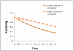
Table 2 Reliability w.r.t. time

Time (T)	Reliability (R)
0.0	1
0.5	[0.90021,0.97140]
1	[0.81018, 0.93817]
1.5	[0.72898,0.90156]
2	[0.65578,0.862639]
2.5	[0.589807,0.82226]
3	[0.53036,0.781161]
3.5	[0.476813,0.73990]
4	[0.428594,0.69895]
4.5	[0.385183,0.65869]
5	[0.346111,0.61940]

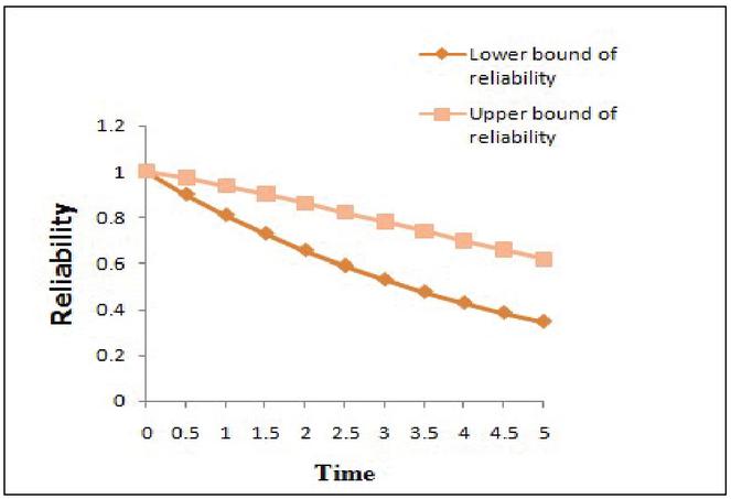
Figure 2 Reliability vs. time.

5 Mean Time to Failure of the Repairable Multi-state Parallel-series System

MTTF is a measurement of the average failure time and applicable to non-maintained units which are working under specified conditions. Generally, MTTF is evaluated from data taken over a period of time in which all the system units are not failed. In other words, the expectation of a random variable T is called MTTF.

Mathematically, MTTF is defined as

$$\text{MTTF}=\underset{s\to 0}{lim}R(s)$$

(43)

where R(s) is the Laplace transform of R(t).

By Equation (43), the MTTF of considered system can be evaluated as follows:

$\mathrm{MTTF}$	$=[{\displaystyle \frac{(\overline{{\lambda }_{21}}-\overline{{\lambda }_{32}})\overline{{\lambda }_{32}}+{\underset{¯}{{\lambda }_{32}}}^2}{3{\overline{{\lambda }_{32}}}^2(\overline{{\lambda }_{21}}-\overline{{\lambda }_{32}})}}-{\displaystyle \frac{\left(4\overline{{\lambda }_{32}}+\overline{{\lambda }_{21}}\right){\underset{¯}{{\lambda }_{32}}}^2}{2(\overline{{\lambda }_{21}}-\overline{{\lambda }_{32}})\overline{{\lambda }_{32}}{(2\overline{{\lambda }_{32}}+0.491\overline{{\lambda }_{21}})}^2}}$
	$\mathrm{\hspace{1em}}+{\displaystyle \frac{\left\{2\underset{¯}{{\lambda }_{32}}(\overline{{\lambda }_{21}}-\overline{{\lambda }_{32}})\overline{{\lambda }_{32}}-{\underset{¯}{{\lambda }_{32}}}^2(\overline{{\lambda }_{21}}-2\overline{{\lambda }_{32}})\right\}}{2(\overline{{\lambda }_{21}}-\overline{{\lambda }_{32}})\overline{{\lambda }_{32}}{(2\overline{{\lambda }_{32}}+0.491\overline{{\lambda }_{21}})}^2}}$
	$\mathrm{\hspace{1em}}\cdot {\displaystyle \frac{(\underset{¯}{{\lambda }_{21}}-\underset{¯}{{\lambda }_{32}})\underset{¯}{{\lambda }_{32}}+{\overline{{\lambda }_{32}}}^2}{3{\underset{¯}{{\lambda }_{32}}}^2(\underset{¯}{{\lambda }_{21}}-\underset{¯}{{\lambda }_{32}})}}-{\displaystyle \frac{(4\underset{¯}{{\lambda }_{32}}+\underset{¯}{{\lambda }_{21}}){\overline{{\lambda }_{32}}}^2}{2(\underset{¯}{{\lambda }_{21}}-\underset{¯}{{\lambda }_{32}})\underset{¯}{{\lambda }_{32}}{(2\underset{¯}{{\lambda }_{32}}+0.491\underset{¯}{{\lambda }_{21}})}^2}}$
	$\mathrm{\hspace{1em}}+{\displaystyle \frac{\left\{2\underset{¯}{{\lambda }_{32}}(\underset{¯}{{\lambda }_{21}}-\underset{¯}{{\lambda }_{32}})\overline{{\lambda }_{32}}-{\overline{{\lambda }_{32}}}^2(\underset{¯}{{\lambda }_{21}}-2\underset{¯}{{\lambda }_{32}})\right\}}{2(\underset{¯}{{\lambda }_{21}}-\underset{¯}{{\lambda }_{32}})\underset{¯}{{\lambda }_{32}}{(2\underset{¯}{{\lambda }_{32}}+0.491{\lambda }_{21})}^2}}]$	(44)

From Equation (44), one can get variations on MTTF of the repairable multi-state parallel-series system with respect to ${\underset{¯}{\lambda }}_{32},{\overline{\lambda }}_{32},{\underset{¯}{\lambda }}_{21}$ and ${\overline{\lambda }}_{21}$ as listed in the Tables 3 to 6, and the same are shown in the Figures 3 to 6 respectively.

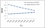
Table 3 MTTF w.r.t. ${\underset{¯}{\lambda }}_{32}$

${\underset{¯}{\lambda }}_{32}$	MTTF
0.09	[4.815692,6.529393]
0.091	[4.848816,6.398053]
0.092	[4.882306,6.2714]
0.093	[4.916163,6.149211]
0.094	[4.950385,6.031272]
0.095	[4.984973,5.917385]
0.096	[5.019928,5.807362]
0.097	[5.055248,5.701024]
0.098	[5.090934,5.598205]
0.099	[5.126987,5.498746]

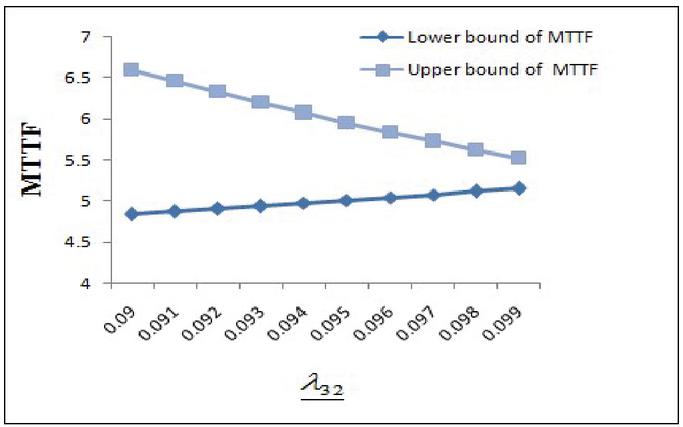
Figure 3 MTTF v/s ${\underset{¯}{\lambda }}_{32}$.

Table 4 MTTF w.r.t. ${\underset{¯}{\lambda }}_{32}$

${\underset{¯}{\lambda }}_{32}$	MTTF
0.1	[4.8156,6.5293]
0.2	[1.8419,13.1816]
0.3	[1.1623,23.4763]
0.4	[0.85479,37.4110]
0.5	[0.67761,54.9853]
0.6	[0.56187,76.199]
0.7	[0.48016,101.05]
0.8	[0.41932,129.544]
0.9	[0.37223,161.676]
0.91	[0.36810,165.089]

Figure 4 MTTF v/s ${\underset{¯}{\lambda }}_{32}$.

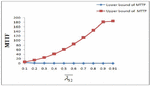
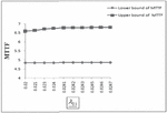
Table 5 MTTF w.r.t. ${\underset{¯}{\lambda }}_{21}$

${\underset{¯}{\lambda }}_{21}$	MTTF
0.02	[4.8156,6.5293]
0.021	[4.8156,6.5639]
0.023	[4.81569,6.6359]
0.024	[4.81569,6.6734]
0.0241	[4.81569,6.6772]
0.0242	[4.81569,6.6810]
0.0243	[4.81569,6.6849]
0.0245	[4.81569,6.6926]
0.0246	[4.81569,6.6965]
0.0247	[4.81569,6.7003]

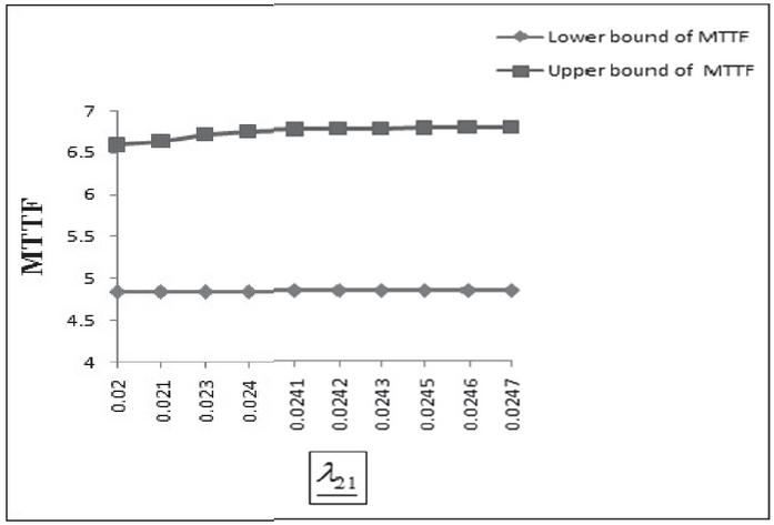
Figure 5 MTTF v/s ${\underset{¯}{\lambda }}_{21}$.

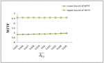
Table 6 MTTF w.r.t. ${\underset{¯}{\lambda }}_{21}$

${\underset{¯}{\lambda }}_{21}$	MTTF
0.025	[4.81569, 6.52939]
0.026	[4.82363, 6.52939]
0.027	[4.83184, 6.52939]
0.028	[4.8403, 6.529393]
0.029	[4.84914, 6.52939]
0.03	[4.85825, 6.52939]
0.031	[4.86769, 6.52939]
0.032	[4.8774, 6.529393]
0.034	[4.8980, 6.529393]
0.035	[4.90894, 6.52939]

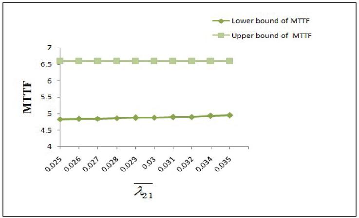
Figure 6 MTTF v/s ${\underset{¯}{\lambda }}_{21}$.

6 Sensitivity of the Repairable Multi-state Parallel-series System

Sensitivity analysis is a measure of the rate of change in the output of a system due to a change in the input of the system. It is like the Birnbaum importance. Parameters that affect modeling error, optimization of system and evaluation of reliability is possible with the help of sensitivity. Here, $R$ is the reliability and $\mu$ is parameter of the model of the system is given by the sensitivity S corresponding to $\mu$ is given by:

$$S=\frac{\partial R}{\partial \mu }$$

(45)

Using Equation (45) sensitivity of the considered model w.r.t. different parameters can be evaluated as:

(i) Lower bound sensitivity w.r.t. $\underset{¯}{{\lambda }_{32}}$is given by

$\underset{¯}{S_{\underset{¯}{{\lambda }_{32}}}}$	$={\displaystyle \frac{\partial \underset{¯}{R}}{\partial \underset{¯}{{\lambda }_{32}}}}={\displaystyle \frac{e^{-t\left(\frac{4\overline{{\lambda }_{32}}+\overline{{\mu }_{12}}+\overline{{\lambda }_{21}}}{2}\right)}\sinh \left(t\sqrt{\frac{{(\overline{{\mu }_{12}}-\overline{{\lambda }_{21}})}^2}{4}+\underset{¯}{{\lambda }_{21}}\underset{¯}{{\mu }_{12}}}\right)}{\sqrt{\frac{{(\overline{{\mu }_{12}}-\overline{{\lambda }_{21}})}^2}{4}+\underset{¯}{{\lambda }_{21}}\underset{¯}{{\mu }_{12}}}}}$
	$\mathrm{\hspace{1em}}+{\displaystyle \frac{e^{-t2\overline{{\lambda }_{32}}}(1-\overline{{\mu }_{12}})}{(\overline{{\mu }_{12}}+\overline{{\lambda }_{21}}-\overline{{\lambda }_{32}})\overline{{\lambda }_{32}}-\overline{{\lambda }_{21}}\overline{{\mu }_{12}}+\underset{¯}{{\lambda }_{21}}\underset{¯}{{\mu }_{12}}}}$
	$\mathrm{\hspace{1em}}\times [e^{-t\overline{{\lambda }_{32}}}-e^{-t\frac{\overline{{\mu }_{12}}+\overline{{\lambda }_{21}}}{2}}\{\cosh \left(t\sqrt{{\displaystyle \frac{{(\overline{{\mu }_{12}}-\overline{{\lambda }_{21}})}^2}{4}}+\underset{¯}{{\lambda }_{21}}\underset{¯}{{\mu }_{12}}}\right)$
	$\mathrm{\hspace{1em}}+\left({\displaystyle \frac{\overline{{\mu }_{12}}+\overline{{\lambda }_{21}}-2\overline{{\lambda }_{32}}}{2}}\right){\displaystyle \frac{\sinh \left(t\sqrt{\frac{{(\overline{{\mu }_{12}}-\overline{{\lambda }_{21}})}^2}{4}+\underset{¯}{{\lambda }_{21}}\underset{¯}{{\mu }_{12}}}\right)}{\sqrt{\frac{{(\overline{{\mu }_{12}}-\overline{{\lambda }_{21}})}^2}{4}+\underset{¯}{{\lambda }_{21}}\underset{¯}{{\mu }_{12}}}}}\}]$	(46)

(ii) Upper bound sensitivity w.r.t. ${\overline{\lambda }}_{32}$is obtained as

$\overline{S_{\overline{{\lambda }_{32}}}}$	$={\displaystyle \frac{\partial \overline{R}}{\partial \overline{{\lambda }_{32}}}}={\displaystyle \frac{e^{-t\left(\frac{4\underset{¯}{{\lambda }_{32}}+\underset{¯}{{\mu }_{12}}+\underset{¯}{{\lambda }_{21}}}{2}\right)}\sinh \left(t\sqrt{\frac{{(\underset{¯}{{\mu }_{12}}-\underset{¯}{{\lambda }_{21}})}^2}{4}+\overline{{\lambda }_{21}}\overline{{\mu }_{12}}}\right)}{\sqrt{\frac{{(\underset{¯}{{\mu }_{12}}-\underset{¯}{{\lambda }_{21}})}^2}{4}+\overline{{\lambda }_{21}}\overline{{\mu }_{12}}}}}$
	$\mathrm{\hspace{1em}}+{\displaystyle \frac{e^{-t2\underset{¯}{{\lambda }_{32}}}\left(1-\underset{¯}{{\mu }_{12}}\right)}{\left(\underset{¯}{{\mu }_{12}}+\underset{¯}{{\lambda }_{21}}-\underset{¯}{{\lambda }_{32}}\right)\underset{¯}{{\lambda }_{32}}+\overline{{\lambda }_{21}}\overline{{\mu }_{12}}-\underset{¯}{{\lambda }_{21}}\underset{¯}{{\mu }_{12}}}}$
	$\mathrm{\hspace{1em}}\times [e^{-t\underset{¯}{{\lambda }_{32}}}-e^{-t\frac{\underset{¯}{{\mu }_{12}}+\underset{¯}{{\lambda }_{21}}}{2}}\{\cosh \left(t\sqrt{{\displaystyle \frac{{(\underset{¯}{{\mu }_{12}}-\underset{¯}{{\lambda }_{21}})}^2}{4}}+\overline{{\lambda }_{21}}\overline{{\mu }_{12}}}\right)$
	$\mathrm{\hspace{1em}}+\left({\displaystyle \frac{\underset{¯}{{\mu }_{12}}+\underset{¯}{{\lambda }_{21}}-2\underset{¯}{{\lambda }_{32}}}{2}}\right){\displaystyle \frac{\sinh \left(t\sqrt{\frac{{(\underset{¯}{{\mu }_{12}}-\underset{¯}{{\lambda }_{21}})}^2}{4}+\overline{{\lambda }_{21}}\overline{{\mu }_{12}}}\right)}{\sqrt{\frac{{(\underset{¯}{{\mu }_{12}}-\underset{¯}{{\lambda }_{21}})}^2}{4}+\overline{{\lambda }_{21}}\overline{{\mu }_{12}}}}}\}]$	(47)

(iii) Lower bound sensitivity w.r.t. $\overline{{\lambda }_{32}}$ is evaluated as:

$\underset{¯}{S_{\overline{{\lambda }_{32}}}}$	$={\displaystyle \frac{\partial \underset{¯}{R}}{\partial \overline{{\lambda }_{32}}}}$
	$=-3t{e}^{-3\overline{{\lambda }_{32}}t}-{\displaystyle \frac{2t\underset{¯}{{\lambda }_{32}}(\underset{¯}{{\lambda }_{32}}-\overline{{\mu }_{12}})e^{-2\overline{{\lambda }_{32}}t}}{(\overline{{\mu }_{12}}+\overline{{\lambda }_{21}}-\overline{{\lambda }_{32}})\overline{{\lambda }_{32}}-\overline{{\lambda }_{21}}\overline{{\mu }_{12}}+\underset{¯}{{\lambda }_{21}}\underset{¯}{{\mu }_{12}}}}$
	$\mathrm{\hspace{1em}}[e^{-t\overline{{\lambda }_{32}}}+e^{-\frac{\overline{({\mu }_{12}}+\overline{{\lambda }_{21})}}{2}t}$
	$\mathrm{\hspace{1em}}\times \{{\displaystyle \frac{\left(\overline{{\mu }_{12}}+\overline{{\lambda }_{21}}\right)\sinh \left(t\sqrt{\frac{{(\overline{{\mu }_{12}}-\overline{{\lambda }_{21}})}^2}{4}+\underset{¯}{{\lambda }_{21}}\underset{¯}{{\mu }_{12}}}\right)}{2\sqrt{\frac{{(\overline{{\mu }_{12}}-\overline{{\lambda }_{21}})}^2}{4}+\underset{¯}{{\lambda }_{21}}\underset{¯}{{\mu }_{12}}}}}$
	$\mathrm{\hspace{1em}}-\cosh \left(t\sqrt{{\displaystyle \frac{{(\overline{{\mu }_{12}}-\overline{{\lambda }_{21}})}^2}{4}}+\underset{¯}{{\lambda }_{21}}\underset{¯}{{\mu }_{12}}}\right)\}]$
	$\mathrm{\hspace{1em}}-{\displaystyle \frac{2t{e}^{-t\frac{\overline{{\mu }_{12}}+\overline{{\lambda }_{21}}+4\overline{{\lambda }_{32}}}{2}}\sinh \left(t\sqrt{\frac{{(\overline{{\mu }_{12}}-\overline{{\lambda }_{21}})}^2}{4}+\underset{¯}{{\lambda }_{21}}\underset{¯}{{\mu }_{12}}}\right)}{\sqrt{\frac{{(\overline{{\mu }_{12}}-\overline{{\lambda }_{21}})}^2}{4}+\underset{¯}{{\lambda }_{21}}\underset{¯}{{\mu }_{12}}}}}$
	$\mathrm{\hspace{1em}}\times \left\{\underset{¯}{{\lambda }_{32}}-{\displaystyle \frac{\underset{¯}{{\lambda }_{32}}\left(\underset{¯}{{\lambda }_{32}}-\overline{{\mu }_{12}}\right)(\overline{{\mu }_{12}}+\overline{{\lambda }_{21}}-\overline{{\lambda }_{32}})}{(\overline{{\mu }_{12}}+\overline{{\lambda }_{21}}-\overline{{\lambda }_{32}})\overline{{\lambda }_{32}}-\overline{{\lambda }_{21}}\overline{{\mu }_{12}}+\underset{¯}{{\lambda }_{21}}\underset{¯}{{\mu }_{12}}}}\right\}$
	$\mathrm{\hspace{1em}}+{\displaystyle \frac{\underset{¯}{{\lambda }_{32}}\left(1-\overline{{\mu }_{12}}\right)\left(\overline{{\mu }_{12}}+\overline{{\lambda }_{21}}-2\overline{{\lambda }_{32}}\right)e^{-t\frac{\overline{{\mu }_{12}}+\overline{{\lambda }_{21}}+2\overline{{\lambda }_{32}}}{2}}}{{\left((\overline{{\mu }_{12}}+\overline{{\lambda }_{21}}-\overline{{\lambda }_{32}})\overline{{\lambda }_{32}}-\overline{{\lambda }_{21}}\overline{{\mu }_{12}}+\underset{¯}{{\lambda }_{21}}\underset{¯}{{\mu }_{12}}\right)}^2}}$
	$\mathrm{\hspace{1em}}\{\cosh \left(t\sqrt{{\displaystyle \frac{{(\overline{{\mu }_{12}}-\overline{{\lambda }_{21}})}^2}{4}}+\underset{¯}{{\lambda }_{21}}\underset{¯}{{\mu }_{12}}}\right)$
	$\mathrm{\hspace{1em}}-{\displaystyle \frac{\left(2\overline{{\lambda }_{32}}-\overline{{\mu }_{12}}-\overline{{\lambda }_{21}}\right)\sinh \left(t\sqrt{\frac{{(\overline{{\mu }_{12}}-\overline{{\lambda }_{21}})}^2}{4}+\underset{¯}{{\lambda }_{21}}\underset{¯}{{\mu }_{12}}}\right)}{2\sqrt{\frac{{(\overline{{\mu }_{12}}-\overline{{\lambda }_{21}})}^2}{4}+\underset{¯}{{\lambda }_{21}}\underset{¯}{{\mu }_{12}}}}}$	(48)

(iv) Upper bound sensitivity w.r.t. ${\overline{\lambda }}_{32}$ is given by

$\overline{S_{\underset{¯}{{\lambda }_{32}}}}$	$={\displaystyle \frac{\partial \overline{R}}{\partial \underset{¯}{{\lambda }_{32}}}}=-3t{e}^{-3\underset{¯}{{\lambda }_{32}}t}-{\displaystyle \frac{2t\overline{{\lambda }_{32}}(\overline{{\lambda }_{32}}-\overline{{\mu }_{12}})e^{-2\underset{¯}{{\lambda }_{32}}t}}{(\underset{¯}{{\mu }_{12}}+\underset{¯}{{\lambda }_{21}}-\underset{¯}{{\lambda }_{32}})\underset{¯}{{\lambda }_{32}}+\overline{{\lambda }_{21}}\overline{{\mu }_{12}}-\underset{¯}{{\lambda }_{21}}\underset{¯}{{\mu }_{12}}}}$
	$\mathrm{\hspace{1em}}[e^{-t\underset{¯}{{\lambda }_{32}}}+e^{-\frac{(\underset{¯}{{\mu }_{12}}+\underset{¯}{{\lambda }_{21}})}{2}t}$
	$\mathrm{\hspace{1em}}\times \{{\displaystyle \frac{\left(\underset{¯}{{\mu }_{12}}+\underset{¯}{{\lambda }_{21}}\right)\sinh \left(t\sqrt{\frac{{(\underset{¯}{{\mu }_{12}}-\underset{¯}{{\lambda }_{21}})}^2}{4}+\overline{{\lambda }_{21}}\overline{{\mu }_{12}}}\right)}{2\sqrt{\frac{{(\underset{¯}{{\mu }_{12}}-\underset{¯}{{\lambda }_{21}})}^2}{4}+\overline{{\lambda }_{21}}\overline{{\mu }_{12}}}}}$
	$\mathrm{\hspace{1em}}-\cosh \left(t\sqrt{{\displaystyle \frac{{(\underset{¯}{{\mu }_{12}}-\underset{¯}{{\lambda }_{21}})}^2}{4}}+\overline{{\lambda }_{21}}\overline{{\mu }_{12}}}\right)\}]$
	$\mathrm{\hspace{1em}}-{\displaystyle \frac{2t{e}^{-t\frac{\underset{¯}{{\mu }_{12}}+\underset{¯}{{\lambda }_{21}}+4\underset{¯}{{\lambda }_{32}}}{2}}\sinh \left(t\sqrt{\frac{{(\underset{¯}{{\mu }_{12}}-\underset{¯}{{\lambda }_{21}})}^2}{4}+\overline{{\lambda }_{21}}\overline{{\mu }_{12}}}\right)}{\sqrt{\frac{{(\underset{¯}{{\mu }_{12}}-\underset{¯}{{\lambda }_{21}})}^2}{4}+\overline{{\lambda }_{21}}\overline{{\mu }_{12}}}}}$
	$\mathrm{\hspace{1em}}\left[\overline{{\lambda }_{32}}-{\displaystyle \frac{\overline{{\lambda }_{32}}\left(\overline{{\lambda }_{32}}-\underset{¯}{{\mu }_{12}}\right)(\underset{¯}{{\mu }_{12}}+\underset{¯}{{\lambda }_{21}}-\underset{¯}{{\lambda }_{32}})}{(\underset{¯}{{\mu }_{12}}+\underset{¯}{{\lambda }_{21}}-\underset{¯}{{\lambda }_{32}})\underset{¯}{{\lambda }_{32}}+\overline{{\lambda }_{21}}\overline{{\mu }_{12}}-\underset{¯}{{\lambda }_{21}}\underset{¯}{{\mu }_{12}}}}\right]$
	$\mathrm{\hspace{1em}}+\cosh \left(t\sqrt{{\displaystyle \frac{{(\underset{¯}{{\mu }_{12}}-\underset{¯}{{\lambda }_{21}})}^2}{4}}+\overline{{\lambda }_{21}}\overline{{\mu }_{12}}}\right)$
	$\mathrm{\hspace{1em}}\left\{+{\displaystyle \frac{\left((\underset{¯}{{\mu }_{12}}+\underset{¯}{{\lambda }_{21}}-2\underset{¯}{{\lambda }_{32}})\right)\sinh \left(t\sqrt{\frac{{(\underset{¯}{{\mu }_{12}}-\underset{¯}{{\lambda }_{21}})}^2}{4}+\overline{{\lambda }_{21}}\overline{{\mu }_{12}}}\right)}{2\sqrt{\frac{{(\underset{¯}{{\mu }_{12}}-\underset{¯}{{\lambda }_{21}})}^2}{4}+\overline{{\lambda }_{21}}\overline{{\mu }_{12}}}}}\right\}$
	$\mathrm{\hspace{1em}}\times {\displaystyle \frac{\overline{{\lambda }_{32}}\left(1-\underset{¯}{{\mu }_{12}}\right)(\underset{¯}{{\mu }_{12}}+\underset{¯}{{\lambda }_{21}}-\underset{¯}{2{\lambda }_{32}})e^{-t\frac{\underset{¯}{{\mu }_{12}}+\underset{¯}{{\lambda }_{21}}+2\underset{¯}{{\lambda }_{32}}}{2}}}{{\left\{(\underset{¯}{{\mu }_{12}}+\underset{¯}{{\lambda }_{21}}-\underset{¯}{{\lambda }_{32}})\underset{¯}{{\lambda }_{32}}+\overline{{\lambda }_{21}}\overline{{\mu }_{12}}-\underset{¯}{{\lambda }_{21}}\underset{¯}{{\mu }_{12}}\right\}}^2}}$	(49)

(v) Lower bound sensitivity w.r.t. ${\underset{¯}{\lambda }}_{21}$ is computed as

$\underset{¯}{S_{\underset{¯}{{\lambda }_{21}}}}$	$={\displaystyle \frac{\partial \underset{¯}{R}}{\partial \underset{¯}{{\lambda }_{21}}}}=e^{-t\frac{\overline{{\mu }_{12}}+\overline{{\lambda }_{21}}+4\overline{{\lambda }_{32}}}{2}}$
	$\mathrm{\hspace{1em}}[{\displaystyle \frac{\underset{¯}{{\mu }_{12}}\underset{¯}{{\lambda }_{32}}\left(\underset{¯}{{\lambda }_{32}}-\overline{{\mu }_{12}}\right)}{{\left((\overline{{\mu }_{12}}+\overline{{\lambda }_{21}}-\overline{{\lambda }_{32}})\overline{{\lambda }_{32}}-\overline{{\lambda }_{21}}\overline{{\mu }_{12}}+\underset{¯}{{\lambda }_{21}}\underset{¯}{{\mu }_{12}}\right)}^2}}$
	$\mathrm{\hspace{1em}}\{\cosh \left({\displaystyle \frac{t}{2}}\sqrt{{(\overline{{\mu }_{12}}-\overline{{\lambda }_{21}})}^2+4\underset{¯}{{\lambda }_{21}}\underset{¯}{{\mu }_{12}}}\right)$
	$\mathrm{\hspace{1em}}-{\displaystyle \frac{\left(2\overline{{\lambda }_{32}}-\overline{{\mu }_{12}}-\overline{{\lambda }_{21}}\right)\sinh \left(\frac{t}{2}\sqrt{{(\overline{{\mu }_{12}}-\overline{{\lambda }_{21}})}^2+4\underset{¯}{{\lambda }_{21}}\underset{¯}{{\mu }_{12}}}\right)}{\sqrt{{(\overline{{\mu }_{12}}-\overline{{\lambda }_{21}})}^2+4\underset{¯}{{\lambda }_{21}}\underset{¯}{{\mu }_{12}}}}}\}$
	$\mathrm{\hspace{1em}}+{\displaystyle \frac{\underset{¯}{{\mu }_{12}}}{\sqrt{{(\overline{{\mu }_{12}}-\overline{{\lambda }_{21}})}^2+4\underset{¯}{{\lambda }_{21}}\underset{¯}{{\mu }_{12}}}}}$
	$\mathrm{\hspace{1em}}\{{\displaystyle \frac{-t\underset{¯}{{\lambda }_{32}}\left(\underset{¯}{{\lambda }_{32}}-\overline{{\mu }_{12}}\right)\sinh \left(\frac{t}{2}\sqrt{{(\overline{{\mu }_{12}}-\overline{{\lambda }_{21}})}^2+4\underset{¯}{{\lambda }_{21}}\underset{¯}{{\mu }_{12}}}\right)}{(\overline{{\mu }_{12}}+\overline{{\lambda }_{21}}-\overline{{\lambda }_{32}})\overline{{\lambda }_{32}}-\overline{{\lambda }_{21}}\overline{{\mu }_{12}}+\underset{¯}{{\lambda }_{21}}\underset{¯}{{\mu }_{12}}}}$
	$\mathrm{\hspace{1em}}-{\displaystyle \frac{\begin{array}{c}2\underset{¯}{{\lambda }_{32}}[2\{\overline{{\lambda }_{21}}\overline{{\lambda }_{32}}-{\overline{{\lambda }_{32}}}^2+\underset{¯}{{\lambda }_{21}}\underset{¯}{{\mu }_{12}}\}\hfill \\ +\{\underset{¯}{{\lambda }_{32}}(\overline{{\mu }_{12}}-\overline{{\lambda }_{21}})+{\overline{{\mu }_{12}}}^2-\overline{{\lambda }_{21}}\overline{{\mu }_{12}}\}]\hfill \end{array}}{\begin{array}{c}\{(\overline{{\mu }_{12}}+\overline{{\lambda }_{21}}-\overline{{\lambda }_{32}})\overline{{\lambda }_{32}}-\overline{{\lambda }_{21}}\overline{{\mu }_{12}}+\underset{¯}{{\lambda }_{21}}\underset{¯}{{\mu }_{12}}\}\hfill \\ \{{(\overline{{\mu }_{12}}-\overline{{\lambda }_{21}})}^2+4\underset{¯}{{\lambda }_{21}}\underset{¯}{{\mu }_{12}}\}\hfill \end{array}}}$
	$\mathrm{\hspace{1em}}\times \{\sinh \left({\displaystyle \frac{t}{2}}\sqrt{{(\overline{{\mu }_{12}}-\overline{{\lambda }_{21}})}^2+4\underset{¯}{{\lambda }_{21}}\underset{¯}{{\mu }_{12}}}\right)$
	$\mathrm{\hspace{1em}}-{\displaystyle \frac{t}{2}}\sqrt{{(\overline{{\mu }_{12}}-\overline{{\lambda }_{21}})}^2+4\underset{¯}{{\lambda }_{21}}\underset{¯}{{\mu }_{12}}}\cosh$
	$\mathrm{\hspace{1em}}\left({\displaystyle \frac{t}{2}}\sqrt{{(\overline{{\mu }_{12}}-\overline{{\lambda }_{21}})}^2+4\underset{¯}{{\lambda }_{21}}\underset{¯}{{\mu }_{12}}}\right)\}\}]$	(50)

(vi) Upper bound sensitivity w.r.t. ${\overline{\lambda }}_{21}$ is evaluated as:

$\overline{S_{\overline{{\lambda }_{21}}}}$	$={\displaystyle \frac{\partial \overline{R}}{\partial \overline{{\lambda }_{21}}}}$
	$=[{\displaystyle \frac{\overline{{\mu }_{12}}\overline{{\lambda }_{32}}\left(\overline{{\lambda }_{32}}-\underset{¯}{{\mu }_{12}}\right)}{{\left((\underset{¯}{{\mu }_{12}}+\underset{¯}{{\lambda }_{21}}-\underset{¯}{{\lambda }_{32}})\underset{¯}{{\lambda }_{32}}+\overline{{\lambda }_{21}}\overline{{\mu }_{12}}-\underset{¯}{{\lambda }_{21}}\underset{¯}{{\mu }_{12}}\right)}^2}}$
	$\mathrm{\hspace{1em}}\{\cosh \left({\displaystyle \frac{t}{2}}\sqrt{{(\underset{¯}{{\mu }_{12}}-\underset{¯}{{\lambda }_{21}})}^2+4\overline{{\lambda }_{21}}\overline{{\mu }_{12}}}\right)$
	$\mathrm{\hspace{1em}}-{\displaystyle \frac{\left(2\underset{¯}{{\lambda }_{32}}-\underset{¯}{{\mu }_{12}}-\underset{¯}{{\lambda }_{21}}\right)\sinh \left(\frac{t}{2}\sqrt{{(\underset{¯}{{\mu }_{12}}-\underset{¯}{{\lambda }_{21}})}^2+4\overline{{\lambda }_{21}}\overline{{\mu }_{12}}}\right)}{\sqrt{{(\underset{¯}{{\mu }_{12}}-\underset{¯}{{\lambda }_{21}})}^2+4\overline{{\lambda }_{21}}\overline{{\mu }_{12}}}}}\}$
	$\mathrm{\hspace{1em}}+{\displaystyle \frac{\overline{{\mu }_{12}}}{\sqrt{{(\underset{¯}{{\mu }_{12}}-\underset{¯}{{\lambda }_{21}})}^2+4\overline{{\lambda }_{21}}\overline{{\mu }_{12}}}}}$
	$\mathrm{\hspace{1em}}\times \{{\displaystyle \frac{-t\overline{{\lambda }_{32}}\left(\overline{{\lambda }_{32}}-\underset{¯}{{\mu }_{12}}\right)\sinh \left(\frac{t}{2}\sqrt{{(\underset{¯}{{\mu }_{12}}-\underset{¯}{{\lambda }_{21}})}^2+4\overline{{\lambda }_{21}}\overline{{\mu }_{12}}}\right)}{(\underset{¯}{{\mu }_{12}}+\underset{¯}{{\lambda }_{21}}-\underset{¯}{{\lambda }_{32}})\underset{¯}{{\lambda }_{32}}+\overline{{\lambda }_{21}}\overline{{\mu }_{12}}-\underset{¯}{{\lambda }_{21}}\underset{¯}{{\mu }_{12}}}}$
	$\mathrm{\hspace{1em}}-{\displaystyle \frac{\begin{array}{c}2\overline{{\lambda }_{32}}[2\{\underset{¯}{{\lambda }_{21}}{\lambda }_{32}-{\underset{¯}{{\lambda }_{32}}}^2+\overline{{\lambda }_{21}}\overline{{\mu }_{12}}\}\hfill \\ +\{\overline{{\lambda }_{32}}(\underset{¯}{{\mu }_{12}}-\underset{¯}{{\lambda }_{21}})+{\underset{¯}{{\mu }_{12}}}^2-\underset{¯}{{\lambda }_{21}}\underset{¯}{{\mu }_{12}}\}]\hfill \end{array}}{\begin{array}{c}\{(\underset{¯}{{\mu }_{12}}+\underset{¯}{{\lambda }_{21}}-\underset{¯}{{\lambda }_{32}})\underset{¯}{{\lambda }_{32}}+\overline{{\lambda }_{21}}\overline{{\mu }_{12}}-\underset{¯}{{\lambda }_{21}}\underset{¯}{{\mu }_{12}}\}\hfill \\ \{{(\underset{¯}{{\mu }_{12}}-\underset{¯}{{\lambda }_{21}})}^2+4\overline{{\lambda }_{21}}\overline{{\mu }_{12}}\}\hfill \end{array}}}$
	$\times \{\sinh \left({\displaystyle \frac{t}{2}}\sqrt{{(\underset{¯}{{\mu }_{12}}-\underset{¯}{{\lambda }_{21}})}^2+4\overline{{\lambda }_{21}}\overline{{\mu }_{12}}}\right)$
	$\mathrm{\hspace{1em}}-{\displaystyle \frac{t}{2}}\sqrt{{(\underset{¯}{{\mu }_{12}}-\underset{¯}{{\lambda }_{21}})}^2+4\overline{{\lambda }_{21}}\overline{{\mu }_{12}}}\cosh$
	$\mathrm{\hspace{1em}}\left({\displaystyle \frac{t}{2}}\sqrt{{(\underset{¯}{{\mu }_{12}}-\underset{¯}{{\lambda }_{21}})}^2+4\overline{{\lambda }_{21}}\overline{{\mu }_{12}}}\right)\}\}]$	(51)

(vii) Upper bound sensitivity w.r.t. ${\overline{\lambda }}_{21}$:

$\underset{¯}{S_{\overline{{\lambda }_{21}}}}$	$={\displaystyle \frac{\partial \underset{¯}{R}}{\partial \overline{{\lambda }_{21}}}}$
	$=e^{-2t\overline{{\lambda }_{32}}}[{\displaystyle \frac{\underset{¯}{{\lambda }_{32}}\left(\underset{¯}{{\lambda }_{32}}-\overline{{\mu }_{12}}\right)}{(\overline{{\mu }_{12}}+\overline{{\lambda }_{21}}-\overline{{\lambda }_{32}})\overline{{\lambda }_{32}}-\overline{{\lambda }_{21}}\overline{{\mu }_{12}}+\underset{¯}{{\lambda }_{21}}\underset{¯}{{\mu }_{12}}}}$
	$\mathrm{\hspace{1em}}\times \{{\displaystyle \frac{t}{2}}\cosh \left({\displaystyle \frac{t}{2}}\sqrt{{(\overline{{\mu }_{12}}-\overline{{\lambda }_{21}})}^2+4\underset{¯}{{\lambda }_{21}}\underset{¯}{{\mu }_{12}}}\right)$
	$\mathrm{\hspace{1em}}\left\{{\displaystyle \frac{\left(2\overline{{\lambda }_{32}}-\overline{{\mu }_{12}}-\overline{{\lambda }_{21}}\right)\left(\overline{{\lambda }_{21}}-\overline{{\mu }_{12}}\right)}{2\left\{{(\overline{{\mu }_{12}}-\overline{{\lambda }_{21}})}^2+4\underset{¯}{{\lambda }_{21}}\underset{¯}{{\mu }_{12}}\right\}}}{\displaystyle \frac{-e^{\frac{-t\left(\overline{{\mu }_{12}}+\overline{{\lambda }_{21}}\right)}{2}}}{2}}\right\}$
	$\mathrm{\hspace{1em}}-{\displaystyle \frac{\frac{\left(2\overline{{\lambda }_{32}}-\overline{{\mu }_{12}}-\overline{{\lambda }_{21}}\right)\left(\overline{{\lambda }_{21}}-\overline{{\mu }_{12}}\right)}{\left\{{(\overline{{\mu }_{12}}-\overline{{\lambda }_{21}})}^2+4\underset{¯}{{\lambda }_{21}}\underset{¯}{{\mu }_{12}}\right\}}+t{e}^{\frac{-t\left(\overline{{\mu }_{12}}+\overline{{\lambda }_{21}}\right)}{2}}\left(\overline{{\lambda }_{21}}-\overline{{\mu }_{12}}\right)+1}{2\sqrt{{(\overline{{\mu }_{12}}-\overline{{\lambda }_{21}})}^2+4\underset{¯}{{\lambda }_{21}}\underset{¯}{{\mu }_{12}}}}}$
	$\mathrm{\hspace{1em}}\times {\displaystyle \frac{\sinh \left(\frac{t}{2}\sqrt{{(\overline{{\mu }_{12}}-\overline{{\lambda }_{21}})}^2+4\underset{¯}{{\lambda }_{21}}\underset{¯}{{\mu }_{12}}}\right)}{2\sqrt{{(\overline{{\mu }_{12}}-\overline{{\lambda }_{21}})}^2+4\underset{¯}{{\lambda }_{21}}\underset{¯}{{\mu }_{12}}}}}\}$
	$\mathrm{\hspace{1em}}\times \{e^{-t\overline{{\lambda }_{32}}}-e^{\frac{-t\left(\overline{{\mu }_{12}}+\overline{{\lambda }_{21}}\right)}{2}}\cosh \left({\displaystyle \frac{t}{2}}\sqrt{{(\overline{{\mu }_{12}}-\overline{{\lambda }_{21}})}^2+4\underset{¯}{{\lambda }_{21}}\underset{¯}{{\mu }_{12}}}\right)$
	$\mathrm{\hspace{1em}}+{\displaystyle \frac{\left(2\overline{{\lambda }_{32}}-\overline{{\mu }_{12}}-\overline{{\lambda }_{21}}\right)\sinh \left(\frac{t}{2}\sqrt{{(\overline{{\mu }_{12}}-\overline{{\lambda }_{21}})}^2+4\underset{¯}{{\lambda }_{21}}\underset{¯}{{\mu }_{12}}}\right)}{2\sqrt{{(\overline{{\mu }_{12}}-\overline{{\lambda }_{21}})}^2+4\underset{¯}{{\lambda }_{21}}\underset{¯}{{\mu }_{12}}}}}\}$
	$\mathrm{\hspace{1em}}+\overline{{\lambda }_{32}}\{{\displaystyle \frac{(\overline{{\mu }_{12}}-\overline{{\lambda }_{21}})\sinh \left(\frac{t}{2}\sqrt{{(\overline{{\mu }_{12}}-\overline{{\lambda }_{21}})}^2+4\underset{¯}{{\lambda }_{21}}\underset{¯}{{\mu }_{12}}}\right)}{\sqrt{{(\overline{{\mu }_{12}}-\overline{{\lambda }_{21}})}^2+4\underset{¯}{{\lambda }_{21}}\underset{¯}{{\mu }_{12}}}}}$
	$\mathrm{\hspace{1em}}+{\displaystyle \frac{t\left(\overline{{\lambda }_{21}}-\overline{{\mu }_{12}}\right)}{2}}\cosh \left({\displaystyle \frac{t}{2}}\sqrt{{(\overline{{\mu }_{12}}-\overline{{\lambda }_{21}})}^2+4\underset{¯}{{\lambda }_{21}}\underset{¯}{{\mu }_{12}}}\right)\}]$	(52)

(viii) Lower bound sensitivity w.r.t. $\underset{¯}{{\lambda }_{21}}$:

$\overline{S_{\underset{¯}{{\lambda }_{21}}}}$	$={\displaystyle \frac{\partial \overline{R}}{\partial \underset{¯}{{\lambda }_{21}}}}$
	$=e^{-2t\underset{¯}{{\lambda }_{32}}}[{\displaystyle \frac{\overline{{\lambda }_{32}}\left(\overline{{\lambda }_{32}}-\underset{¯}{{\mu }_{12}}\right)}{(\underset{¯}{{\mu }_{12}}+\underset{¯}{{\lambda }_{21}}-\underset{¯}{{\lambda }_{32}})\underset{¯}{{\lambda }_{32}}+\overline{{\lambda }_{21}}\overline{{\mu }_{12}}-\underset{¯}{{\lambda }_{21}}\underset{¯}{{\mu }_{12}}}}$
	$\mathrm{\hspace{1em}}\times \{t\cosh \left({\displaystyle \frac{t}{2}}\sqrt{{(\underset{¯}{{\mu }_{12}}-\underset{¯}{{\lambda }_{21}})}^2+4\overline{{\lambda }_{21}}\overline{{\mu }_{12}}}\right)$
	$\mathrm{\hspace{1em}}\left\{{\displaystyle \frac{\left(2\underset{¯}{{\lambda }_{32}}-\underset{¯}{{\mu }_{12}}-\underset{¯}{{\lambda }_{21}}\right)\left(\underset{¯}{{\lambda }_{21}}-\underset{¯}{{\mu }_{12}}\right)}{4\left\{{(\underset{¯}{{\mu }_{12}}-\underset{¯}{{\lambda }_{21}})}^2+4\overline{{\lambda }_{21}}\overline{{\mu }_{12}}\right\}}}{\displaystyle \frac{-e^{\frac{-t\left(\underset{¯}{{\mu }_{12}}+\underset{¯}{{\lambda }_{21}}\right)}{2}}}{2}}\right\}$
	$\mathrm{\hspace{1em}}{\displaystyle \frac{-\sinh \left(\frac{t}{2}\sqrt{{(\underset{¯}{{\mu }_{12}}-\underset{¯}{{\lambda }_{21}})}^2+4\overline{{\lambda }_{21}}\overline{{\mu }_{12}}}\right)}{2\sqrt{{(\underset{¯}{{\mu }_{12}}-\underset{¯}{{\lambda }_{21}})}^2+4\overline{{\lambda }_{21}}\overline{{\mu }_{12}}}}}$
	$\mathrm{\hspace{1em}}\times {\displaystyle \frac{\left\{\frac{\left(2\underset{¯}{{\lambda }_{32}}-\underset{¯}{{\mu }_{12}}-\underset{¯}{{\lambda }_{21}}\right)\left(\underset{¯}{{\lambda }_{21}}-\underset{¯}{{\mu }_{12}}\right)}{{(\underset{¯}{{\mu }_{12}}-\underset{¯}{{\lambda }_{21}})}^2+4\overline{{\lambda }_{21}}\overline{{\mu }_{12}}}+t{e}^{\frac{-t\left(\underset{¯}{{\mu }_{12}}+\underset{¯}{{\lambda }_{21}}\right)}{2}}\left(\underset{¯}{{\lambda }_{21}}-\underset{¯}{{\mu }_{12}}\right)+1\right\}}{2\sqrt{{(\underset{¯}{{\mu }_{12}}-\underset{¯}{{\lambda }_{21}})}^2+4\overline{{\lambda }_{21}}\overline{{\mu }_{12}}}}}$
	$\mathrm{\hspace{1em}}-{\displaystyle \frac{\overline{{\lambda }_{32}}{\left(\overline{{\lambda }_{32}}-\underset{¯}{{\mu }_{12}}\right)}^2}{{\left\{(\underset{¯}{{\mu }_{12}}+\underset{¯}{{\lambda }_{21}}-\underset{¯}{{\lambda }_{32}})\underset{¯}{{\lambda }_{32}}+\overline{{\lambda }_{21}}\overline{{\mu }_{12}}-\underset{¯}{{\lambda }_{21}}\underset{¯}{{\mu }_{12}}\right\}}^2}}$
	$\mathrm{\hspace{1em}}\times \{e^{-t\underset{¯}{{\lambda }_{32}}}-e^{\frac{-t\left(\underset{¯}{{\mu }_{12}}+\underset{¯}{{\lambda }_{21}}\right)}{2}}\cosh \left({\displaystyle \frac{t}{2}}\sqrt{{(\underset{¯}{{\mu }_{12}}-\underset{¯}{{\lambda }_{21}})}^2+4\overline{{\lambda }_{21}}\overline{{\mu }_{12}}}\right)$
	$\mathrm{\hspace{1em}}+{\displaystyle \frac{\left(2\underset{¯}{{\lambda }_{32}}-\underset{¯}{{\mu }_{12}}-\underset{¯}{{\lambda }_{21}}\right)\sinh \left(\frac{t}{2}\sqrt{{(\underset{¯}{{\mu }_{12}}-\underset{¯}{{\lambda }_{21}})}^2+4\overline{{\lambda }_{21}}\overline{{\mu }_{12}}}\right)}{2\sqrt{{(\underset{¯}{{\mu }_{12}}-\underset{¯}{{\lambda }_{21}})}^2+4\overline{{\lambda }_{21}}\overline{{\mu }_{12}}}}}\}$
	$\mathrm{\hspace{1em}}+\underset{¯}{{\lambda }_{32}}\{{\displaystyle \frac{(\underset{¯}{{\mu }_{12}}-\underset{¯}{{\lambda }_{21}})\sinh \left(\frac{t}{2}\sqrt{{(\underset{¯}{{\mu }_{12}}-\underset{¯}{{\lambda }_{21}})}^2+4\overline{{\lambda }_{21}}\overline{{\mu }_{12}}}\right)}{\sqrt{{(\underset{¯}{{\mu }_{12}}-\underset{¯}{{\lambda }_{21}})}^2+4\overline{{\lambda }_{21}}\overline{{\mu }_{12}}}}}$
	$\mathrm{\hspace{1em}}+{\displaystyle \frac{t\left(\underset{¯}{{\lambda }_{21}}-\underset{¯}{{\mu }_{12}}\right)}{2}}\cosh \left({\displaystyle \frac{t}{2}}\sqrt{{(\underset{¯}{{\mu }_{12}}-\underset{¯}{{\lambda }_{21}})}^2+4\overline{{\lambda }_{21}}\overline{{\mu }_{12}}}\right)\}]$	(53)

(ix) Lower bound sensitivity w.r.t. $\underset{¯}{{\mu }_{12}}$:

$\underset{¯}{S_{\underset{¯}{{\mu }_{12}}}}$	$={\displaystyle \frac{\partial \underset{¯}{R}}{\partial \underset{¯}{{\mu }_{12}}}}=e^{-2t\overline{{\lambda }_{32}}}[{\displaystyle \frac{\underset{¯}{{\lambda }_{32}}\left(\underset{¯}{{\lambda }_{32}}-\overline{{\mu }_{12}}\right)}{(\overline{{\mu }_{12}}+\overline{{\lambda }_{21}}-\overline{{\lambda }_{32}})\overline{{\lambda }_{32}}-\overline{{\lambda }_{21}}\overline{{\mu }_{12}}+\underset{¯}{{\lambda }_{21}}\underset{¯}{{\mu }_{12}}}}$
	$\mathrm{\hspace{1em}}\times \{{\displaystyle \frac{-e^{\frac{-t\left(\overline{{\mu }_{12}}+\overline{{\lambda }_{21}}\right)}{2}}t\underset{¯}{{\lambda }_{21}}\sinh \left(\frac{t}{2}\sqrt{{(\overline{{\mu }_{12}}-\overline{{\lambda }_{21}})}^2+4\underset{¯}{{\lambda }_{21}}\underset{¯}{{\mu }_{12}}}\right)}{4\sqrt{{(\overline{{\mu }_{12}}-\overline{{\lambda }_{21}})}^2+4\underset{¯}{{\lambda }_{21}}\underset{¯}{{\mu }_{12}}}}}$
	$\mathrm{\hspace{1em}}+\left\{{\displaystyle \frac{\underset{¯}{{\lambda }_{21}}\left(2\overline{{\lambda }_{32}}-\overline{{\mu }_{12}}-\overline{{\lambda }_{21}}\right)}{8}}\right\}$
	$\mathrm{\hspace{1em}}\times {\displaystyle \frac{t\sqrt{{(\overline{{\mu }_{12}}-\overline{{\lambda }_{21}})}^2+4\underset{¯}{{\lambda }_{21}}\underset{¯}{{\mu }_{12}}}\cosh \left(\frac{t}{2}\sqrt{{(\overline{{\mu }_{12}}-\overline{{\lambda }_{21}})}^2+4\underset{¯}{{\lambda }_{21}}\underset{¯}{{\mu }_{12}}}\right)}{{\left\{{(\overline{{\mu }_{12}}-\overline{{\lambda }_{21}})}^2+4\underset{¯}{{\lambda }_{21}}\underset{¯}{{\mu }_{12}}\right\}}^{\frac{3}{2}}}}$
	$\mathrm{\hspace{1em}}-{\displaystyle \frac{\sinh \left(\frac{t}{2}\sqrt{{(\overline{{\mu }_{12}}-\overline{{\lambda }_{21}})}^2+4\underset{¯}{{\lambda }_{21}}\underset{¯}{{\mu }_{12}}}\right)}{{\left\{{(\overline{{\mu }_{12}}-\overline{{\lambda }_{21}})}^2+4\underset{¯}{{\lambda }_{21}}\underset{¯}{{\mu }_{12}}\right\}}^{\frac{3}{2}}}}\}$
	$\mathrm{\hspace{1em}}-{\displaystyle \frac{\underset{¯}{{\lambda }_{21}}\underset{¯}{{\lambda }_{32}}\left(\underset{¯}{{\lambda }_{32}}-\overline{{\mu }_{12}}\right)}{{\left\{(\overline{{\mu }_{12}}+\overline{{\lambda }_{21}}-\overline{{\lambda }_{32}})\overline{{\lambda }_{32}}-\overline{{\lambda }_{21}}\overline{{\mu }_{12}}+\underset{¯}{{\lambda }_{21}}\underset{¯}{{\mu }_{12}}\right\}}^2}}$
	$\mathrm{\hspace{1em}}\times \{e^{-t\overline{{\lambda }_{32}}}-e^{\frac{-t\left(\overline{{\mu }_{12}}+\overline{{\lambda }_{21}}\right)}{2}}\cosh \left({\displaystyle \frac{t}{2}}\sqrt{{(\overline{{\mu }_{12}}-\overline{{\lambda }_{21}})}^2+4\underset{¯}{{\lambda }_{21}}\underset{¯}{{\mu }_{12}}}\right)$
	$\mathrm{\hspace{1em}}+{\displaystyle \frac{\left(2\overline{{\lambda }_{32}}-\overline{{\mu }_{12}}-\overline{{\lambda }_{21}}\right)\sinh \left(\frac{t}{2}\sqrt{{(\overline{{\mu }_{12}}-\overline{{\lambda }_{21}})}^2+4\underset{¯}{{\lambda }_{21}}\underset{¯}{{\mu }_{12}}}\right)}{2\sqrt{{(\overline{{\mu }_{12}}-\overline{{\lambda }_{21}})}^2+4\underset{¯}{{\lambda }_{21}}\underset{¯}{{\mu }_{12}}}}}\}]$	(54)

(x) Upper bound sensitivity w.r.t. $\overline{{\mu }_{12}}$:

$\overline{S_{\overline{{\mu }_{12}}}}$	$={\displaystyle \frac{\partial \overline{R}}{\partial \overline{{\mu }_{12}}}}=e^{-2t\underset{¯}{{\lambda }_{32}}}[{\displaystyle \frac{\overline{{\lambda }_{32}}\left(\overline{{\lambda }_{32}}-\underset{¯}{{\mu }_{12}}\right)}{(\underset{¯}{{\mu }_{12}}+\underset{¯}{{\lambda }_{21}}-\underset{¯}{{\lambda }_{32}})\underset{¯}{{\lambda }_{32}}+\overline{{\lambda }_{21}}\overline{{\mu }_{12}}-\underset{¯}{{\lambda }_{21}}\underset{¯}{{\mu }_{12}}}}$
	$\mathrm{\hspace{1em}}\times \{{\displaystyle \frac{-e^{\frac{-t\left(\underset{¯}{{\mu }_{12}}+\underset{¯}{{\lambda }_{21}}\right)}{2}}t\overline{{\lambda }_{21}}\sinh \left(\frac{t}{2}\sqrt{{(\underset{¯}{{\mu }_{12}}-\underset{¯}{{\lambda }_{21}})}^2+4\overline{{\lambda }_{21}}\overline{{\mu }_{12}}}\right)}{4\sqrt{{(\underset{¯}{{\mu }_{12}}-\underset{¯}{{\lambda }_{21}})}^2+4\overline{{\lambda }_{21}}\overline{{\mu }_{12}}}}}$
	$\mathrm{\hspace{1em}}+\left\{{\displaystyle \frac{\overline{{\lambda }_{21}}(2\underset{¯}{{\lambda }_{32}}-\underset{¯}{{\mu }_{12}}-\underset{¯}{{\lambda }_{21}})}{8}}\right\}$
	$\mathrm{\hspace{1em}}\times {\displaystyle \frac{t\sqrt{{(\underset{¯}{{\mu }_{12}}-\underset{¯}{{\lambda }_{21}})}^2+4\overline{{\lambda }_{21}}\overline{{\mu }_{12}}}\cosh \left(\frac{t}{2}\sqrt{{(\underset{¯}{{\mu }_{12}}-\underset{¯}{{\lambda }_{21}})}^2+4\overline{{\lambda }_{21}}\overline{{\mu }_{12}}}\right)}{{\left\{{(\underset{¯}{{\mu }_{12}}-\underset{¯}{{\lambda }_{21}})}^2+4\overline{{\lambda }_{21}}\overline{{\mu }_{12}}\right\}}^{\frac{3}{2}}}}$
	$\mathrm{\hspace{1em}}-{\displaystyle \frac{\sinh \left(\frac{t}{2}\sqrt{{(\underset{¯}{{\mu }_{12}}-\underset{¯}{{\lambda }_{21}})}^2+4\overline{{\lambda }_{21}}\overline{{\mu }_{12}}}\right)}{{\left\{{(\underset{¯}{{\mu }_{12}}-\underset{¯}{{\lambda }_{21}})}^2+4\overline{{\lambda }_{21}}\overline{{\mu }_{12}}\right\}}^{\frac{3}{2}}}}\}$
	$\mathrm{\hspace{1em}}-{\displaystyle \frac{\overline{{\lambda }_{21}}\overline{{\lambda }_{32}}\left(\overline{{\lambda }_{32}}-\underset{¯}{{\mu }_{12}}\right)}{{\left\{(\underset{¯}{{\mu }_{12}}+\underset{¯}{{\lambda }_{21}}-\underset{¯}{{\lambda }_{32}})\underset{¯}{{\lambda }_{32}}+\overline{{\lambda }_{21}}\overline{{\mu }_{12}}-\underset{¯}{{\lambda }_{21}}\underset{¯}{{\mu }_{12}}\right\}}^2}}$
	$\mathrm{\hspace{1em}}\times \{e^{-t\overline{{\lambda }_{32}}}-e^{\frac{-t\left(\underset{¯}{{\mu }_{12}}+\underset{¯}{{\lambda }_{21}}\right)}{2}}\cosh \left({\displaystyle \frac{t}{2}}\sqrt{{(\underset{¯}{{\mu }_{12}}-\underset{¯}{{\lambda }_{21}})}^2+4\overline{{\lambda }_{21}}\overline{{\mu }_{12}}}\right)$
	$\mathrm{\hspace{1em}}+{\displaystyle \frac{\left(2\underset{¯}{{\lambda }_{32}}-\underset{¯}{{\mu }_{12}}-\underset{¯}{{\lambda }_{21}}\right)\sinh \left(\frac{t}{2}\sqrt{{(\underset{¯}{{\mu }_{12}}-\underset{¯}{{\lambda }_{21}})}^2+4\overline{{\lambda }_{21}}\overline{{\mu }_{12}}}\right)}{2\sqrt{{(\underset{¯}{{\mu }_{12}}-\underset{¯}{{\lambda }_{21}})}^2+4\overline{{\lambda }_{21}}\overline{{\mu }_{12}}}}}\}]$	(55)

(xi) Upper bound sensitivity w.r.t. $\overline{{\mu }_{12}}$:

$\underset{¯}{S_{\overline{{\mu }_{12}}}}$	$={\displaystyle \frac{\partial \underset{¯}{R}}{\partial \overline{{\mu }_{12}}}}$
	$=e^{-2t\overline{{\lambda }_{32}}}[{\displaystyle \frac{\underset{¯}{{\lambda }_{32}}\left(\underset{¯}{{\lambda }_{32}}-\overline{{\mu }_{12}}\right)}{(\overline{{\mu }_{12}}+\overline{{\lambda }_{21}}-\overline{{\lambda }_{32}})\overline{{\lambda }_{32}}-\overline{{\lambda }_{21}}\overline{{\mu }_{12}}+\underset{¯}{{\lambda }_{21}}\underset{¯}{{\mu }_{12}}}}$
	$\mathrm{\hspace{1em}}\times \{\begin{array}{c}{\displaystyle \frac{\begin{array}{c}\left\{e^{\frac{-t\left(\overline{{\mu }_{12}}+\overline{{\lambda }_{21}}\right)}{2}}t\underset{¯}{{\lambda }_{21}}(\overline{{\lambda }_{21}}-\overline{{\mu }_{12}})-1\right\}\sinh \hfill \\ \left(\frac{t}{2}\sqrt{{(\overline{{\mu }_{12}}-\overline{{\lambda }_{21}})}^2+4\underset{¯}{{\lambda }_{21}}\underset{¯}{{\mu }_{12}}}\right)\hfill \end{array}}{2\sqrt{{(\overline{{\mu }_{12}}-\overline{{\lambda }_{21}})}^2+4\underset{¯}{{\lambda }_{21}}\underset{¯}{{\mu }_{12}}}}}\hfill \end{array}$
	$\mathrm{\hspace{1em}}+{\displaystyle \frac{t}{2}}{e}^{\frac{-t\left(\overline{{\mu }_{12}}+\overline{{\lambda }_{21}}\right)}{2}}\cosh \left({\displaystyle \frac{t}{2}}\sqrt{{(\overline{{\mu }_{12}}-\overline{{\lambda }_{21}})}^2+4\underset{¯}{{\lambda }_{21}}\underset{¯}{{\mu }_{12}}}\right)$
	$\mathrm{\hspace{1em}}+\left\{{\displaystyle \frac{\left(2\overline{{\lambda }_{32}}-\overline{{\mu }_{12}}-\overline{{\lambda }_{21}}\right)(\overline{{\lambda }_{21}}-\overline{{\mu }_{12}})}{4}}\right\}$
	$\mathrm{\hspace{1em}}\times {\displaystyle \frac{2\sinh \left(\frac{t}{2}\sqrt{{(\overline{{\mu }_{12}}-\overline{{\lambda }_{21}})}^2+4\underset{¯}{{\lambda }_{21}}\underset{¯}{{\mu }_{12}}}\right)}{{\left\{{(\overline{{\mu }_{12}}-\overline{{\lambda }_{21}})}^2+4\underset{¯}{{\lambda }_{21}}\underset{¯}{{\mu }_{12}}\right\}}^{\frac{3}{2}}}}$
	$\mathrm{\hspace{1em}}-{\displaystyle \frac{t\sqrt{{(\overline{{\mu }_{12}}-\overline{{\lambda }_{21}})}^2+4\underset{¯}{{\lambda }_{21}}\underset{¯}{{\mu }_{12}}}\cosh \left(\frac{t}{2}\sqrt{{(\overline{{\mu }_{12}}-\overline{{\lambda }_{21}})}^2+4\underset{¯}{{\lambda }_{21}}\underset{¯}{{\mu }_{12}}}\right)}{{\left\{{(\overline{{\mu }_{12}}-\overline{{\lambda }_{21}})}^2+4\underset{¯}{{\lambda }_{21}}\underset{¯}{{\mu }_{12}}\right\}}^{\frac{3}{2}}}}\}$
	$\mathrm{\hspace{1em}}-{\displaystyle \frac{\underset{¯}{{\lambda }_{32}}\left\{(\overline{{\mu }_{12}}+\overline{{\lambda }_{21}}-\overline{{\lambda }_{32}})\overline{{\lambda }_{32}}-\overline{{\lambda }_{21}}\overline{{\mu }_{12}}+\underset{¯}{{\lambda }_{21}}\underset{¯}{{\mu }_{12}}+{\left(\underset{¯}{{\lambda }_{32}}-\overline{{\mu }_{12}}\right)}^2\right\}}{{\left\{(\overline{{\mu }_{12}}+\overline{{\lambda }_{21}}-\overline{{\lambda }_{32}})\overline{{\lambda }_{32}}-\overline{{\lambda }_{21}}\overline{{\mu }_{12}}+\underset{¯}{{\lambda }_{21}}\underset{¯}{{\mu }_{12}}\right\}}^2}}$
	$\mathrm{\hspace{1em}}\times \{e^{-t\overline{{\lambda }_{32}}}-e^{\frac{-t\left(\overline{{\mu }_{12}}+\overline{{\lambda }_{21}}\right)}{2}}\cosh \left({\displaystyle \frac{t}{2}}\sqrt{{(\overline{{\mu }_{12}}-\overline{{\lambda }_{21}})}^2+4\underset{¯}{{\lambda }_{21}}\underset{¯}{{\mu }_{12}}}\right)$
	$\mathrm{\hspace{1em}}+{\displaystyle \frac{\left(2\overline{{\lambda }_{32}}-\overline{{\mu }_{12}}-\overline{{\lambda }_{21}}\right)\sinh \left(\frac{t}{2}\sqrt{{(\overline{{\mu }_{12}}-\overline{{\lambda }_{21}})}^2+4\underset{¯}{{\lambda }_{21}}\underset{¯}{{\mu }_{12}}}\right)}{2\sqrt{{(\overline{{\mu }_{12}}-\overline{{\lambda }_{21}})}^2+4\underset{¯}{{\lambda }_{21}}\underset{¯}{{\mu }_{12}}}}}\}$
	$\mathrm{\hspace{1em}}+{\displaystyle \frac{\underset{¯}{{\lambda }_{32}2\sinh \left(\frac{t}{2}\sqrt{{(\overline{{\mu }_{12}}-\overline{{\lambda }_{21}})}^2+4\underset{¯}{{\lambda }_{21}}\underset{¯}{{\mu }_{12}}}\right)}}{2{\left\{{(\overline{{\mu }_{12}}-\overline{{\lambda }_{21}})}^2+4\underset{¯}{{\lambda }_{21}}\underset{¯}{{\mu }_{12}}\right\}}^{\frac{3}{2}}}}$
	$\mathrm{\hspace{1em}}-{\displaystyle \frac{\begin{array}{c}\underset{¯}{{\lambda }_{32}}\{t\sqrt{{(\overline{{\mu }_{12}}-\overline{{\lambda }_{21}})}^2+4\underset{¯}{{\lambda }_{21}}\underset{¯}{{\mu }_{12}}}\cosh \hfill \\ \left(\frac{t}{2}\sqrt{{(\overline{{\mu }_{12}}-\overline{{\lambda }_{21}})}^2+4\underset{¯}{{\lambda }_{21}}\underset{¯}{{\mu }_{12}}}\right)\}\hfill \end{array}}{2{\left\{{(\overline{{\mu }_{12}}-\overline{{\lambda }_{21}})}^2+4\underset{¯}{{\lambda }_{21}}\underset{¯}{{\mu }_{12}}\right\}}^{\frac{3}{2}}}}]$	(56)

(xii) Upper bound sensitivity w.r.t. $\underset{¯}{{\mu }_{12}}$:

$\overline{S_{\underset{¯}{{\mu }_{12}}}}$	$={\displaystyle \frac{\partial \overline{R}}{\partial \underset{¯}{{\mu }_{12}}}}=e^{-2t\underset{¯}{{\lambda }_{32}}}[{\displaystyle \frac{\overline{{\lambda }_{32}}\left(\overline{{\lambda }_{32}}-\underset{¯}{{\mu }_{12}}\right)}{(\underset{¯}{{\mu }_{12}}+\underset{¯}{{\lambda }_{21}}-\underset{¯}{{\lambda }_{32}})\underset{¯}{{\lambda }_{32}}+\overline{{\lambda }_{21}}\overline{{\mu }_{12}}-\underset{¯}{{\lambda }_{21}}\underset{¯}{{\mu }_{12}}}}$
	$\mathrm{\hspace{1em}}\times \{\begin{array}{c}{\displaystyle \frac{\begin{array}{c}\left\{e^{\frac{-t\left(\underset{¯}{{\mu }_{12}}+\underset{¯}{{\lambda }_{21}}\right)}{2}}t\left(\underset{¯}{{\lambda }_{21}}-\underset{¯}{{\mu }_{12}}\right)\overline{{\lambda }_{21}}-1\right\}\sinh \hfill \\ \left(\frac{t}{2}\sqrt{{(\underset{¯}{{\mu }_{12}}-\underset{¯}{{\lambda }_{21}})}^2+4\overline{{\lambda }_{21}}\overline{{\mu }_{12}}}\right)\hfill \end{array}}{2\sqrt{{(\underset{¯}{{\mu }_{12}}-\underset{¯}{{\lambda }_{21}})}^2+4\overline{{\lambda }_{21}}\overline{{\mu }_{12}}}}}\hfill \end{array}$
	$\mathrm{\hspace{1em}}+{\displaystyle \frac{t}{2}}{e}^{\frac{-t\left(\underset{¯}{{\mu }_{12}}+\underset{¯}{{\lambda }_{21}}\right)}{2}}\cosh \left({\displaystyle \frac{t}{2}}\sqrt{{(\underset{¯}{{\mu }_{12}}-\underset{¯}{{\lambda }_{21}})}^2+4\overline{{\lambda }_{21}}\overline{{\mu }_{12}}}\right)$
	$\mathrm{\hspace{1em}}+\left\{{\displaystyle \frac{(2\underset{¯}{{\lambda }_{32}}-\underset{¯}{{\mu }_{12}}-\underset{¯}{{\lambda }_{21}})\left(\underset{¯}{{\mu }_{12}}-\underset{¯}{{\lambda }_{21}}\right)}{4}}\right\}$
	$\mathrm{\hspace{1em}}\begin{array}{c}{\displaystyle \frac{\begin{array}{c}2\sinh \left(\frac{t}{2}\sqrt{{(\underset{¯}{{\mu }_{12}}-\underset{¯}{{\lambda }_{21}})}^2+4\overline{{\lambda }_{21}}\overline{{\mu }_{12}}}\right)\hfill \\ -t\sqrt{{(\underset{¯}{{\mu }_{12}}-\underset{¯}{{\lambda }_{21}})}^2+4\overline{{\lambda }_{21}}\overline{{\mu }_{12}}}\cosh \hfill \\ \left(\frac{t}{2}\sqrt{{(\underset{¯}{{\mu }_{12}}-\underset{¯}{{\lambda }_{21}})}^2+4\overline{{\lambda }_{21}}\overline{{\mu }_{12}}}\right)\hfill \end{array}}{{\left\{{(\underset{¯}{{\mu }_{12}}-\underset{¯}{{\lambda }_{21}})}^2+4\overline{{\lambda }_{21}}\overline{{\mu }_{12}}\right\}}^{\frac{3}{2}}}}\hfill \end{array}\}$
	$\mathrm{\hspace{1em}}-{\displaystyle \frac{\overline{{\lambda }_{32}}\left\{(\underset{¯}{{\mu }_{12}}+\underset{¯}{{\lambda }_{21}}-\underset{¯}{{\lambda }_{32}})\underset{¯}{{\lambda }_{32}}+\overline{{\lambda }_{21}}\overline{{\mu }_{12}}-\underset{¯}{{\lambda }_{21}}\underset{¯}{{\mu }_{12}}+{\left(\overline{{\lambda }_{32}}-\underset{¯}{{\mu }_{12}}\right)}^2\right\}}{{\left\{(\underset{¯}{{\mu }_{12}}+\underset{¯}{{\lambda }_{21}}-\underset{¯}{{\lambda }_{32}})\underset{¯}{{\lambda }_{32}}+\overline{{\lambda }_{21}}\overline{{\mu }_{12}}-\underset{¯}{{\lambda }_{21}}\underset{¯}{{\mu }_{12}}\right\}}^2}}$
	$\mathrm{\hspace{1em}}\times \{e^{-t\overline{{\lambda }_{32}}}-e^{\frac{-t\left(\underset{¯}{{\mu }_{12}}+\underset{¯}{{\lambda }_{21}}\right)}{2}}\cosh \left({\displaystyle \frac{t}{2}}\sqrt{{(\underset{¯}{{\mu }_{12}}-\underset{¯}{{\lambda }_{21}})}^2+4\overline{{\lambda }_{21}}\overline{{\mu }_{12}}}\right)$
	$\mathrm{\hspace{1em}}+{\displaystyle \frac{\left(2\underset{¯}{{\lambda }_{32}}-\underset{¯}{{\mu }_{12}}-\underset{¯}{{\lambda }_{21}}\right)\sinh \left(\frac{t}{2}\sqrt{{(\underset{¯}{{\mu }_{12}}-\underset{¯}{{\lambda }_{21}})}^2+4\overline{{\lambda }_{21}}\overline{{\mu }_{12}}}\right)}{2\sqrt{{(\underset{¯}{{\mu }_{12}}-\underset{¯}{{\lambda }_{21}})}^2+4\overline{{\lambda }_{21}}\overline{{\mu }_{12}}}}}\}$
	$\mathrm{\hspace{1em}}+\begin{array}{c}{\displaystyle \frac{\begin{array}{c}\underset{¯}{{\lambda }_{32}}\{\sinh \left(\frac{t}{2}\sqrt{{(\underset{¯}{{\mu }_{12}}-\underset{¯}{{\lambda }_{21}})}^2+4\overline{{\lambda }_{21}}\overline{{\mu }_{12}}}\right)\hfill \\ -t\sqrt{{(\underset{¯}{{\mu }_{12}}-\underset{¯}{{\lambda }_{21}})}^2+4\overline{{\lambda }_{21}}\overline{{\mu }_{12}}}\hfill \\ \cosh \left(\frac{t}{2}\sqrt{{(\underset{¯}{{\mu }_{12}}-\underset{¯}{{\lambda }_{21}})}^2+4\overline{{\lambda }_{21}}\overline{{\mu }_{12}}}\right)\}\hfill \end{array}}{2{\left\{{(\underset{¯}{{\mu }_{12}}-\underset{¯}{{\lambda }_{21}})}^2+4\overline{{\lambda }_{21}}\overline{{\mu }_{12}}\right\}}^{\frac{3}{2}}}}\hfill \end{array}]$	(57)

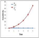
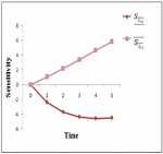
Sensitivities are obtained with the help of Equations (46) to (57). Table 7 displays the sensitivities of the repairable multi-state parallel-series device obtained with regard to time corresponding to different failure rates and repair rates.

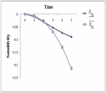
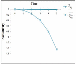
The action of the sensitivity of the device under consideration in relation to various parameters was shown in the Figures 7 to 10.

Table 7 Sensitivity in relation to time corresponding to various parameters

$T$	0	1	2	3	4	5
$\underset{¯}{S_{\underset{¯}{{\lambda }_{32}}}}$	0	0.8102	0.6558	0.5304	0.4286	0.3461
$\underset{¯}{S_{\overline{\lambda {}_{32}}}}$	0	-2.353	-3.6948	-4.3525	-4.559	-4.480
$\underset{¯}{S_{\underset{¯}{{\lambda }_{21}}}}$	0	-0.012	-0.038	-0.0666	-0.0921	-0.1121
$\underset{¯}{S_{\overline{\lambda {}_{21}}}}$	0	-0.0373	-0.1161	-0.2037	-0.2824	-0.3442
$\underset{¯}{S_{\underset{¯}{{\mu }_{12}}}}$	0	-0.0098	-0.0304	-0.0533	-0.0737	-0.0896
$\underset{¯}{S_{\overline{\mu {}_{12}}}}$	0	-0.00098	-0.0033	-0.0061	-0.009	-0.0117
$\overline{S_{\underset{¯}{{\lambda }_{32}}}}$	0	4.1858	11.452	23.170	41.241	68.290
$\overline{S_{\overline{{\lambda }_{32}}}}$	0	1.0505	2.1905	3.3948	4.6243	5.8223
$\overline{S_{\underset{¯}{{\lambda }_{21}}}}$	0	-0.0686	-0.3121	-0.7991	-1.6168	-2.875
$\overline{S_{\overline{{\lambda }_{21}}}}$	0	-0.0440	-0.1860	-0.4794	-0.9762	-1.747
$\overline{S_{\underset{¯}{{\mu }_{12}}}}$	0	-0.0067	-0.0289	-0.0692	-0.1302	-0.2139
$\overline{S_{\overline{{\mu }_{12}}}}$	0	-0.0339	-0.1550	-0.3995	-0.8135	-1.4565

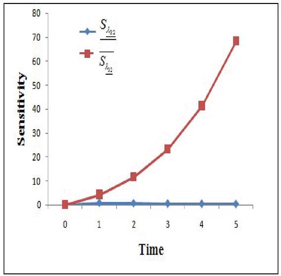
Figure 7 Sensitivities corresponding to ${\underset{¯}{\lambda }}_{32}$ v/s time.

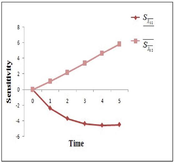
Figure 8 Sensitivities corresponding to ${\overline{\lambda }}_{32}$ v/s time.

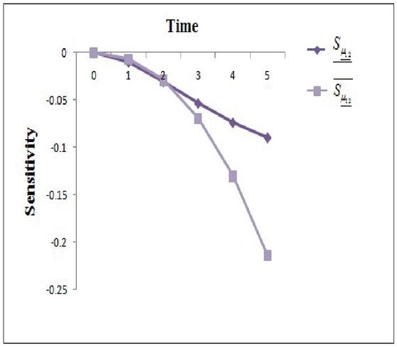
Figure 9 Sensitivities corresponding to ${\underset{¯}{\mu }}_{12}$ v/s time.

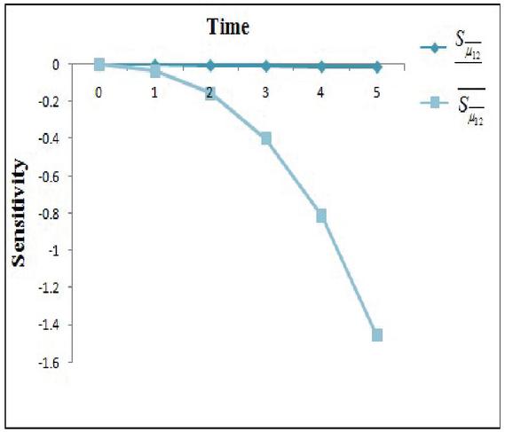
Figure 10 Sensitivities corresponding to ${\underset{¯}{\mu }}_{12}$ v/s time.

7 Results

The present study reveals that both the lower and upper bound reliability is decreasing with the increment in time t. One can easily conclude that as $\underset{¯}{{\lambda }_{32}}$ increases lower bound of MTTF increase and upper bond of MTTF decreases. It is also revealed that as $\overline{{\lambda }_{32}}$ increases lower bound of MTTF decreases and upper bond of MTTF increases rapidly. Also, one can observe that as $\underset{¯}{{\lambda }_{21}}$ increases lower bound of MTTF remains constant and upper bond of MTTF increases. We have also observed that as $\overline{{\lambda }_{21}}$ increases lower bound of MTTF increases and upper bond of MTTF remains constant. It is clear that sensitivity ${\underset{¯}{S}}_{\underset{¯}{{\lambda }_{32}}}$ decreases slowly while sensitivity ${\overline{S}}_{\underset{¯}{{\lambda }_{32}}}$ increases rapidly with increment in time t. By observing the outcome of study, we easily conclude that ${\underset{¯}{S}}_{\underset{¯}{{\lambda }_{32}}}$ decreases with increase in time t, on the other hand ${\overline{S}}_{\underset{¯}{{\lambda }_{32}}}$ increases with the enhancement in time t. Further, results reveal that ${\underset{¯}{S}}_{\underset{¯}{{\lambda }_{21}}}$ and ${\overline{S}}_{\underset{¯}{{\lambda }_{21}}}$ found to be decreasing with increment in time t. ${\underset{¯}{S}}_{\underset{¯}{{\lambda }_{21}}}$ decreases gradually while ${\overline{S}}_{\underset{¯}{{\lambda }_{21}}}$ decreases rapidly with increase in time t. Study also reveals that the sensitivities ${\underset{¯}{S}}_{{\mu }_{12}}$ and ${\overline{S}}_{\underset{¯}{{\mu }_{12}}}$ both decreasing rapidly with the increment in time t. One can further observe that sensitivity ${\underset{¯}{S}}_{{\mu }_{12}}$ decreases very slowly whereas sensitivity ${\overline{S}}_{\underset{¯}{{\mu }_{12}}}$ decreases very fast with the increment in time t.

8 Conclusion

One cannot rule out aleatory and epistemic uncertainties in industrial system. Therefore, it is always a challenge to handle it properly. In the above discussed work an effective approach, namely, IUGF is applied which is fundamentally based on the traditional UGF. It is applicable when there is an uncertainty in the state probabilities of system components. In the current study the system reliability, MTTF and sensitivity of the discussed model have been computed with the use of IUGF approach incorporating Markovian process.

References

[1] Campos, M. A., & Mendonça, A. F. Interval Enclosures for Reliability Metrics. TEMA (São Carlos), 2016; 17(2): 143–172.

[2] Çekyay, B., & Özekici, S. Reliability, MTTF and steady-state availability analysis of systems with exponential lifetimes. Applied Mathematical Modeling, 2015; 39(1): 284–296.

[3] Du, X. Interval reliability analysis. American Society of Mechanical Engineers, International Design Engineering Technical Conferences and Computers and Information in Engineering Conference, 2007; 1103–1109.

[4] Guilani, P. P., Sharifi, M., Niaki, S. T. A., & Zaretalab, A. Reliability evaluation of non-reparable three-state systems using Markov model and its comparison with the UGF and the recursive methods. Reliability Engineering & System Safety, 2014; 129: 29–35.

[5] Gupta, R. K., Bhunia, A. K., & Roy, D. A GA based penalty function technique for solving constrained redundancy allocation problem of series system with interval valued reliability of components. Journal of Computational and Applied Mathematics, 2009; 232(2): 275–284.

[6] Jain, M., & Gupta, R. Optimal replacement policy for a repairable system with multiple vacations and imperfect fault coverage. Computers & Industrial Engineering, 2013; 66(4): 710–719.

[7] Jain, S., Kumar, A., Mandal, S., Ong, J., Poutievski, L., Singh, A., Venkata, S., Wanderer, J., Zhou, J., Zhu, M. and Zolla, J., 2013, August. B4: Experience with a globally deployed software defined WAN. ACM SIGCOMM Computer Communication Review, 2013; 43(4): 3–14.

[8] Kozine, I. O., & Utkin, L. V. Interval-valued finite Markov chains. Reliable computing, 2002; 8(2): 97–113.

[9] Kumar, A., Singh, S. B., & Ram, M. Interval-valued reliability assessment of 2-out-of-4 system. International Conference on Emerging Trends in Communication Technologies; 2016:1–4.

[10] Levitin, G., Xing, L., & Dai, Y. Minimum mission cost cold-standby sequencing in non-repairable multi-phase systems. IEEE Transactions on Reliability, 2014; 63(1): 251–258.

[11] Li, C. Y., Chen, X., Yi, X. S., & Tao, J. Y. Interval-valued reliability analysis of multi-state systems. IEEE Transactions on Reliability, 2011; 60(1): 323–330.

[12] Lisnianski, A., & Ding, Y. Redundancy analysis for repairable multi-state system by using combined stochastic processes methods and universal generating function technique. Reliability Engineering & System Safety, 2009; 94(11): 1788–1795.

[13] Meenakshi, K., & Singh, S. B. Availability Assessment of Multi-State System by Hybrid Universal Generating Function and Probability Intervals. International Journal of Performability Engineering, 2016; 12(4): 321–339.

[14] Negi, S., & Singh, S. B. Reliability analysis of non-repairable complex system with weighted subsystems connected in series. Applied Mathematics and Computation, 2015; 262: 79–89.

[15] Pan, G., Shang, C. X., Liang, Y. Y., Cai, J. Y., & Li, D. Y. Analysis of Interval-Valued Reliability of Multi-State System in Consideration of Epistemic Uncertainty. In International Conference on P2P, Parallel, Grid, Cloud and Internet Computing, 2016; 69–80.

[16] Pokorádi, L. Sensitivity analysis of reliability of Systems with Complex Interconnections. Journal of Loss Prevention in the Process Industries, 2014; 32: 436–442.

[17] Srivastava, M., Nambiar, M., Sharma, S., Karki, S. S., Goldsmith, G., Hegde, M., & Natarajan, R. An inhibitor of non-homologous end-joining abrogates double-strand break repair and impedes cancer progression. 2012; 151(7): 1474–1487.

[18] Wang, K.-H., Yeh, T.-S. & Jian, J.-J. Reliability and sensitivity analysis of a repairable system with imperfect coverage under service pressure condition. Journal of Manufacturing Systems, 2013; 32(2): 357–363.

[19] Wang, W., Xiong, J., & Xie, M. A study of interval analysis for cold-standby system reliability optimization under parameter uncertainty. Computers & Industrial Engineering, 2016; 97: 93–100.

[20] Wang, Y., & Li, L. Effect of uncertainty in both component reliability and load demand on multistate system reliability. IEEE Trans. Rel. 2012; 42(4): 958–969.

[21] Wu, W., Tang, Y., Yu, M., & Jiang, Y. Reliability analysis of a k-out-of-n: G repairable system with single vacation. Applied Mathematical Modeling, 2014; 38(24): 6075–6097.

[22] Xing, L., & Levitin, G. BDD-based reliability evaluation of phased-mission systems with internal/external common-cause failures. Reliability Engineering & System Safety, 2013; 112: 145–153.

[23] Xu, X., Zhang, Z., Xu, D., & Chen, Y. Interval-valued evidence updating with reliability and sensitivity analysis for fault diagnosis. International Journal of Computational Intelligence Systems, 2016; 9(3): 396–415.

[24] Z. W., Huang, H. Z., and Liu, Y. A discrete stress–strength interference model based on universal generating function. Reliability Engineering & System Safety, 2008; 93(10): 1485–1490.

Biographies

Renu received the B.Sc. degree in science from Kumaun University, Nainital, India in 2015 and M.Sc. degree in Mathematics from G. B. Pant University of Agriculture and Technology, Pantnagar, India, in 2017. She has cleared CSIR NET in Mathematics in 2019. She has also been selected for INSPIRE Programme of Government of India from 2012 to 2015. She has been published one research paper in Emerald. Her area of research is Reliability Theory.

Soni Bisht received the B.Sc. and M.Sc. degree in science from H.N.B. Garhwal Central University, Srinagar, India in 2012 and 2014, and the Ph.D. degree major in Mathematics and minor in Computer science from G. B. Pant University of Agriculture and Technology, Pantnagar, India, in 2018. She is currently working as an Assistant Professor in Department of Mathematics, Eternal University, Baru Sahib, Himachal Pradesh in India. She has been published 12 research papers in IEEE Explore, Emerald, International Journal of Mathematical, Engineering and Management Sciences and many other national and international journals of repute and also presented her works at national and international conferences. She has been conferred with “Young Scientist Award” by the Uttarakhand State Council for Science and Technology, Dehradun, in 2018. Her area of research is Reliability Theory, Applied Mathematics, Network Reliability and Parallel and Distributed Systems.

S. B. Singh is a Professor in the Department of Mathematics, Statistics and Computer Science, G. B. Pant University of Agriculture and Technology, Pantnagar (Uttarakhand), India. He has around 25 years of teaching and research experience to Undergraduate and Post Graduate students at different Engineering Colleges and University. Prof. Singh is a member of Indian Mathematical Society, Operations Research Society of India, Member of Advisory board of Intellectual Society for Socio-Techno Welfare (ISST) and National Society for Prevention of Blindness in India and Member of Indian Science Congress Association. He is a regular reviewer of many books and International/National Journals. Prof. Singh has been a member of organizing committee of many international and national conferences and workshops. He is an Editor-in-Chief of the ‘Journal of Reliability and Statistical Studies’. He is member of Editorial board of seven journals and edited books as well. He has authored and coauthored eight books on different courses of Applied/Engineering Mathematics. Prof. Singh has been conferred with five national awards and the Best Teacher Award. He has been included in the special edition of Marquis Who’s Who in the World 2015, USA. His area of research is Reliability Theory/Engineering.

Journal of Reliability and Statistical Studies, Vol. 14, Issue 1 (2021), 81–120.
doi: 10.13052/jrss0974-8024.1415
© 2021 River Publishers