Statistical Inferences on Odd Fréchet Power Function Distribution

Muhammad Ahsan ul Haq¹, Mohammed Albassam², Muhammad Aslam^2,* and Sharqa Hashmi³

¹College of Statistical & Actuarial Sciences, University of the Punjab, Pakistan

Quality Enhancement Cell, National College of Arts, Pakistan

²Department of Statistics, Faculty of Science, King Abdulaziz University, Jeddah 21551, Saudi Arabia

³Lahore College for Women University, Lahore Pakistan

E-mail: ahsanshani36@gmail.com; malbassam@kau.edu.sa; aslam_ravian@hotmail.com; sharqa1972@yahoo.com

*Corresponding Author

Received 23 September 2020; Accepted 09 February 2021; Publication 22 March 2021

Abstract

This article introduces a new unit distribution namely odd Fréchet power (OFrPF) distribution. Numerous properties of the proposed model including reliability analysis, moments, and Rényi Entropy for the proposed distribution. The parameters of the OFrPF distribution are obtained using different approaches such as maximum likelihood, least squares, weighted least squares, percentile, Cramer-von Mises, Anderson-Darling. Furthermore, a simulation was performed to study the performance of the suggested model. We also perform a simulation study to analyze the performances of estimation methods derived. The applications are used to show the practicality of OFrPF distribution using two real data sets. OFrPF distribution performed better than other competitive models.

Keywords: OFr-G family, power function distribution, entropy, estimation methods, data analysis.

1 Introduction

Chosen an appropriate lifetime probability is a major issue for data modeling. However, over the years numerous probability models have been broadly suggested for the analysis of data sets in several areas, medical sciences, actuarial sciences, engineering, finance and insurance, demography, biological sciences, and economics. Sometimes the existing probability distributions do not provide a good fit for more peaked and heavy-tailed data sets. Thus, there is a need to propose a new probability distribution by adding one or more parameter(s). In literature, various approaches are available for the derivation of new families of probability models. The famous among these families are the Weibull-G family (Bourguignon et al., 2014), generalized odd log-logistic-G family (Cordeiro et al., 2016), generalized odd Burr III-G family (Haq et al., 2019), odd Fréchet-G family (Haq and Elgarhy, 2018).

In many applied situations, we have to deal with uncertainty of bounded situations. We frequently experience factors like proportions of a specific trademark, scores of some capacity tests, diverse lists and rates, which lie on interval (0,1) (Cook et al., 2008; Cribari-Neto and Souza, 2013; Gupta and Nadarajah, 2004). For precision, appropriate modeling consider this evidence into account. The unit interval probability distributions are essential for modeling such data sets. Some most useful unit-interval distributions are Topp–Leone distribution (Topp and Leone, 1955), Johnson distribution (Johnson, 1949), Kumaraswamy distribution (Kumaraswamy, 1980), unit-Weibull distribution (J Mazucheli et al., 2018), unit-Lindley distribution (Josmar Mazucheli et al., 2018) and unit modified Burr-III distribution (Haq et al., 2020).

The power function (PF) distribution has many applications in the field of reliability. It was proposed by (Dallas, 1976) using the inverse transformation on the Pareto distribution. The cumulative distribution function (cdf); $G(x)$ and probability density function (pdf); $g(x)$ of power function (PF) distribution are given by

$G(x)=x^{\beta },\&\mathit{\hspace{1em}}g(x)=\beta x^{\beta -1},0<x<1,\beta >0.$

(1)

where $\beta$ is the shape parameter.

Since then, many generalizations of PF distribution are introduced and studied, for example, beta power function by (Cordeiro and dos Santos Brito, 2012), Weibull PF distribution by (Tahir et al., 2016), transmuted PF distribution by (Haq et al., 2016), exponentiated Weibull power function by (Hassan and Assar, 2017), McDonald power function by (Haq et al., 2018), Transmuted Weibull Power function (Haq et al., 2018) and exponentiated transmuted power function by (Usman et al., 2018).

The foundation of this study is the odd Fréchet generated (OFr-G) family (Haq and Elgarhy, 2018). This family is replaced by the cdf

$F(x)=e^{-{\left[\frac{1-G(x)}{G(x)}\right]}^{\theta },}$

(2)

and its related pdf is

$f(x)={\displaystyle \frac{\theta g(x){[1-G(x)]}^{\theta -1}}{G{(x)}^{\theta +1}}}{e}^{-{\left[\frac{1-G(x)}{G(x)}\right]}^{\theta }},0<x<1.$

(3)

where $\theta$ and $\beta$ are the shape parameters.

In this article, we present a new two parameteric distribution (0,1) based on the mixture of Fréchet and power function distribution. The new probability distribution, Fréchet power function distribution, can be applied to define those datasets whose range is 0 to 1. We derive major mathematical properties of OFrPFD and obtain estimators of the its parameters using different estimation approaches. We are motivated to introduce OFrPF distribution because (i) it is capable of modeling bathtub or monotonically increasing hazard rate; (ii) it can be viewed as a suitable distribution for fitting the skewed data. The flexibility of the proposed model is assessed by its applications to two real-life datasets. These applications show that it fitted real-life data better than other three competing lifetime distributions in modeling tensile strength of polyester fibers and rock samples from petroleum data. Additionally, a simulation study is performed which proves the Anderson and Darling (AD) estimators as the best estimation technique among all proposed methods.

2 The Odd Fréchet Power Function Distribution

Let X be a random variable that is OFrPF distribution. The pdf of OFrPF distribution is given as

$f(x)=\theta \beta x^{-(\theta \beta +1)}{[1-x^{\beta }]}^{\theta -1}{e}^{-{\left[\frac{1-x^{\beta }}{x^{\beta }}\right]}^{\theta }},0<x<1,\beta ,\theta >0,$

(4)

The corresponding cdf is

$F(x)=e^{-{\left[\frac{1-x^{\beta }}{x^{\beta }}\right]}^{\theta }}.$

(5)

2.1 Limiting Behavior of Probability Density Function

We observe the following conditions on the probability density function

$\underset{x\to 0}{lim}f(x)$	$=\underset{x\to 0}{lim}\left(\theta \beta x^{-(\theta \beta +1)}{[1-x^{\beta }]}^{\theta -1}{e}^{-{\left[\frac{1-x^{\beta }}{x^{\beta }}\right]}^{\theta }}\right)=0$
$\underset{x\to 1}{lim}f(x)$	$=\underset{x\to 1}{lim}\left(\theta \beta x^{-(\theta \beta +1)}{[1-x^{\beta }]}^{\theta -1}{e}^{-{\left[\frac{1-x^{\beta }}{x^{\beta }}\right]}^{\theta }}\right)$
	$=\{\begin{array}{cc}0\mathit{\hspace{1em}}\hfill & \mathrm{for}\theta >1\hfill \\ \beta \mathit{\hspace{1em}}\hfill & \mathrm{for}\theta =1\hfill \\ \mathrm{\infty }\mathit{\hspace{1em}}\hfill & \mathrm{for}\mathrm{\hspace{0.25em}0}<\theta <1\hfill \end{array}$

From the above, it can be observed the following:

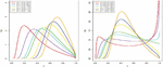
• At origin pdf curve assumes monotonically increasing trend for all values of $\beta >0$ and $\theta >0$.

• The pdf is modal, reaching the point $\beta$ and possibly increasing trend at $x\to 1$ for all values of $\beta >0$ and specified values of $\theta$.

the pdf curves of OFrPF distribution are given in Figure 1. It is observed that the pdf curve may assume positively skewed and negatively skewed trends.

Figure 1 Plots for probability density functions of the OFrPF distribution.

3 Properties of OFrPF Distribution

In this section, we discuss some mathematical properties of OFrPF distribution.

3.1 Quantile Function

Using Equation (5), the OFrPFD can be easily obtained by

$$X={[1+{(-\log (U))}^{\frac{1}{\theta }}]}^{-\frac{1}{\beta }},$$

where $U$ follows Uniform (0, 1). The $p$th quantile of OFrPFD is given by

$$x_p={[1+{(-\log (p))}^{\frac{1}{\theta }}]}^{-\frac{1}{\beta }}.$$

The median of OFrPF distribution can be obtained as

$$x_{0.5}={\left[1+{\left(-\log \left(\frac{1}{2}\right)\right)}^{\frac{1}{\theta }}\right]}^{-\frac{1}{\beta }}.$$

3.2 Mixture Representation

Using the exponential expansion, the pdf (4) can be written as

$$f(x)=\theta \beta x^{-(\theta \beta +1)}{[1-x^{\beta }]}^{\theta -1}\sum _{j=0}^{\mathrm{\infty }}\frac{{(-1)}^j}{j!}{\left(\frac{1-x^{\beta }}{x^{\beta }}\right)}^{\theta j},$$

For $\beta >0$ and $|z|<1$, the binomial theorem can be expressed as

$${(1-z)}^{\beta -1}=\sum _{i=0}^{\mathrm{\infty }}{(-1)}^i\left(\begin{array}{c}\hfill \beta -1\hfill \\ \hfill i\hfill \end{array}\right)z^i.$$

The pdf can be written as

$f(x)=\theta \beta {\displaystyle \sum _{j=0}^{\mathrm{\infty }}}{\displaystyle \sum _{k=0}^{\mathrm{\infty }}}{\displaystyle \frac{{(-1)}^{j+k}}{j!}}\left({\displaystyle \genfrac{}{}{0.0pt}{}{\theta j+\theta -1}{k}}\right)x^{\beta k-\theta \beta (j+1)-1}.$

(6)

3.3 Moments

Using the pdf in Equation (6), the $r$th moment of OFrPFD can be obtained as follows:

${\mu }_r^{\prime }=E(X^r)={\displaystyle \sum _{j=0}^{\mathrm{\infty }}}{\displaystyle \sum _{k=0}^{\mathrm{\infty }}}{\displaystyle \frac{{(-1)}^{j+k}}{j!}}\left({\displaystyle \genfrac{}{}{0.0pt}{}{\theta j+\theta -1}{k}}\right)\left[{\displaystyle \frac{\theta \beta }{(r+\beta k-\theta \beta (j+1))}}\right].$

(7)

Table 1 presents the numerical values of ${\mu }_1,{\mu }_2^{\prime },{\mu }_3^{\prime },{\mu }_4^{\prime },$ variance (V(X)), coefficient of skewness (CS), and coefficient of kurtosis (CK) for selected values of the parameters.

Table 1 Moments, variance, skewness, and kurtosis of the OFrPFD

Parameters		${\mu }_1^{\prime }$	${\mu }_2^{\prime }$	${\mu }_3^{\prime }$	${\mu }_4^{\prime }$	V(X)	CS	CK
$\theta =1.0$	$\beta =0.5$	0.4037	0.2339	0.1617	0.1229	0.0710	0.5254	2.1580
$\theta =1.0$	$\beta =0.7$	0.4980	0.3101	0.2201	0.1693	0.0620	0.2540	1.9808
$\theta =1.0$	$\beta =1.0$	0.5964	0.4037	0.2982	0.2339	0.0480	0.0171	1.9815
$\theta =1.0$	$\beta =1.5$	0.6970	0.5174	0.4037	0.3273	0.0316	$-$0.1938	2.1092
$\theta =1.5$	$\beta =0.5$	0.3606	0.1721	0.0994	0.0651	0.0421	0.8166	2.9757
$\theta =1.5$	$\beta =0.7$	0.4670	0.2552	0.1575	0.1066	0.0371	0.5252	2.5386
$\theta =1.5$	$\beta =1.0$	0.5763	0.3606	0.2419	0.1721	0.0284	0.2937	2.3500
$\theta =1.5$	$\beta =1.5$	0.6859	0.4887	0.3606	0.2744	0.0183	0.1037	2.3035
$\theta =2.0$	$\beta =0.5$	0.3346	0.1389	0.0689	0.0393	0.0269	1.0133	3.7425
$\theta =2.0$	$\beta =0.7$	0.4470	0.2240	0.1244	0.0755	0.0241	0.7139	3.0834
$\theta =2.0$	$\beta =1.0$	0.5622	0.3346	0.2103	0.1389	0.0186	0.4888	2.7486
$\theta =2.0$	$\beta =1.5$	0.6768	0.4700	0.3346	0.2441	0.0119	0.3123	2.5842

3.4 Rényi Entropy

The entropy of a random variable $X$ is an index of diversity or uncertainty. The Rényi entropy, say $R{E}_X$, is defined as

$$R{E}_X=\frac{1}{\delta -1}\log \left({\int }_{-\mathrm{\infty }}^{\mathrm{\infty }}f{(x)}^{\delta }\mathit{d}x\right),\delta \ge 0,\delta \ne 1.$$

As $\alpha \to \mathrm{\infty }$, the Rényi entropy is increasingly defined by the events of highest probability whereas $\delta \to 0$, the Rényi entropy increasingly weighs all events equally, irrespective of their probabilities. Using the pdf in Equation (4), the Rényi entropy of $X$ can be obtained as follows:

$$R{E}_X=\frac{1}{\delta -1}\log \left({\int }_{-\mathrm{\infty }}^{\mathrm{\infty }}{\left(\theta \beta x^{-(\theta \beta +1)}{[1-x^{\beta }]}^{\theta -1}{e}^{-{\left[\frac{1-x^{\beta }}{x^{\beta }}\right]}^{\theta }}\right)}^{\delta }\mathit{d}x\right)$$

Consider an integral part

${\displaystyle {\int }_{-\mathrm{\infty }}^{\mathrm{\infty }}}f{(x)}^{\delta }\mathit{d}x$	$={\displaystyle \sum _{j=0}^{\mathrm{\infty }}}{\displaystyle \sum _{k=0}^{\mathrm{\infty }}}{\displaystyle \frac{{(-1)}^{j+k}}{j!}}\left({\displaystyle \genfrac{}{}{0.0pt}{}{\delta (\theta j+\theta -1)}{k}}\right)$
	$\mathrm{\hspace{1em}}\times \left[{\displaystyle \frac{{(\theta \beta )}^{\delta }}{\delta [\beta k-\theta \beta (j+1)-1]+1}}\right],$

The final form of RE${}_x$ is

$R{E}_X$	$={\displaystyle \frac{1}{\delta -1}}\log \{{\displaystyle \sum _{j=0}^{\mathrm{\infty }}}{\displaystyle \sum _{k=0}^{\mathrm{\infty }}}{\displaystyle \frac{{(-1)}^{j+k}}{j!}}\left({\displaystyle \genfrac{}{}{0.0pt}{}{\delta (\theta j+\theta -1)}{k}}\right)$
	$\mathrm{\hspace{1em}}\times \left[{\displaystyle \frac{{(\theta \beta )}^{\delta }}{\delta [\beta k-\theta \beta (j+1)-1]+1}}\right]\}.$	(8)

Table 2 Values of the Rényi entropy of the OFrPF distribution for some parameter values

$\delta$	$\theta$	$\beta$	Rényi Entropy
0.5	1.0	0.5	0.0529235
0.5	1.0	0.7	0.0676647
0.5	1.0	1.0	0.1604457
0.5	1.0	1.5	0.3459248
1.5	1.5	0.5	0.3893141
1.5	1.5	0.7	0.3630736
1.5	1.5	1.0	0.4555590
2.0	1.5	1.5	0.6601460
2.0	2.0	0.5	0.7022644
2.0	2.0	0.7	0.6602884
2.0	2.0	1.0	0.7403408
2.0	2.0	1.5	0.9349705

From Table 2, it can be seen that the Rényi entropy increases as an increase occurs in parameter values. Thus, its parameters effect the Rényi entropy. Shannon’s entropy is a special case of Rényi entropy as $\delta \to 1$. Entropies quantify the uncertainty or randomness of a structure.

4 Reliability Characteristics

4.1 Survival, Hazard (Failure) Rate Function and Cumulative Hazard Function

The survival function, hazard rate function (hrf) and cumulative hazard rate function of X is given, respectively as follows:

$S(x)$	$=1-e^{-{[\frac{1-x^{\beta }}{x^{\beta }}]}^{\theta }},$	(9)
$h(x)$	$={\displaystyle \frac{\theta \beta x^{-(\theta \beta +1)}{[1-x^{\beta }]}^{\theta -1}{e}^{-{[\frac{1-x^{\beta }}{x^{\beta }}]}^{\theta }}}{1-e^{-{[\frac{1-x^{\beta }}{x^{\beta }}]}^{\theta }}}},$	(10)

and

$H(x)=-\log \{1-e^{-{[\frac{1-x^{\beta }}{x^{\beta }}]}^{\theta }}\}.$

(11)

4.2 Limiting Behavior of Hazard Rate Function

We observe the following conditions on hazard rate function

$\underset{x\to 0}{lim}h(x)$	$=\underset{x\to 0}{lim}\left({\displaystyle \frac{\theta \beta x^{-(\theta \beta +1)}{[1-x^{\beta }]}^{\theta -1}{e}^{-{[\frac{1-x^{\beta }}{x^{\beta }}]}^{\theta }}}{1-e^{-{[\frac{1-x^{\beta }}{x^{\beta }}]}^{\theta }}}}\right)=0$
$\underset{x\to 1}{lim}h(x)$	$=\underset{x\to 1}{lim}\left({\displaystyle \frac{\theta \beta x^{-(\theta \beta +1)}{[1-x^{\beta }]}^{\theta -1}{e}^{-{[\frac{1-x^{\beta }}{x^{\beta }}]}^{\theta }}}{1-e^{-{[\frac{1-x^{\beta }}{x^{\beta }}]}^{\theta }}}}\right)=\mathrm{\infty }$

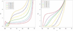
It is observed that the hrf has an increasing trend for all values of parameters.

Some curves of hrf of the OFrPFD are plotted in Figure 2. It is observed that the hrf can be increasing shapes.

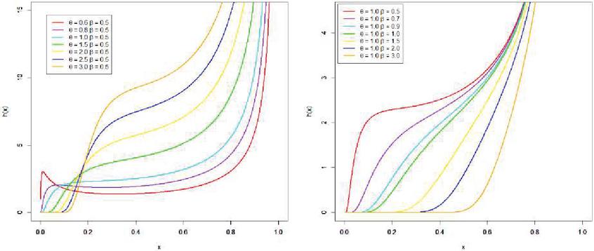
Figure 2 Plots for the hrf of the OFrPFD.

4.3 Mean Residual Life

The aging of the process is studied using the mean residual life (MRL) is given as

$$\mu (t)=\frac{1}{S(t)}{\int }_t^{\mathrm{\infty }}xf(x)\mathit{d}x-t,t>0$$

Using the pdf in Equation (4), the MRL of $X$ can be obtained as follows

$\mu (t)$	$={\displaystyle \frac{\theta \beta }{1-e^{-{[\frac{1-t^{\beta }}{t^{\beta }}]}^{\theta }}}}{\displaystyle \sum _{j=0}^{\mathrm{\infty }}}{\displaystyle \sum _{k=0}^{\theta j+\theta -1}}{\displaystyle \frac{{(-1)}^{j+k}}{j!}}\left({\displaystyle \genfrac{}{}{0.0pt}{}{\theta j+\theta -1}{k}}\right)$
	$\mathrm{\hspace{1em}}\times {\displaystyle {\int }_t^1}{x}^{\beta k-\theta \beta (j+1)}\mathit{d}x-t$
$\mu (t)$	$={\displaystyle \frac{\theta \beta }{1-e^{-{[\frac{1-t^{\beta }}{t^{\beta }}]}^{\theta }}}}{\displaystyle \sum _{j=0}^{\mathrm{\infty }}}{\displaystyle \sum _{k=0}^{\theta j+\theta -1}}{\displaystyle \frac{{(-1)}^{j+k}}{j!}}\left({\displaystyle \genfrac{}{}{0.0pt}{}{\theta j+\theta -1}{k}}\right)$
	$\mathrm{\hspace{1em}}\times \left[{\displaystyle \frac{1-t^{1+k\beta -\theta \beta (1+j)}}{k\beta -\theta \beta (1+j)+1}}\right]-t$	(12)

4.4 Mean Inactivity Time

The mean inactivity time (MIT) function has much application in various fields and derived for a random variable $X$ as

$$m(t)=t-\frac{1}{G(t)}{\int }_0^{t}xf(x)\mathit{d}x,t>0$$

Using the pdf in Equation (4), the MIT of $X$ can be given as follows

$m(t)$	$=t-{\displaystyle \frac{\theta \beta }{e^{-{[\frac{1-t^{\beta }}{t^{\beta }}]}^{\theta }}}}{\displaystyle \sum _{j=0}^{\mathrm{\infty }}}{\displaystyle \sum _{k=0}^{\theta j+\theta -1}}{\displaystyle \frac{{(-1)}^{j+k}}{j!}}\left({\displaystyle \genfrac{}{}{0.0pt}{}{\theta j+\theta -1}{k}}\right)$
	$\mathrm{\hspace{1em}}\times {\displaystyle {\int }_0^t}{x}^{\beta k-\theta \beta (j+1)}\mathit{d}x$
$m(t)$	$=t-{\displaystyle \frac{\theta \beta }{e^{-{[\frac{1-t^{\beta }}{t^{\beta }}]}^{\theta }}}}{\displaystyle \sum _{j=0}^{\mathrm{\infty }}}{\displaystyle \sum _{k=0}^{\theta j+\theta -1}}{\displaystyle \frac{{(-1)}^{j+k}}{j!}}\left({\displaystyle \genfrac{}{}{0.0pt}{}{\theta j+\theta -1}{k}}\right)$
	$\mathrm{\hspace{1em}}\times \left[{\displaystyle \frac{t^{1+k\beta -\theta \beta (1+j)}}{1+k\beta -\theta \beta (1+j)}}\right]$	(13)

5 Order Statistics

Let $X_1,X_2,\mathrm{\dots },X_n$ be a random sample from the OFrPF model of distributions and let $X_{1:n},X_{2:n},\mathrm{\dots },X_{n:n}$ be relevant order statistics. The pdf of $i$th order statistics say $X_{i:n}$, can be written as

$$f_{i:n}(x)=\frac{f(x)}{B(i,n-i+1)}\sum _{v=0}^{n-i}{(-1)}^v\left(\begin{array}{c}\hfill n-i\hfill \\ \hfill v\hfill \end{array}\right)F^{v+i-1}(x),$$

where $B(\cdot ,\cdot )$ is the beta function, using (5) and (9), we get

$f_{i:n}(x)$	$={\displaystyle \frac{\theta \beta {\sum }_{j=0}^{\mathrm{\infty }}{\sum }_{k=0}^{\mathrm{\infty }}\frac{{(-1)}^{j+k}}{j!}\left(\genfrac{}{}{0.0pt}{}{\theta j+\theta -1}{k}\right)x^{\beta k-\theta \beta (j+1)-1}}{B(i,n-i+1)}}{\displaystyle \sum _{v=0}^{n-i}}{(-1)}^v$
	$\mathrm{\hspace{1em}}\times \left(\begin{array}{c}\hfill n-i\hfill \\ \hfill v\hfill \end{array}\right)e^{-(v+i-1){[\frac{1-x^{\beta }}{x^{\beta }}]}^{\theta }}$

The pdf of $X_{i:n}$ can be expressed as

$f_{i:n}(x)$	$=\theta \beta {\displaystyle \sum _{v=0}^{n-i}}{\displaystyle \sum _{j,k=0}^{\mathrm{\infty }}}{\eta }_k{\displaystyle \frac{{(-1)}^v}{B(i,n-i+1)}}$
	$\mathrm{\hspace{1em}}\times \left(\begin{array}{c}\hfill n-i\hfill \\ \hfill v\hfill \end{array}\right)x^{\beta k-\theta \beta (j+1)-1}{e}^{-(v+i-1){[\frac{1-x^{\beta }}{x^{\beta }}]}^{\theta }}$

where

${\eta }_k$	$={\displaystyle \frac{{(-1)}^{j+k}}{j!}}\left({\displaystyle \genfrac{}{}{0.0pt}{}{\theta j+\theta -1}{k}}\right)$
$f_{i:n}(x)$	$=\theta {\displaystyle \sum _{v=0}^{n-i}}{\displaystyle \sum _{j,k=0}^{\mathrm{\infty }}}{\eta }_k{\rho }_{i,v}{g}_{X_{(i)}}(x,\beta )G_{X_{(i)}}{(x,\beta )}^{j+k}$

where

$${\rho }_{i,v}=\frac{{(-1)}^v}{B(i,n-i+1)}\left(\begin{array}{c}\hfill n-i\hfill \\ \hfill v\hfill \end{array}\right)$$

The moments of $X_{i:n}$ can be calculated as

$$E(X_{i:n}^q)=\theta \sum _{v=0}^{n-i}\sum _{j,k=0}^{\mathrm{\infty }}{\eta }_k{\rho }_{i,v}{\tau }_{q,j+k}.$$

Where ${\tau }_{q,j+k}$ is probability generated moments of $g(x)$.

6 Parameter Estimation

In this section, we define six estimation approaches for estimating $\theta$, and $\beta$ parameters of OFrPF distribution. For all the methods of estimation, we assume that $x_1,x_2,\mathrm{\dots },x_n$ is a random sample of size $n$ from OFrPF distribution, with unknown parameters $\theta$ and $\beta$. Besides, consider that $x_{(1)},x_{(2)},\mathrm{\dots },x_{(n)}$ denote the corresponding order samples.

6.1 ML Estimation

Here, we consider the estimation of unknown parameters using the maximum likelihood method. The MLE approach is most ideal due to its attractive properties (Lehmann and Casella, 2006). The log-likelihood function for the vector of parameters $\mathrm{\Phi }={(\theta ,\beta )}^T$ can be expressed as

$l$	$=n\log (\theta \beta )-(\theta \beta +1){\displaystyle \sum _{i=1}^n}\log x_i+(\theta -1){\displaystyle \sum _{i=1}^n}\log (1-x_i{}^{\beta })$
	$\mathrm{\hspace{1em}}+{\displaystyle \sum _{i=1}^n}\log \left[\exp \left\{-{\left({\displaystyle \frac{1-x_i{}^{\beta }}{x_i{}^{\beta }}}\right)}^{\theta }\right\}\right].$

The elements of the score vector $U(\mathrm{\Phi })$ are given by

$U_{\theta }$	$={\displaystyle \frac{n}{\theta }}-\beta {\displaystyle \sum _{i=1}^n}\log (x_i)+{\displaystyle \sum _{i=1}^n}\log (1-x_i{}^{\beta })$
	$\mathrm{\hspace{1em}}-{\displaystyle \sum _{i=1}^n}\left[\log (x_i^{-\beta }-1)\right]{(x_i^{-\beta }-1)}^{\theta },$
$U_{\beta }$	$={\displaystyle \frac{n}{\beta }}-\theta {\displaystyle \sum _{i=1}^n}\log (x_i)-(\theta -1){\displaystyle \sum _{i=1}^n}{\displaystyle \frac{x_i{}^{\beta }\log (x_i)}{1-x_i{}^{\beta }}}$
	$\mathrm{\hspace{1em}}-\theta {\displaystyle \sum _{i=1}^n}\left[\log (x_i){(x_i^{-\beta }-1)}^{\theta }\right]{(x_i^{-\beta }-1)}^{-1}$

Setting these two non-linear equations to zero and solving them simultaneously yield the MLEs of the model parameters. These equations can be solved numerically using the Newton-Raphson algorithm or the Bisection method. Computer software such as R Language, Mathematica, MATLAB can be used for this purpose.

Based on the asymptotic normal approximation for $(\widehat{\theta },\widehat{\beta })$, interval estimation can be easily performed from the observed information matrix $J_n(\theta ,\beta ).$ The Information matrix is defined as

$J_n(\theta ,\beta )=-\left[\begin{array}{cc}{J}_{\theta \theta }\mathit{\hspace{1em}}\hfill & J_{\theta \beta }\hfill \\ J_{\beta \theta }\mathit{\hspace{1em}}\hfill & J_{\beta \beta }\hfill \end{array}\right]=-\left[\begin{array}{cc}{\displaystyle \frac{{\partial }^2}{\partial {\theta }^2}}\log L(\theta ,\beta )\mathit{\hspace{1em}}\hfill & {\displaystyle \frac{{\partial }^2}{\partial \theta \partial \beta }}\log L(\theta ,\beta )\hfill \\ {\displaystyle \frac{{\partial }^2}{\partial \beta \partial \theta }}\log L(\theta ,\beta )\mathit{\hspace{1em}}\hfill & {\displaystyle \frac{{\partial }^2}{\partial {\beta }^2}}\log L(\theta ,\beta )\hfill \end{array}\right],$

where

$J_{\theta \theta }$	$=-{\displaystyle \frac{n}{{\theta }^2}}-{\displaystyle \sum _{i=1}^n}{\left[\log (x_i^{-\beta }-1)\right]}^2{(x_i^{-\beta }-1)}^{\theta }$
$J_{\theta \beta }$	$=-{\displaystyle \sum _{i=1}^n}\log (x_i)-{\displaystyle \sum _{i=1}^n}{\displaystyle \frac{{(x_i^{-\beta }-1)}^{\theta }\log (x_i)(1+\theta \log (x_i^{-\beta }-1))}{x_i^{\beta }-1}}$
	$\mathrm{\hspace{1em}}+{\displaystyle \sum _{i=1}^n}{\displaystyle \frac{x_i^{\beta }\log (x_i)}{x_i^{\beta }-1}}$
$J_{\beta \beta }$	$=-{\displaystyle \frac{n}{{\beta }^2}}-(\theta -1){\displaystyle \sum _{i=1}^n}{\displaystyle \frac{x_i^{\beta }{(\log x_i)}^2}{{(x_i^{\beta }-1)}^2}}$
	$\mathrm{\hspace{1em}}+\theta {\displaystyle \sum _{i=1}^n}{\displaystyle \frac{{(x_i^{-\beta }-1)}^{\theta }(x_i^{\beta }-\theta ){(\log x_i)}^2}{{(x_i^{\beta }-1)}^2}}$

The observed covariance matrix is the inverse of $J_n(\theta ,\beta ),J_n^{-1}(\theta ,\beta ),$ and the diagonal elements of $J_n^{-1}(\widehat{\theta },\widehat{\beta })$ are the variances of $\widehat{\theta }$ and $\widehat{\beta }$, which denote by $Var(\widehat{\theta })$ and $Var(\widehat{\beta })$, respectively. Then, the asymptotic $(1-\alpha )100\%$ confidence intervals for $\theta$ and $\beta$ are $\widehat{\theta }\pm Z_{\alpha /2}\sqrt{Var(\widehat{\theta })}$ & $\widehat{\beta }\pm Z_{\alpha /2}\sqrt{Var(\widehat{\beta })}$, where $Z_{\alpha /2}$ is the upper $(\alpha /2)th$ percentile of the standard normal distribution.

6.2 Method of Least Square and Weighted Least Square Estimation

The least-square estimates of $\theta$ and $\beta$ can be determined by minimizing the least square function defined by

$$LS(\theta ,\beta )=\sum _{i=1}^n{\left[\exp \left\{-{\left(\frac{1-x_{i:n}{}^{\beta }}{x_{i:n}{}^{\beta }}\right)}^{\theta }\right\}-\frac{i}{n+1}\right]}^2.$$

The WLSEs of $\theta$ and $\beta$ can be determined by minimizing the function:

$WLSEs(\theta ,\beta )$	$={\displaystyle \sum _{i=1}^n}{\displaystyle \frac{{(n+1)}^2(n+2)}{i(n-i+1)}}$
	$\mathrm{\hspace{1em}}\times {\left[\exp \left\{-{\left({\displaystyle \frac{1-x_{i:n}{}^{\beta }}{x_{i:n}{}^{\beta }}}\right)}^{\theta }\right\}-{\displaystyle \frac{i}{n+1}}\right]}^2.$

6.3 Anderson and Darling (AD) Estimation

The Anderson and Darling estimates (ADEs) of $\theta$ and $\beta$ can be obtained by minimizing the function given by

$ADEs(\theta ,\beta )$	$=-n-{\displaystyle \frac{1}{n}}{\displaystyle \sum _{i=1}^n}(2i-1)$
	$\mathrm{\hspace{1em}}\times \{\log F(x_{i:n};\theta ,\beta )+\log \overline{F}(x_{n+1-i:n};\theta ,\beta )\},$

where $\overline{F}(x)=1-F(x)$.

6.4 Cramer–von Mises Minimum (CVM) Distance Estimation

The CVM estimators are obtained by minimizing

$$CVMEs(\theta ,\beta )=\frac{1}{12n}+\sum _{i=1}^n{\left[\exp \left\{-{\left(\frac{1-x_{i:n}{}^{\beta }}{x_{i:n}{}^{\beta }}\right)}^{\theta }\right\}-\frac{2i-1}{2n}\right]}^2.$$

6.5 Percentile Estimation

$U(\theta ,\beta )={\displaystyle \sum _{i=1}^n}{[x_{i:n}-Q(p_i;\theta ,\beta )]}^2={\displaystyle \sum _{i=1}^n}{\left[x_{i:n}-{\left[1+{(-\log p_i)}^{\frac{1}{\theta }}\right]}^{-\frac{1}{\beta }}\right]}^2,$

where $p_i=(i+1)/n$. Thus, the percentile estimates obtained through the following equations $\partial U(\theta ,\beta )/\partial \theta =0$ and $\partial U(\theta ,\beta )/\partial \beta =0$, where

$$\frac{\partial U(\theta ,\beta )}{\partial \theta }=2\sum _{i=1}^n{\eta }_i^{(1)}(\theta ,\beta )\left[x_{i:n}-{\left[1+{(-\log p_i)}^{\frac{1}{\theta }}\right]}^{-\frac{1}{\beta }}\right]$$

and

$$\frac{\partial U(\theta ,\beta )}{\partial \beta }=2\sum _{i=1}^n{\eta }_i^{(2)}(\theta ,\beta )\left[x_{i:n}-{\left[1+{(-\log p_i)}^{\frac{1}{\theta }}\right]}^{-\frac{1}{\beta }}\right],$$

where

$${\eta }_i^{(1)}(\theta ,\beta )=\frac{{(1+{(-\log p_i)}^{\frac{1}{\theta }})}^{-1-\frac{1}{\beta }}{(-\log p_i)}^{\frac{1}{\theta }}\mathrm{Log}[-\log p_i]}{2\beta {\theta }^2\sqrt{{(1+{(-\log p_i)}^{\frac{1}{\theta }})}^{-1/\beta }}},$$

and

$${\eta }_i^{(2)}(\theta ,\beta )=\frac{\sqrt{{(1+{(-\log p_i)}^{\frac{1}{\theta }})}^{-1/\beta }}\mathrm{Log}[1+{(-\log p_i)}^{\frac{1}{\theta }}]}{2{\beta }^2}.$$

These expressions are not explicit and R-language is used to obtain their results numerically.

7 Simulation

In this section, the efficiency of the proposed distribution is examined through the simulation analysis. A Monte Carlo simulation study is provided to investigate the performance of estimators of different estimation techniques discussed above. We generate $N=10000$ random samples of size $n=20$, 50, 100, and from OFrPF distribution. All the computations are obtained by utilizing the R-Language (R Development Core Team, 2019). Seven sets of the parameters are considered as: $\{\theta =0.5,\beta =0.3\},\{\theta =0.5,\beta =1.0\},\{\theta =1.0,\beta =1.5\},\{\theta =1.5,\beta =1.5\}$ and $\{\theta =2.0,\beta =1.5\}$. This procedure is conducted by computing the average absolute bias and the mean square error (MSE), which are given by

$Bias(\mathrm{\Phi })$	$={\displaystyle \frac{1}{N}}{\displaystyle \sum _{j=1}^N}({\widehat{\mathrm{\Phi }}}_i-\mathrm{\Phi })\mathit{\hspace{1em}}\&\mathit{\hspace{1em}}MSE={\displaystyle \frac{1}{N}}{\displaystyle \sum _{j=1}^N}{({\widehat{\mathrm{\Phi }}}_i-\mathrm{\Phi })}^2,$
	$\mathrm{\hspace{1em}}\mathrm{for}i=1,2,3\mathrm{\dots }$

The results obtained are given in Tables 3–7.

Table 3 Simulation results for ${\mathbf{\Phi }}^T=(\theta =0.5,\beta =0.3)$

n	Estimates	MLE	ADE	CVME	OLSE	WLSE	PE
20	$E(\widehat{\theta })$	0.53623	0.51503	0.54358	0.50700	0.51032	0.50534
	$E(\widehat{\beta })$	0.32639	0.32018	0.32935	0.32228	0.32006	0.31598
	$Bias(\widehat{\theta })$	0.03623	0.01503	0.04358	0.00700	0.01032	0.00534
	$Bias(\widehat{\beta })$	0.02639	0.02018	0.02935	0.02228	0.02006	0.01598
	$Var(\widehat{\theta })$	0.01503	0.01435	0.02111	0.01789	0.01667	0.02391
	$Var(\widehat{\beta })$	0.00960	0.01084	0.01558	0.01565	0.01309	0.02659
	$MSE(\widehat{\theta })$	0.01634	0.01458	0.02301	0.01794	0.01678	0.02394
	$MSE(\widehat{\beta })$	0.01030	0.01125	0.01644	0.01615	0.01349	0.02685
50	$E(\widehat{\theta })$	0.51357	0.50482	0.51607	0.50166	0.50527	0.50248
	$E(\widehat{\beta })$	0.31012	0.30769	0.31149	0.30760	0.30740	0.30728
	$Bias(\widehat{\theta })$	0.01357	0.00482	0.01607	0.00166	0.00527	0.00248
	$Bias(\widehat{\beta })$	0.01012	0.00769	0.01149	0.00760	0.00740	0.00728
	$Var(\widehat{\theta })$	0.00520	0.00526	0.00663	0.00608	0.00560	0.00864
	$Var(\widehat{\beta })$	0.00301	0.00353	0.00460	0.00434	0.00379	0.00841
	$MSE(\widehat{\theta })$	0.00538	0.00528	0.00689	0.00608	0.00563	0.00865
	$MSE(\widehat{\beta })$	0.00311	0.00359	0.00473	0.00440	0.00384	0.00846
100	$E(\widehat{\theta })$	0.50717	0.50318	0.50813	0.50238	0.50298	0.50075
	$E(\widehat{\beta })$	0.30445	0.30413	0.30553	0.30339	0.30381	0.30248
	$Bias(\widehat{\theta })$	0.00717	0.00318	0.00813	0.00238	0.00298	0.00075
	$Bias(\widehat{\beta })$	0.00445	0.00413	0.00553	0.00339	0.00381	0.00248
	$Var(\widehat{\theta })$	0.00234	0.00262	0.00312	0.00303	0.00268	0.00426
	$Var(\widehat{\beta })$	0.00134	0.00169	0.00211	0.00204	0.00175	0.00389
	$MSE(\widehat{\theta })$	0.00239	0.00263	0.00319	0.00304	0.00269	0.00426
	$MSE(\widehat{\beta })$	0.00136	0.00171	0.00214	0.00205	0.00176	0.00390
200	$E(\widehat{\theta })$	0.50303	0.50160	0.50339	0.50088	0.50127	0.50096
	$E(\widehat{\beta })$	0.30254	0.30224	0.30325	0.30165	0.30242	0.30171
	$Bias(\widehat{\theta })$	0.00303	0.00160	0.00339	0.00088	0.00127	0.00096
	$Bias(\widehat{\beta })$	0.00254	0.00224	0.00325	0.00165	0.00242	0.00171
	$Var(\widehat{\theta })$	0.00120	0.00129	0.00150	0.00150	0.00127	0.00205
	$Var(\widehat{\beta })$	0.00065	0.00080	0.00101	0.00099	0.00083	0.00183
	$MSE(\widehat{\theta })$	0.00121	0.00129	0.00151	0.00150	0.00127	0.00205
	$MSE(\widehat{\beta })$	0.00066	0.00081	0.00102	0.00099	0.00084	0.00183

Table 4 Simulation results for ${\mathbf{\Phi }}^T=(\theta =0.5,\beta =1.0)$

n	Estimates	MLE	ADE	CVME	OLSE	WLSE	PE
20	$E(\widehat{\theta })$	0.53625	0.51618	0.54449	0.5069	0.51181	0.50126
	$E(\widehat{\beta })$	1.09350	1.06242	1.10698	1.07028	1.06976	1.08592
	$Bias(\widehat{\theta })$	0.03625	0.01618	0.04449	0.00690	0.01181	0.00126
	$Bias(\widehat{\beta })$	0.09350	0.06242	0.10698	0.07028	0.06976	0.08592
	$Var(\widehat{\theta })$	0.01537	0.01456	0.02133	0.01831	0.01626	0.02007
	$Var(\widehat{\beta })$	0.11230	0.11425	0.18845	0.16627	0.14981	0.26906
	$MSE(\widehat{\theta })$	0.01668	0.01482	0.02331	0.01836	0.01640	0.02007
	$MSE(\widehat{\beta })$	0.12104	0.11815	0.19989	0.17121	0.15468	0.27644
50	$E(\widehat{\theta })$	0.51344	0.50596	0.51625	0.50261	0.50499	0.50239
	$E(\widehat{\beta })$	1.03076	1.02364	1.04275	1.02384	1.02887	1.03186
	$Bias(\widehat{\theta })$	0.01344	0.00596	0.01625	0.00261	0.00499	0.00239
	$Bias(\widehat{\beta })$	0.03076	0.02364	0.04275	0.02384	0.02887	0.03186
	$Var(\widehat{\theta })$	0.00508	0.00529	0.00657	0.00627	0.00554	0.00773
	$Var(\widehat{\beta })$	0.03157	0.03890	0.05424	0.04811	0.04364	0.05766
	$MSE(\widehat{\theta })$	0.00526	0.00533	0.00683	0.00628	0.00556	0.00774
	$MSE(\widehat{\beta })$	0.03252	0.03946	0.05607	0.04868	0.04447	0.05868
100	$E(\widehat{\theta })$	0.50693	0.50368	0.50863	0.50167	0.50317	0.50047
	$E(\widehat{\beta })$	1.01570	1.01191	1.01732	1.01030	1.01357	1.01220
	$Bias(\widehat{\theta })$	0.00693	0.00368	0.00863	0.00167	0.00317	0.00047
	$Bias(\widehat{\beta })$	0.01570	0.01191	0.01732	0.01030	0.01357	0.01220
	$Var(\widehat{\theta })$	0.00241	0.00258	0.00309	0.00303	0.00264	0.00392
	$Var(\widehat{\beta })$	0.01439	0.01851	0.02291	0.02242	0.01906	0.02496
	$MSE(\widehat{\theta })$	0.00246	0.00259	0.00316	0.00303	0.00265	0.00392
	$MSE(\widehat{\beta })$	0.01464	0.01865	0.02321	0.02253	0.01924	0.02511
200	$E(\widehat{\theta })$	0.50330	0.50125	0.50397	0.50019	0.50156	0.50065
	$E(\widehat{\beta })$	1.00855	1.00754	1.00936	1.00542	1.00612	1.00711
	$Bias(\widehat{\theta })$	0.00330	0.00125	0.00397	0.00019	0.00156	0.00065
	$Bias(\widehat{\beta })$	0.00855	0.00754	0.00936	0.00542	0.00612	0.00711
	$Var(\widehat{\theta })$	0.00118	0.00125	0.00150	0.00143	0.00126	0.00192
	$Var(\widehat{\beta })$	0.00746	0.00894	0.01114	0.01099	0.00923	0.01217
	$MSE(\widehat{\theta })$	0.00119	0.00125	0.00152	0.00143	0.00126	0.00192
	$MSE(\widehat{\beta })$	0.00753	0.00900	0.01123	0.01102	0.00927	0.01222

Table 5 Simulation results for ${\mathbf{\Phi }}^T=(\theta =1.0,\beta =1.5)$

n	Estimates	MLE	ADE	CVME	OLSE	WLSE	PE
20	$E(\widehat{\theta })$	1.07500	1.02575	1.08120	1.00119	1.01317	1.01368
	$E(\widehat{\beta })$	1.54626	1.53254	1.55321	1.53400	1.53057	1.51912
	$Bias(\widehat{\theta })$	0.07500	0.02575	0.08120	0.00119	0.01317	0.01368
	$Bias(\widehat{\beta })$	0.04626	0.03254	0.05321	0.03400	0.03057	0.01912
	$Var(\widehat{\theta })$	0.04917	0.04808	0.07411	0.06238	0.05671	0.04601
	$Var(\widehat{\beta })$	0.06491	0.06871	0.08459	0.07948	0.07642	0.07010
	$MSE(\widehat{\theta })$	0.05479	0.04874	0.08070	0.06238	0.05688	0.04620
	$MSE(\widehat{\beta })$	0.06705	0.06977	0.08742	0.08064	0.07735	0.07047
50	$E(\widehat{\theta })$	1.02712	1.0112	1.02781	1.00068	1.00877	1.01077
	$E(\widehat{\beta })$	1.52094	1.51378	1.52044	1.51160	1.51319	1.50438
	$Bias(\widehat{\theta })$	0.02712	0.01120	0.02781	0.00068	0.00877	0.01077
	$Bias(\widehat{\beta })$	0.02094	0.01378	0.02044	0.01160	0.01319	0.00438
	$Var(\widehat{\theta })$	0.01658	0.01766	0.02300	0.02205	0.01872	0.01767
	$Var(\widehat{\beta })$	0.02411	0.02588	0.02929	0.02969	0.02603	0.02681
	$MSE(\widehat{\theta })$	0.01732	0.01779	0.02377	0.02205	0.01880	0.01779
	$MSE(\widehat{\beta })$	0.02455	0.02607	0.02971	0.02982	0.02620	0.02683
100	$E(\widehat{\theta })$	1.01362	1.0058	1.0165	1.00195	1.00443	1.0077
	$E(\widehat{\beta })$	1.51114	1.50764	1.50996	1.50323	1.50606	1.50476
	$Bias(\widehat{\theta })$	0.01362	0.00580	0.01650	0.00195	0.00443	0.00770
	$Bias(\widehat{\beta })$	0.01114	0.00764	0.00996	0.00323	0.00606	0.00476
	$Var(\widehat{\theta })$	0.00788	0.00874	0.01112	0.01037	0.00893	0.00889
	$Var(\widehat{\beta })$	0.01172	0.01265	0.01407	0.01385	0.01253	0.01320
	$MSE(\widehat{\theta })$	0.00807	0.00877	0.01139	0.01037	0.00895	0.00895
	$MSE(\widehat{\beta })$	0.01184	0.01271	0.01417	0.01386	0.01257	0.01322
200	$E(\widehat{\theta })$	1.00647	1.00256	1.00721	1.0001	1.00262	1.00233
	$E(\widehat{\beta })$	1.50488	1.50245	1.50494	1.5016	1.50409	1.50133
	$Bias(\widehat{\theta })$	0.00647	0.00256	0.00721	0.00010	0.00262	0.00233
	$Bias(\widehat{\beta })$	0.00488	0.00245	0.00494	0.00160	0.00409	0.00133
	$Var(\widehat{\theta })$	0.00384	0.00427	0.00526	0.00513	0.00433	0.00442
	$Var(\widehat{\beta })$	0.00579	0.00621	0.00700	0.00681	0.00621	0.00625
	$MSE(\widehat{\theta })$	0.00388	0.00428	0.00531	0.00513	0.00434	0.00443
	$MSE(\widehat{\beta })$	0.00581	0.00622	0.00702	0.00681	0.00623	0.00625

Table 6 Simulation results for ${\mathbf{\Phi }}^T=(\theta =1.5,\beta =1.5)$

n	Estimates	MLE	ADE	CVME	OLSE	WLSE	PE
20	$E(\widehat{\theta })$	1.61388	1.53347	1.62163	1.50390	1.51636	1.54129
	$E(\widehat{\beta })$	1.52611	1.51900	1.53028	1.51455	1.51755	1.50568
	$Bias(\widehat{\theta })$	0.11388	0.03347	0.12163	0.00390	0.01636	0.04129
	$Bias(\widehat{\beta })$	0.02611	0.01900	0.03028	0.01455	0.01755	0.00568
	$Var(\widehat{\theta })$	0.10687	0.10205	0.16667	0.13379	0.12493	0.08808
	$Var(\widehat{\beta })$	0.03029	0.03151	0.03582	0.03357	0.03352	0.03023
	$MSE(\widehat{\theta })$	0.11984	0.10317	0.18146	0.13381	0.12520	0.08978
	$MSE(\widehat{\beta })$	0.03097	0.03187	0.03674	0.03378	0.03383	0.03026
50	$E(\widehat{\theta })$	1.53876	1.51475	1.54832	1.50086	1.50824	1.52052
	$E(\widehat{\beta })$	1.51139	1.50763	1.51044	1.50462	1.50694	1.50085
	$Bias(\widehat{\theta })$	0.03876	0.01475	0.04832	0.00086	0.00824	0.02052
	$Bias(\widehat{\beta })$	0.01139	0.00763	0.01044	0.00462	0.00694	0.00085
	$Var(\widehat{\theta })$	0.03474	0.03790	0.05139	0.04715	0.03996	0.03487
	$Var(\widehat{\beta })$	0.01136	0.01168	0.01339	0.01258	0.01197	0.01147
	$MSE(\widehat{\theta })$	0.03624	0.03812	0.05372	0.04715	0.04003	0.03529
	$MSE(\widehat{\beta })$	0.01149	0.01174	0.01350	0.01260	0.01202	0.01147
100	$E(\widehat{\theta })$	1.52128	1.50582	1.51787	1.50215	1.50681	1.51252
	$E(\widehat{\beta })$	1.50540	1.50450	1.50507	1.50256	1.50386	1.50050
	$Bias(\widehat{\theta })$	0.02128	0.00582	0.01787	0.00215	0.00681	0.01252
	$Bias(\widehat{\beta })$	0.00540	0.00450	0.00507	0.00256	0.00386	0.00050
	$Var(\widehat{\theta })$	0.01640	0.01816	0.02316	0.02259	0.01926	0.01668
	$Var(\widehat{\beta })$	0.00559	0.00614	0.00643	0.00617	0.00586	0.00561
	$MSE(\widehat{\theta })$	0.01685	0.01819	0.02348	0.02259	0.01931	0.01684
	$MSE(\widehat{\beta })$	0.00562	0.00616	0.00646	0.00618	0.00587	0.00561
200	$E(\widehat{\theta })$	1.51021	1.50233	1.51029	1.50066	1.50333	1.50748
	$E(\widehat{\beta })$	1.50297	1.50230	1.50336	1.50164	1.50137	1.50027
	$Bias(\widehat{\theta })$	0.01021	0.00233	0.01029	0.00066	0.00333	0.00748
	$Bias(\widehat{\beta })$	0.00297	0.00230	0.00336	0.00164	0.00137	0.00027
	$Var(\widehat{\theta })$	0.00812	0.00899	0.01143	0.01134	0.00887	0.00843
	$Var(\widehat{\beta })$	0.00278	0.00295	0.00323	0.00317	0.00289	0.00278
	$MSE(\widehat{\theta })$	0.00822	0.00900	0.01154	0.01134	0.00888	0.00849
	$MSE(\widehat{\beta })$	0.00279	0.00296	0.00324	0.00317	0.00289	0.00278

Table 7 Simulation results for ${\mathbf{\Phi }}^T=(\theta =2.0,\beta =1.5)$

n	Estimates	MLE	ADE	CVME	OLSE	WLSE	PE
20	$E(\widehat{\theta })$	2.15099	2.0543	2.16214	2.00202	2.02344	2.06186
	$E(\widehat{\beta })$	1.51695	1.51316	1.52115	1.50875	1.50795	1.50211
	$Bias(\widehat{\theta })$	0.15099	0.05430	0.16214	0.00202	0.02344	0.06186
	$Bias(\widehat{\beta })$	0.01695	0.01316	0.02115	0.00875	0.00795	0.00211
	$Var(\widehat{\theta })$	0.17961	0.18500	0.29092	0.23995	0.21578	0.15458
	$Var(\widehat{\beta })$	0.01649	0.01741	0.01928	0.01868	0.01805	0.01686
	$MSE(\widehat{\theta })$	0.20241	0.18795	0.31721	0.23995	0.21633	0.15841
	$MSE(\widehat{\beta })$	0.01678	0.01758	0.01973	0.01876	0.01811	0.01686
50	$E(\widehat{\theta })$	2.05356	2.02332	2.06229	2.00482	2.01262	2.03924
	$E(\widehat{\beta })$	1.50695	1.50370	1.50741	1.50277	1.50516	1.50092
	$Bias(\widehat{\theta })$	0.05356	0.02332	0.06229	0.00482	0.01262	0.03924
	$Bias(\widehat{\beta })$	0.00695	0.00370	0.00741	0.00277	0.00516	0.00092
	$Var(\widehat{\theta })$	0.06199	0.06399	0.08959	0.08051	0.07122	0.05832
	$Var(\widehat{\beta })$	0.00633	0.00671	0.00741	0.00726	0.00685	0.00659
	$MSE(\widehat{\theta })$	0.06486	0.06453	0.09347	0.08053	0.07138	0.05986
	$MSE(\widehat{\beta })$	0.00638	0.00672	0.00746	0.00727	0.00688	0.00659
100	$E(\widehat{\theta })$	2.03195	2.00937	2.02953	2.00323	2.01215	2.02344
	$E(\widehat{\beta })$	1.50392	1.50306	1.50388	1.50088	1.50169	1.50026
	$Bias(\widehat{\theta })$	0.03195	0.00937	0.02953	0.00323	0.01215	0.02344
	$Bias(\widehat{\beta })$	0.00392	0.00306	0.00388	0.00088	0.00169	0.00026
	$Var(\widehat{\theta })$	0.02818	0.03204	0.04101	0.03944	0.03353	0.02882
	$Var(\widehat{\beta })$	0.00323	0.00338	0.00365	0.00353	0.00327	0.00321
	$MSE(\widehat{\theta })$	0.02920	0.03213	0.04188	0.03945	0.03368	0.02937
	$MSE(\widehat{\beta })$	0.00325	0.00339	0.00367	0.00353	0.00327	0.00321
200	$E(\widehat{\theta })$	2.01297	2.00630	2.01200	2.00058	2.00696	2.01172
	$E(\widehat{\beta })$	1.50208	1.50228	1.50247	1.50055	1.50148	1.50134
	$Bias(\widehat{\theta })$	0.01297	0.00630	0.01200	0.00058	0.00696	0.01172
	$Bias(\widehat{\beta })$	0.00208	0.00228	0.00247	0.00055	0.00148	0.00134
	$Var(\widehat{\theta })$	0.01376	0.01621	0.01978	0.01971	0.01582	0.01485
	$Var(\widehat{\beta })$	0.00157	0.00168	0.00178	0.00178	0.00164	0.00156
	$MSE(\widehat{\theta })$	0.01393	0.01625	0.01992	0.01971	0.01587	0.01499
	$MSE(\widehat{\beta })$	0.00157	0.00169	0.00179	0.00178	0.00164	0.00156

For the discussion about performances of the methods of estimation for most of the situations we considered, we observed that:

• Both estimators are unbiased and their biases decrease to zero as n increases.

• Also, both estimators are consistent, the MSE tends to zero when n increases.

8 Application

In this section, we analyze two data sets to investigate the performance of OFrPF distribution in practice. We compare the OFrPF distribution with well-known three parametric unit distributions: beta distribution, Kumaraswamy distribution, and Unit-Gompertz distribution.

The probability density functions of these models are:

• The beta distribution

$$f(x:\theta ,\beta )=B(\theta ,\beta )x^{\theta -1}{(1-x)}^{\beta -1},xϵ(0,1).$$

• The Kumaraswamy distribution

$$f(x:\theta ,\beta )=\theta \beta x^{\theta -1}{(1-x^{\theta })}^{\beta -1},xϵ(0,1).$$

• The Unit-Gompertz distribution

$$f(x:\theta ,\beta )=\theta \beta x^{-(\beta +1)}{e}^{-\theta (x^{-\beta }-1)},xϵ(0,1).$$

The 1st data, consists of $(n=30)$ observations, refers to the measurements of the tensile strength of polyester fibers (Quesenberry and Hales, 1980). The observations are: 0.023, 0.032, 0.054, 0.069, 0.081, 0.094, 0.105, 0.127, 0.148, 0.169, 0.188, 0.216, 0.255, 0.277, 0.311, 0.361, 0.376, 0.395, 0.432, 0.463, 0.481, 0.519, 0.529, 0.567, 0.642, 0.674, 0.752, 0.823, 0.887, and 0.926.

The second data $(n=48)$ refers to the rock samples from petroleum (Cordeiro and Brito, 2012). The observations are: 0.0903296, 0.2036540, 0.2043140, 0.2808870, 0.1976530, 0.3286410, 0.1486220, 0.1623940, 0.2627270, 0.1794550, 0.3266350, 0.2300810, 0.1833120, 0.1509440, 0.2000710, 0.1918020, 0.1541920, 0.4641250, 0.1170630, 0.1481410, 0.1448100, 0.1330830, 0.2760160, 0.4204770, 0.1224170, 0.2285950, 0.1138520, 0.2252140, 0.1769690, 0.2007440, 0.1670450, 0.2316230, 0.2910290, 0.3412730, 0.4387120, 0.2626510, 0.1896510, 0.1725670, 0.2400770, 0.3116460, 0.1635860, 0.1824530, 0.1641270, 0.1534810, 0.1618650, 0.2760160, 0.2538320, 0.2004470.

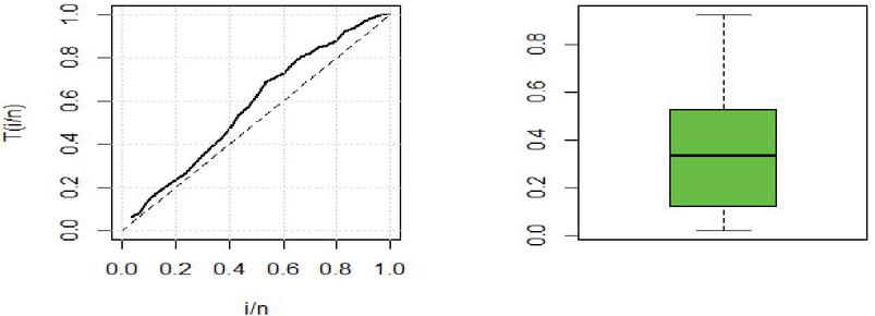
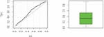
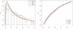
Figure 3 TTT and box plot for data set I.

The OFrPFD is fitted to the given dataset and compared on the basis of following statistics: maximum log-likelihood, Akaike Information Criterion (AIC), Bayesian Information Criterion (BIC) criteria. The nonparametric test, Anderson–Darling (A*), Cramer–von Mises (W*), and Kolmogorov Smirnov (KS) are applied to measure the closeness between the empirical and fitted distributions. Further, to illustrate the shape of data sets, we present a two approaches which are based on graphs i.e., total time test transform (TTT) plot and box plot.

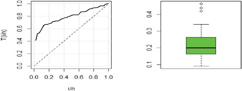
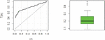
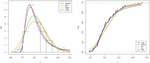
Figure 4 TTT and box plot for data set II.

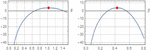
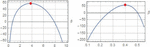
Figures 3–4 show TTT plot and box plot for both data sets. Tables 8 and 9 give the MLEs and their standard errors (S.E.) given in parentheses and the values of the four accuracy measures for the fitted models including OFrPFD and other competitive distributions to the data sets I and II, respectively. Table 10 gives the confidence interval of parameters for both 95% and 99% levels for both data sets. Empirical data is plotted along with fitted densities for both data sets in Figures 5–6. To illustrate the likelihood equations, we plot the profile of the log-likelihood of $\mathrm{\Phi }=(\theta ,\beta )$ in Figures 7–8. We also use some estimation methods discussed in Section 4 to estimate the unknown parameters from both data sets. The point estimates of the OFrPF parameters are obtained using the given six methods and the KS and P-values are computed in Table 11.

Table 8 MLEs and goodness-of-fit measures for Tensile Strength data

Model	MLEs	LogLik	AIC	BIC	A	W	KS
OFrPF	$\widehat{\theta }=1.0204$ $\widehat{\beta }=0.4269$	3.9557	$-$3.9115	$-$1.1091	0.1229	0.0206	0.0538
Beta	$\widehat{\theta }=0.9667$ $\widehat{\beta }=1.6205$	3.3051	$-$2.6101	0.1923	0.1703	0.0321	0.0669
Kw	$\widehat{\theta }=0.9627$ $\widehat{\beta }=1.6084$	3.3110	$-$2.6221	0.1803	0.1633	0.0307	0.0750
UGD	$\widehat{\theta }=1.0436$ $\widehat{\beta }=0.4198$	3.9088	$-$3.8576	$-$1.0552	0.1299	0.0354	0.0629

Table 9 MLEs and goodness-of-fit measures for Data II.

Model	MLEs	LogLik	AIC	BIC	A	W	KS
OFrPF	$\widehat{\theta }=3.7469$ $\widehat{\beta }=0.3992$	58.216	$-$112.43	$-$108.69	0.1882	0.0258	0.0733
Beta	$\widehat{\theta }=5.9415$ $\widehat{\beta }=21.206$	55.600	$-$107.20	$-$103.46	0.7767	0.1300	0.1427
Kw	$\widehat{\theta }=2.7186$ $\widehat{\beta }=44.652$	52.492	$-$100.98	0$-$97.24	1.2892	0.2060	0.1533
UGD	$\widehat{\theta }=0.0053$ $\widehat{\beta }=2.9893$	56.644	$-$109.29	$-$105.55	0.3574	0.0433	0.0808

Table 10 Confidence intervals for parameters of OFrPF distribution

	CI	$\theta$	$\beta$
Data I	95%	$[0.7069,1.3340]$	$[0.3207,0.5332]$
	99%	$[0.6085,1.4323]$	$[0.2873,0.5666]$
	CI	$\theta$	$\beta$
Data II	95%	$[2.9161,4.5774]$	$[0.3764,0.4220]$
	99%	$[2.6551,4.8384]$	$[0.3693,0.4292]$

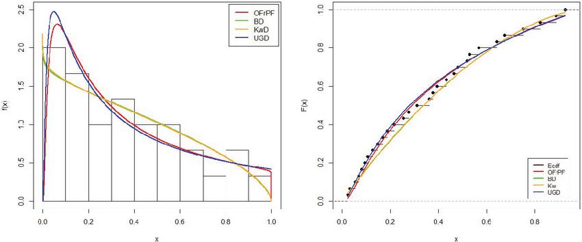
Figure 5 Fitted pdf and cdf for the data I.

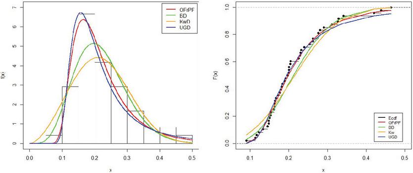
Figure 6 Fitted pdf and cdf for the data II.

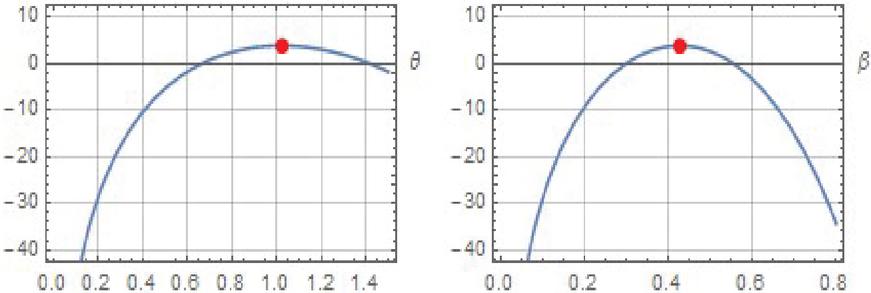
Figure 7 The curves log-likelihood function of parameters data set I.

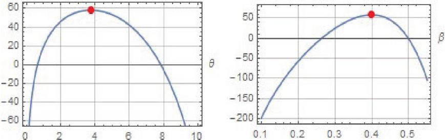
Figure 8 The curves log-likelihood function of parameters data set II.

Table 11 The parameter estimates of OFrPF distribution under different estimation methods for data sets

	Data Set I			Data Set II
Method	$\widehat{\theta }$	$\widehat{\beta }$	K-S (P-value)	$\widehat{\theta }$	$\widehat{\beta }$	K-S (P-value)
MLE	1.0204	0.4269	0.9727	3.7469	0.3992	0.9596
OLS	0.9240	0.4314	0.9891	3.8186	0.3998	0.9612
WLS	0.9289	0.4270	0.9983	3.7636	0.4002	0.9401
ADE	0.9781	0.4322	0.9995	3.8358	0.4003	0.9739
CVM	0.9660	0.4366	0.9987	3.9413	0.4005	0.9690
Percentile	0.9776	0.4407	0.9691	3.5965	0.3985	0.9341

From Tables 8 and 9, it is found that the OFrPF distribution has the largest Log-likelihood value and the smallest AIC, BIC, A, W, and K-S values than other models’ measures. It is shown that the OFrPF performs better than other fitted models to both data sets because it has larger p-values. According to Figures 5–6, the closeness of the fitted PDF and CDF using the OFrPF distribution to the empirical PDF and CDF is clear. Thus, the OFrPF distribution fits both data sets better than other models. Also the model parameters are estimated using six different estimation methods discussed in Section 4, the estimates are presented in Table 11. And on the basis of observation from Table 11, we can conclude that the ADE method provides better estimates the OFrPF parameters for both data sets. Overall, all the estimation methods perform well for both data sets.

9 Conclusion

This article introduces a new odd Fréchet power (OFrPF) distribution. Numerous properties of OFrPF distribution are obtained. Reliability analysis is carried out for proposed distribution. The parameters of the OFrPF distribution are estimated using different methods; maximum likelihood, least squares, weighted least squares, percentile, Cramer-von Mises, Anderson-Darling. A simulation study is conducted for evaluation performances of estimators of OFrPF distribution under different estimation methods. The application of OFrPF distribution is given for two real data sets under derived estimation methods. From the comparisons of the proposed distribution with other existing unit models, we conclude that the proposed distribution performs better in fitting and estimation than the existing distributions.

The present study can be extended for statistical inferences using Bayesian analysis and different sampling plans (i.e., Rank Set Sampling (RSS)) scheme can be considered. The reliability analysis, for example, stress strength reliability estimation using simple random sampling and RSS can also considered.

Acknowledgment

We are thankful to the editor and reviewers for their valuable suggestions to improve the quality of the paper.

References

Aarset, M.V., How to identify a bathtub hazard rate. IEEE Transactions on Reliability, 1987. 36(1): p. 106–108.

Bourguignon, M., Silva, R. B., and Cordeiro, G. M. (2014). The Weibull-G Family of Probability Distributions. 12, 53–68.

Cook, D. O., Kieschnick, R., and McCullough, B. D. (2008). Regression analysis of proportions in finance with self selection. Journal of Empirical Finance, 15(5), 860–867.

Cordeiro, G. M., Alizadeh, M., Ozel, G., Hosseini, B., Moises, E., Ortega, M., and Altun, E. (2016). The generalized odd log-logistic family of distributions: properties, regression models and applications. Journal of Statistical Computation and Simulation, 0(0), 1–25. https://doi.org/10.1080/00949655.2016.1238088

Cordeiro, G. M., and dos Santos Brito, R. (2012). The beta power distribution. Brazilian Journal of Probability and Statistics, 26(1), 88–112. https://doi.org/10.1214/10-BJPS124

Cribari-Neto, F., and Souza, T. C. (2013). Religious belief and intelligence: Worldwide evidence. Intelligence, 41(5), 482–489.

Dallas, A. C. (1976). Characterizing the Pareto and power distributions. Annals of the Institute of Statistical Mathematics, 28(1), 491–497.

Gupta, A. K., and Nadarajah, S. (2004). Handbook of beta distribution and its applications. CRC press.

Haq, M. A., and Elgarhy, M. (2018). The odd Fréchet-G family of probability distributions. Journal of Statistics Applications & Probability, 7(1), 189–203.

Haq, M. A., Hashmi, S., Aidi, K., Ramos, P. L., and Louzada, F. (2020). Unit Modified Burr-III Distribution: Estimation, Characterizations and Validation Test. Annals of Data Science. https://doi.org/10.1007/s40745-020-00298-6

Haq, M. A. ul, Elgarhy, M., and Hashmi, S. (2019). The generalized odd Burr III family of distributions: properties, applications and characterizations. Journal of Taibah University for Science, 13(1), 961–971. https://doi.org/10.1080/16583655.2019.1666785

Haq, M. A., Butt, N. S., Usman, R. M., and Fattah, A. A. (2016). Transmuted power function distribution. Gazi University Journal of Science, 29(1), 177–185.

Haq, M. A., Usman, R. M., Bursa, N., and Özel, G. (2018). McDonald power function distribution with theory and applications.

Hassan, A. S., and Assar, S. M. (2017). The exponentiated Weibull power function distribution. Journal of Data Science, 16(2), 589–614.

Johnson, N. L. (1949). Systems of frequency curves generated by methods of translation. Biometrika, 36(1/2), 149–176.

Kumaraswamy, P. (1980). A generalized probability density function for double-bounded random processes. Journal of Hydrology, 46(1–2), 79–88.

Lehmann, E. L., and Casella, G. (2006). Theory of point estimation. Springer Science & Business Media.

Mazucheli, J, Menezes, A. F. B., and Ghitany, M. E. (2018). The unit-Weibull distribution and associated inference. J. Appl. Probab. Stat, 13, 1–22.

Mazucheli, Josmar, Menezes, A. F. B., and Chakraborty, S. (2018). On the one parameter unit-Lindley distribution and its associated regression model for proportion data. Journal of Applied Statistics, 4763. https://doi.org/10.1080/02664763.2018.1511774

Quesenberry, C. P., and Hales, C. (1980). Concentration bands for uniformity plots. Journal of Statistical Computation and Simulation, 11(1), 41–53.

Tahir, M. H., Alizadeh, M., Mansoor, M., and Cordeiro, G. M. (2016). The Weibull-power function distribution with applications. 45(1), 245–265.

Topp, C. W., and Leone, F. C. (1955). A family of J-shaped frequency functions. Journal of the American Statistical Association, 50(269), 209–219.

Usman, R. M., Haq, M. A., Bursa, N., Özel, G., & Info, A. (2018). Exponentiated Transmuted Power Function Distribution: Theory & Applications. June. http://dergipark.gov.tr/gujs

Biographies

Muhammad Ahsan ul Haq received his MPhil degree in Statistics from the College of Statistical and Actuarial Sciences, University of the Punjab, Lahore, Pakistan. Also, he is a PhD Research Scholar at University of the Punjab, Pakistan. He is doing PhD Under the supervision of Dr. Ahmed Zogo Memon and Dr. Sohail Chand. His research interests include Mathematical and Applied Statistics, Distribution Theory, reliability analysis, and mixture distributions.

Mohammed Albassam received his B.Sc. degree from Mathematics department at King Abdulaziz University in 1990, M.Sc. and Ph.D. degrees from School of Mathematics and Statistics at University of Sheffield, UK, in 1995 and 2000. He is currently working as an Associate Professor at Statistics department in King Abdulaziz University. He has published many articles in International journals. His fields of interest are Statistical inference, Distributions theory, Neutrosophic Statistics and Time series Analysis.

Muhammad Aslam did his M.Sc in Statistics (2004) from GC University Lahore with Chief Minister of the Punjab merit scholarship, M. Phil in Statistics (2006) from GC University Lahore with the Governor of the Punjab merit scholarship, and Ph.D. in Statistics (2010) from National College of Business Administration & Economics Lahore under the kind supervision of Prof. Dr. Munir Ahmad. He worked as a lecturer of Statistics in Edge College System International from 2003–2006. He also worked as a Research Assistant in the Department of Statistics, GC University Lahore from 2006 to 2008. Then he joined the Forman Christian College University as a lecturer in August 2009. He was a part of visiting faculty member, Department of Statistics, GC University Lahore from 2009 to 2014. He worked as Assistant Professor in the same University from June 2010 to April 2012. He worked in the same department as Associate Professor from June 2012 to October 2014. He worked as Associate Professor of Statistics in the Department of Statistics, Faculty of Science, King Abdulaziz University, Jeddah, Saudi Arabia from October 2014 to March 2017. He taught summer courses as Visiting Faculty of Statistics at Beijing Jiaotong University, China in 2016. Currently, he is working as a Full Professor of Statistics in the department of Statistics, King Abdul-Aziz University Jeddah, and Saudi Arabia. He has published more than 437 research papers in national and international well-reputed journals including, for example, IEEE Access, Journal of Applied Statistics, European Journal of Operation Research, Information Sciences, Journal of Process Control, Journal of the Operational Research Society, Applied Mathematical Modeling, International Journal of Fuzzy Systems, Complexity, ACS Ogema, Symmetry, International Journal of Advanced Manufacturer Technology, Communications in Statistics, Journal of Testing and Evaluation and Pakistan Journal of Statistics etc. His papers have been cited more than 4400 times with h-index 33 and i-10 index 114 (Google Scholar). His papers have been cited more than 2700 times with h-index 25 (Web of Science Citations). He is the author of three books published by VDM, Germany, Springer and Wiley, respectively. He has published 10 chapters in well-reputed books. He is also HEC approved PhD supervisor since 2011. He supervised 5 PhD theses, more than 25 M.Phil theses and 3 M.Sc. theses. Dr. Muhammad Aslam is currently supervising 2 Master theses in Statistics. He is a reviewer of more than 70 well-reputed international journals. He has reviewed more than 160 research papers for various well-reputed international journals. He received meritorious services award in research from National College of Business Administration & Economics Lahore in 2011. He received Research Productivity Award for the year 2012 by Pakistan Council for Science and Technology. His name Listed at 2nd Position among Statistician in the Directory of Productivity Scientists of Pakistan 2013. His name Listed at 1st Position among Statistician in the Directory of Productivity Scientists of Pakistan 2014. He got 371 positions in the list of top 2210 profiles of Scientist of Saudi Institutions 2016. He Received King Abdulaziz University Excellence Awards in Scientific Research for the paper entitled “Aslam, M., Azam, M., Khan, N. and Jun, C.-H. (2015). A New Mixed Control Chart to Monitor the Process, International Journal of Production Research, 53 (15), 4684–4693. He Received King Abdulaziz University citation award for the paper entitled “Azam, M., Aslam, M. and Jun, C.-H. (2015). Designing of a hybrid exponentially weighted moving average control chart using repetitive sampling, International Journal of Advanced Manufacturing Technology, 77:1927–1933 in 2018. Prof. Muhammad Aslam is listed in, top 2% of scientists of the world in the list released by Stanford University, USA. He is at rank 35/93 among the King Abdulaziz University Scientist.

Prof. Muhammad Aslam introduced the area of Neutrosophic Statistical Quality Control (NSQC) the first time. He is the founder of neutrosophic inferential statistics (NIS) and NSQC. His contribution is the development of neutrosophic statistics theory for the inspection, inference, and process control. He originally developed the theory in these areas under the Neutrosophic Statistics. He extended the Classical Statistics theory to Neutrosophic Statistics originally in 2018.

He is the member of the editorial board of Electronic Journal of Applied Statistical Analysis, Neutrosophic Sets and Systems, Pakistan Journal of Commence and Social sciences and International Journal of Neutrosophic Science. He is also a member of the Islamic Countries Society of Statistical Sciences. He is appointed as an external examiner for 2016/2017–2018/2019 triennium at The University of Dodoma, Tanzania. His areas of interest include Industrial Statistics, neutrosophic inferential statistics, neutrosophic statistics, neutrosophic quality control, neutrosophic applied statistics, and classical applied Statistics.

Sharqa Hashmi completed her PhD from University of the Punjab, Pakistan. She did her research work under the supervisor is Prof. Dr. Ahmed Zogo Memon. She got first position (Gold Medal) in the M.Sc (Statistics) in 1996 from University of the Punjab, Pakistan. She received her B.Sc. in Statistics from the same University. Her research interests include mathematical statistics, probability distributions, and distribution theory. She worked as a lecturer in department of statistics, Lahore College for Women University (LCWU), Lahore, Pakistan from 1999 to 2011. She has been working an Assistant Professor of Statistics in same university since 2011. She also won foreign PhD Scholarship under faculty development program of LCWU, in 2007 and got admission in UK and Australia but unable to join due to some family issues.

She conducted a five day workshop as resource person titled “Data Visualization and Optimization of Generalized Models through Mathematica” from 24${}^{\mathrm{th}}$ Feb, 2020 to 28${}^{\mathrm{th}}$ Feb., 2020 at LCWU, Lahore, Pakistan. She also conducted a two day workshop as resource person titled “Statistical tools in Pharmacy” from 20–21 Feb, 2020. She worked as Technical Advisor in six days workshop titled “TIDYVERSE FOR DATA SCIENCE” from 15${}^{\mathrm{th}}$ July, 2019 to 20${}^{\mathrm{th}}$ July, 2019 at Bureau of Statistics, Lahore. Also worked as Co-instructor in six days workshop titled “TIDYVERSE FOR DATA SCIENCE” from 29${}^{\mathrm{th}}$ July, 2019 to 3rd August, 2019 at Bureau of Statistics, Lahore and many online workshops during COVID.19.

Journal of Reliability and Statistical Studies, Vol. 14, Issue 1 (2021), 141–172.
doi: 10.13052/jrss0974-8024.1417
© 2021 River Publishers