The Beta Reduced Modified Weibull Distribution with Applications to Reliability Data

Lazhar Benkhelifa

Department of Mathematics and Informatics, Larbi Ben M’Hidi University, Oum El Bouaghi, 04000, Algeria

E-mail: l.benkhelifa@yahoo.fr

Received 31 October 2020; Accepted 27 March 2021; Publication 22 June 2021

Abstract

In this paper, we introduce a new probability distribution with application in reliability called the beta reduced modified Weibull distribution. The proposed distribution presents a more flexible model and has the capability to capture decreasing, increasing, bathtub, unimodal (upside-down bathtub) and modified unimodal shaped hazard rates. Also, this distribution has a bathtub-shaped hazard rate function with a long useful life period, which is desirable property in reliability analysis. We obtain the expansions for the moments, quantile function, stress-strength reliability, density function of the order statistics and their moments. We use the method of maximum likelihood to estimate the model parameters for complete and right-censored data. We evaluate the performance of the maximum likelihood estimators in a simulation study. We analyze three reliability data sets, complete and censored, to examine the flexibility of the proposed model.

Keywords: Beta distribution, Hazard rate function, Modified Weibull distribution, Maximum likelihood estimation.

1 Introduction

Among the parametric probability distributions, the Weibull distribution is the most widely applied model in reliability analysis such as reliability engineering, decision-making reliability and firmware reliability. Since the Weibull distribution is only applicable for modeling the data with increasing, decreasing or constant hazard rate, its applicability may be restricted to the data that have non-monotone hazard rate shapes such as the bathtub shape, unimodal (upside-down bathtub) or modified unimodal shape. For this reason, several authors have proposed various modifications and generalizations of the Weibull distribution in the last few decades. For example, Lai et al. [1] proposed a three-parameter modified Weibull with a bathtub-shaped hazard rate function. Bebbington et al. [2] proposed a two-parameter flexible Weibull extension with monotone and bathtub-shaped hazard rate functions. Sarhan and Apaloo [3] proposed the four-parameter exponentiated modified Weibull extension distribution which exhibits a bathtub-shaped hazard rate function. Famoye et al. [4] proposed the four-parameter beta Weibull distribution with unimodal, increasing, decreasing and bathtub-shaped hazard rate functions. Benkhelifa [5] introduced the Weibull Birnbaum-Saunders distribution with four parameters.

According to Nelson [6], the distributions which provide more flexible distributions usually require at least five parameters. Among the five parameters modified Weibull distributions we mention, the beta modified Weibull distribution [7], the McDonald Weibull distribution [8], the beta generalized Weibull distribution [9], the beta Sarhan-Zaindin modified Weibull distribution [10], the additive modified Weibull distribution [11], the new generalized odd log-logistic flexible Weibull distribution [12] and the exponentiated additive Weibull distribution [13]. All theses distributions have monotone, bathtub-shaped and unimodal hazard rate functions. Almalki and Yuan [14] introduced a new modified Weibull with five parameters and its hazard rate function can be increasing, decreasing or bathtub-shaped. The cumulative distribution function (cdf) of this distribution is

$G_{MW}(x)=1-e^{-\alpha x^{\theta }-\beta x^{\gamma }{e}^{\lambda x}},$

(1)

where $\alpha ,\beta >0$ are scale parameters, $\theta ,\gamma >0$ are shape parameters and $\lambda >0$ is an acceleration parameter. In order to avoid some estimation problems, Almalki [15] proposed a reduced version, with three parameters, of the Almalki-Yuan modified Weibull distribution. The cdf of the reduced modified Weibull (RMW) distribution is obtained by setting $\gamma =\theta =1/2$ in (1) as follows

$G(x)=1-e^{-\alpha \sqrt{x}-\beta \sqrt{x}{e}^{\lambda x}},$

(2)

The probability density function (pdf) of the RMW distribution is

$g(x)={\displaystyle \frac{1}{2\sqrt{x}}}[\alpha +\beta e^{\lambda x}(1+2\lambda x)]e^{-\alpha \sqrt{x}-\beta \sqrt{x}{e}^{\lambda x}}.$

The RMW distribution can exhibit bathtub-shaped hazard rate function. Some real data, particularly in reliability engineering, have a bathtub-shaped hazard rate functions with a long useful life period with constant hazard rate in the middle. For example, electric machine life cycles and electronic devices (see [16]). The RMW distribution has this property. The beta-G family of distributions introduced by Eugene et al. [17] is one of the methods that make the distributions richer and flexible to model the real life data by adding two shapes parameters. The hazard rate function of the RMW distribution can exhibit bathtub shapes but not more other complicated shapes. For this reason, in this paper, we introduce a new five-parameter that generalizes the RMW distribution by using the beta-G family of distributions. The proposed distribution will be called the beta reduced modified Weibull (BRMW) distribution. The BRMW model provides a better fit than the RMW distribution and its hazard rate can be monotone, bathtub-shaped and unimodal failure rate. It can also have a bathtub-shaped hazard rate function with a long flat useful life period. The rest of the paper is organized as follows. In Section 2, we define the BRMW model. In Sections 3, 4, 5 and 6 we give the expansions for the $r$th moment of the BRMW distribution, the quantile function, the stress-strength reliability and the order statistics, respectively. In Section 7, we discuss maximum likelihood estimation of the model parameters for complete and right-censored data. In Section 8, we conduct a simulation study to check the performance of the maximum likelihood estimates. In Section 9, we analyze three reliability data sets, complete and right-censored, to demonstrate the usefulness of the new model. In Section 10, we give some concluding remarks.

2 Beta Reduced Modified Weibull Distribution

In order to obtain greater flexibility in modeling real data sets, Eugene et al. [17] introduced the beta-generated family of distributions by using the beta random variable. For an arbitrary parent or baseline cdf $G(x)$, the cdf of the beta generalized family is given by

$$F(x)=I_{G(x)}(a,b)=\frac{1}{B(a,b)}{\int }_0^{G(x)}{t}^{a-1}{(1-t)}^{b-1}\mathit{d}t,$$

(3)

where $a>0$ and $b>0$ are two shape parameters, $I_y(a,b)=B_y(a,b)$/ $B(a,b)$ is the incomplete beta function ratio, $B_y(a,b)={\int }_0^y{t}^{a-1}{(1-t)}^{b-1}\mathit{d}t$ is the incomplete beta function, $B(a,b)=\mathrm{\Gamma }(a)\mathrm{\Gamma }(b)/\mathrm{\Gamma }(a+b)$ is the complete beta function and $\mathrm{\Gamma }(.)$ is the gamma function. The pdf corresponding to (3) is

$$f(x)=\frac{g(x)}{B(a,b)}{[G(x)]}^{a-1}{[1-G(x)]}^{b-1},$$

where $g(x)=dG(x)/dx$ is the baseline pdf. By substituting (2) in (3), the cdf of the BRMW distribution with five parameters ($\alpha ,\beta >0,\lambda >0,a>0$ and $b>0$) can be defined by

$$\begin{array}{cc}\hfill F(x)& =I_{1-e^{-\alpha \sqrt{x}-\beta \sqrt{x}{e}^{\lambda x}}}(a,b)\hfill \\ & =\frac{1}{B(a,b)}{\int }_0^{1-e^{-\alpha \sqrt{x}-\beta \sqrt{x}{e}^{\lambda x}}}{t}^{a-1}{(1-t)}^{b-1}\mathit{d}t.\hfill \end{array}$$

The pdf of the BRMW distribution is given by

$$f(x)=\frac{[\alpha +\beta e^{\lambda x}(1+2\lambda x)]{(1-e^{-\alpha \sqrt{x}-\beta \sqrt{x}{e}^{\lambda x}})}^{a-1}{e}^{-\alpha b\sqrt{x}-\beta b\sqrt{x}{e}^{\lambda x}}}{2\sqrt{x}B(a,b)}.$$

(4)

The BRMW distribution includes as special cases the RMW distribution and the exponentiated RMW (ERMW) distribution. For $a=b=1$, we obtain the RMW distribution. When $b=1$, the BRMW distribution is reduced to ERMW distribution.

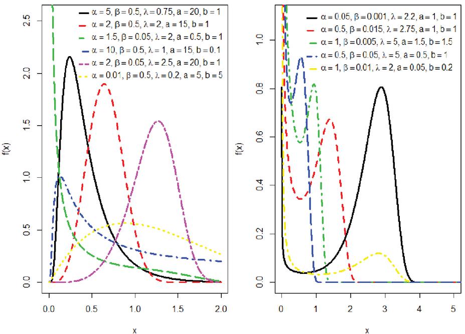
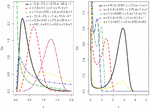
Figure 1 shows some possible shapes of the pdf (4) for some parameter values of $\alpha ,\beta >0,\lambda >0,a>0$ and $b>0$. Then, we observe that the pdf (4) can take various forms depending on the parameter values. It is evident that the BRMW distribution is much more flexible than the RMW and the ERMW distributions.

The hazard function of the BRMW distribution is given by

$$h(x)=\frac{[\alpha +\beta e^{\lambda x}(1+2\lambda x)]{(1-e^{-\alpha \sqrt{x}-\beta \sqrt{x}{e}^{\lambda x}})}^{a-1}{e}^{-\alpha b\sqrt{x}-\beta b\sqrt{x}{e}^{\lambda x}}}{2\sqrt{x}B(a,b)(1-I_{1-e^{-\alpha \sqrt{x}-\beta \sqrt{x}{e}^{\lambda x}}}(a,b))}.$$

Figure 1 Plots of the pdf of the BRMW distribution for some parameter values.

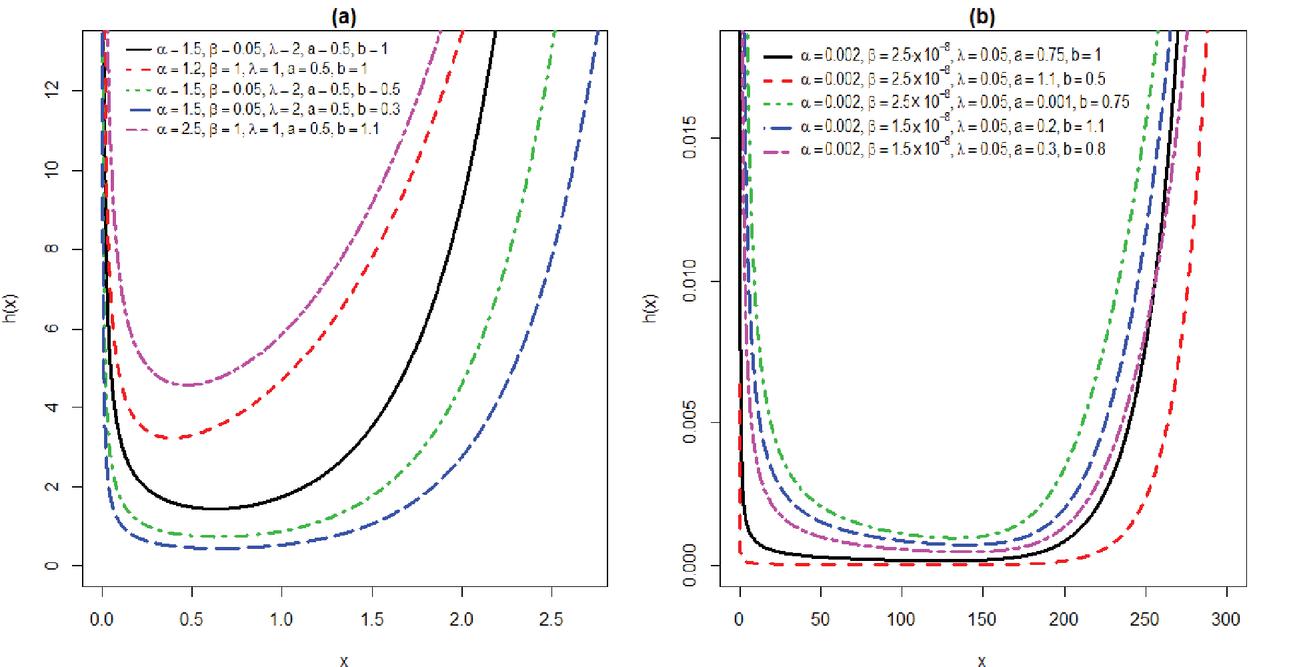
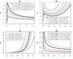
Figure 2 (a) Bathtub-shaped hazard rate functions. (b) Bathtub-shaped hazard rate functions with long useful life period.

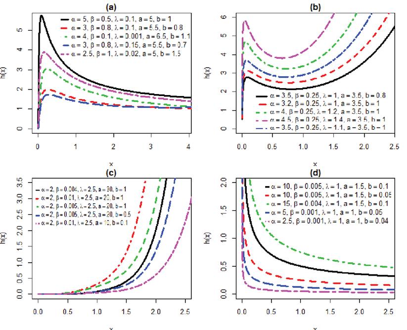
In Figures 2 and 3, we plot the hazard rate function of the BRMW distribution for selected values of $\alpha ,\beta >0,\lambda >0,a>0$ and $b>0$. We observe, in Figure 3, that the hazard rate function of the BRMW distribution can be decreasing, increasing, bathtub, unimodal (upside-down bathtub) and modified unimodal shaped hazard rates. The BRMW distribution can also have a bathtub-shaped hazard rate function with a long useful life period (Figure 2). Therefore, the BRMW distribution is quite flexible and can be used to fit various kinds of data sets in reliability analysis.

Figure 3 Plots of the hazard rate function of the BRMW distribution for some parameter values. (a) Upside-down bathtub hazard rate functions. (b) Modified unimodal shaped hazard rate functions. (c) Increasing hazard rate functions. (d) Decreasing hazard rate functions.

3 General Formula for the Moments

In this section, we derive the expression for $r$th order moment of BRMW distribution. It allows us to determine the expected life time of a device, dispersion, skewness and kurtosis in reliability data sets. The $r$th moment of the BRMW distribution is defined by

$$E(X^r)={\int }_0^{\mathrm{\infty }}{x}^{r}f(x)\mathit{d}x,$$

where $f(x)$ is defined in (4). The moments can be obtained via an algebraic expansion which is more efficient than computing those directly by numerical integration of its density function. Then, using the binomial series expansion, for $|z|<1,\eta >0,$

$${(1-z)}^{\eta -1}=\sum _{k=0}^{\mathrm{\infty }}\frac{{(-1)}^k\mathrm{\Gamma }(\eta )}{\mathrm{\Gamma }(\eta -k)}{z}^k,$$

(5)

we obtain

$${(1-e^{-\alpha \sqrt{x}-\beta \sqrt{x}{e}^{\lambda x}})}^{a-1}=\sum _{k=0}^{\mathrm{\infty }}\frac{{(-1)}^k\mathrm{\Gamma }(\eta )}{\mathrm{\Gamma }(\eta -k)}{e}^{-k(\alpha \sqrt{x}-\beta \sqrt{x}{e}^{\lambda x})}.$$

(6)

Substituting (6) in (4), we get

$$f(x)=\sum _{k=0}^{\mathrm{\infty }}\frac{{(-1)}^k\mathrm{\Gamma }(a+b)}{(b+k)\mathrm{\Gamma }(a-k)\mathrm{\Gamma }(b)}g(x;(b+k)\alpha ,(b+k)\beta ,a,b),$$

(7)

where $g(x;(b+k)\alpha ,(b+k)\beta ,a,b)$ is the pdf of the RMW distribution with parameters $(b+k)\alpha ,(b+k)\beta ,a$ and $b$. Therefore,

$$E(X^r)=\frac{\mathrm{\Gamma }(a+b)}{\mathrm{\Gamma }(b)}\sum _{k=0}^{\mathrm{\infty }}\frac{{(-1)}^k}{(b+k)\mathrm{\Gamma }(a-k)}E(Y^r),$$

(8)

where $E(Y^r)$ is the $r$th moment of a random variable $Y$ having the RMW distribution with parameters $(b+k)\alpha ,(b+k)\beta ,a$ and $b$. Then, from Equation (5) in Almalki [15], we can get

$$E(Y^r)=2r\sum _{n,m=0}^{\mathrm{\infty }}\frac{{(-b\beta -k\beta )}^n{(n\lambda )}^m\mathrm{\Gamma }(n+2(m+r))}{n!m!{(b\alpha +k\alpha )}^{n+2(m+r)}}.$$

(9)

Substituting (9) in (8), we obtain

$$E(Y^r)=2r\sum _{k,n,m=0}^{\mathrm{\infty }}\frac{{(-1)}^{k+n}{(b\beta +k\beta )}^n{(n\lambda )}^m\mathrm{\Gamma }(n+2(m+r))\mathrm{\Gamma }(a+b)}{(b+k)\mathrm{\Gamma }(a-k)n!m!{(b\alpha +k\alpha )}^{n+2(m+r)}\mathrm{\Gamma }(b)}.$$

To describe any data, we can use the first four moments. The first moment or the mean is a measure of the center of the distribution. The second moment about the mean is equal to the variance which measures the spread of the distribution about the mean. The skewness measures the symmetry of a distribution whereas the kurtosis measures the peakedness of a distribution. We give the values of the first four moments, variance, skewness and kurtosis of the BRMW distribution for some selected values of the parameters in Table 1. The R code to compute the moments is provided in Appendix. (R is a free software environment for statistical computing and graphics).

Table 1 First four moments, variance, skewness and kurtosisof the BRMW distribution for some parameter values: $\alpha =2.5$ $\beta =1.25$ and $\lambda =0.5$

	$a=0.5$,	$a=0.5$,	$a=1.5$,	$a=5.5$,	a=5.5,	$a=5$
	$b=2$	$b=4$	$b=1.5$	$b=2.5$	$b=10$	$b=3$
$E(X)$	0.015695	0.003697	0.084153	0.135653	0.017375	0.097167
$E(X^2)$	0.002356	0.00015	0.02481	0.032344	0.000538	0.017368
$E(X^3)$	0.000795	$1.6\times {10}^{-5}$	0.013273	0.011577	$2.6\times {10}^{-5}$	0.004804
$E(X^4)$	0.00042	$3.0\times {10}^{-6}$	0.010101	0.005614	$2\times {10}^{-6}$	0.001844
Variance	0.00211	0.000137	0.017729	0.013943	0.000236	0.007927
Skewness	7.133163	8.981911	3.474405	2.068941	2.307967	2.233645
Kurtosis	80.85056	146.0047	17.79799	6.708253	9.273554	8.024071

4 Quantile Function

The quantile function of the BRMW distribution can be obtained by inverting the following equation:

$$I_{1-e^{-\alpha \sqrt{x}-\beta \sqrt{x}{e}^{\lambda x}}}(a,b)=u,0\le u\le 1,$$

i.e.,

$$1-e^{-\alpha \sqrt{x}-\beta \sqrt{x}{e}^{\lambda x}}=I_u^{-1}(a,b),$$

where $I_u^{-1}(a,b)$ denotes the inverse of the incomplete beta function with parameters a and b. Therefore, we obtain the quantile function of the BRMW distribution by solving the following equation:

$$\alpha \sqrt{x}-\beta \sqrt{x}{e}^{\lambda x}+\log (1-I_u^{-1}(a,b))=0.$$

It is clear that this equation does not have a closed form solution in $x$, and hence we use numerical methods to obtain the quantile function of the BRMW distribution.

To generate random variables from BRMW distribution, we have the following algorithm:

• Set the values of parameters: $\alpha ,\beta >0,\lambda >0,a>0$ and $b>0$.

• Generate $V_i$ from beta distribution with parameters $a$ and $b$, for $i=1,\mathrm{\dots },n$.

• Solve the following equation for $x_i$:

$$\alpha \sqrt{x_i}-\beta \sqrt{x_i}{e}^{\lambda x_i}+\log (1-V_i)=0.$$

In the Appendix, we give the R code to generate random variables from BRMW distribution.

5 Order Statistics

The order statistics play an important role in reliability analysis. In this section, we give the pdf of the order statistic $X_{i,n}$, and its $p$th moment, for the BRMW distribution. If $X_1,\mathrm{\dots },X_n$ is a random sample from the BRMW distribution, and $X_{1,n},\mathrm{\dots },X_{n,n}$ are the order statistics from this sample, then, from Arnold et al. [18], the pdf of $X_{i,n}$ is given by

$f_{i,n}(x)={\displaystyle \frac{f(x){[F(x)]}^{i-1}{[1-F(x)]}^{n-i}}{B(i,n-i+1)}},i=1,\mathrm{\dots },n.$

Now, we derive an expansion for $f_{i,n}(x)$. Using the binomial series expansion of ${[1-F(x)]}^{n-i}$, we obtain

${[1-F(x)]}^{n-i}={\displaystyle \sum _{l=0}^{n-i}}{\displaystyle \frac{{(-1)}^l\mathrm{\Gamma }(n)}{\mathrm{\Gamma }(n-l)}}{[F(x)]}^l,$

then

$f_{i,n}(x)={\displaystyle \frac{f(x)}{B(i,n-i+1)}}{\displaystyle \sum _{l=0}^{n-i}}{\displaystyle \frac{{(-1)}^l\mathrm{\Gamma }(n)}{\mathrm{\Gamma }(n-l)}}{[F(x)]}^{l+i-1}.$

(10)

The incomplete beta function expansion for $b$ real non-integer gives

$F(x)=I_{G(x)}(a,b)={\displaystyle \sum _{k=0}^{\mathrm{\infty }}}{t}_k{[G(x)]}^{k+a},$

where

$t_k={\displaystyle \frac{\mathrm{\Gamma }(1-b+k)}{k!(a+k)B(a,b)\mathrm{\Gamma }(1-b)}}.$

From Gradshteyn and Ryzhik [19] (Section 0.314), for a power series raised to a positive integer s, we have

${\left({\displaystyle \sum _{j=0}^{\mathrm{\infty }}}{a}_j{u}^j\right)}^s={\displaystyle \sum _{j=0}^{\mathrm{\infty }}}{d}_{s,j}{u}^j,$

(11)

where the coefficients $d_{s,j}$ (for $j=1,2,\mathrm{\dots }$) are determined from the recurrence equation

$d_{s,j}={(j{a}_0)}^{-1}{\displaystyle \sum _{m=1}^j}[m(s+1)-j]a_m{d}_{s,j-m},$

(12)

with $d_{s,0}=a_0^s$. Then, by using (11) and after some simplifications, we get

${\left({\displaystyle \sum _{k=0}^{\mathrm{\infty }}}{t}_k{[G(x)]}^{k+a}\right)}^{i+l-1}={\displaystyle \sum _{k=0}^{\mathrm{\infty }}}{t}_{i+l-1,k}{(1-e^{-\alpha \sqrt{x}-\beta \sqrt{x}{e}^{\lambda x}})}^{k+a(i+l-1)},$ (11)

where the coefficients $t_{i+l-1,k}$ follow from Equation (12). Substituting (4) and (13) in (10), we obtain

$f_{i,n}(x)={\displaystyle \frac{1}{B(i,n-i+1)}}$	${\displaystyle \sum _{l=0}^{n-i}}{\displaystyle \frac{{(-1)}^l\mathrm{\Gamma }(n)}{\mathrm{\Gamma }(n-l)}}{\displaystyle \sum _{k=0}^{\mathrm{\infty }}}{t}_{i+l-1,k}{\displaystyle \frac{[\alpha +\beta (1+2\lambda x)e^{\lambda x}]}{2\sqrt{x}B(a,b)}}$
	$\times e^{-\alpha \sqrt{x}-\beta \sqrt{x}{e}^{\lambda x}}{(1-e^{-\alpha \sqrt{x}-\beta \sqrt{x}{e}^{\lambda x}})}^{k+a(i+l-1)}.$

Using the binomial series expansion of ${[1-e^{-\alpha \sqrt{x}-\beta \sqrt{x}{e}^{\lambda x}}]}^{k+a(i+l)-1}$, we obtain

$f_{i,n}(x)={\displaystyle \sum _{k,r=0}^{\mathrm{\infty }}}{v}_{i,k,r}g(x;(r+b)\alpha ,(r+b)\beta ,a,b),$

(14)

where

$v_{i,k,r}={\displaystyle \frac{{(-1)}^r\mathrm{\Gamma }(n)}{(r+b)B(a,b)B(i,n-i+1)}}{\displaystyle \sum _{l=0}^{n-i}}{\displaystyle \frac{{(-1)}^l{t}_{i+l-1,k}\mathrm{\Gamma }(k+a(i+l))}{\mathrm{\Gamma }(n-l)\mathrm{\Gamma }(k+a(i+l)-r)}}$

and $g(x;(r+b)\alpha ,(r+b)\beta ,a,b)$ denotes the pdf of the RMW distribution with parameters $(r+b)\alpha ,(r+b)\beta ,a$ and $b$. Equation (14) indicates that the pdf of the BRMW order statistics is a linear combination of RMW densities. So, we can get the moments of the BRMW order statistics in terms of the moments of RMW distributions from (14) and (9). The $p$th moment of $X_{i,n}$ is

$E(X_{i,n}^p)=2p{\displaystyle \sum _{k,r,n,m=0}^{\mathrm{\infty }}}{\displaystyle \frac{{(-1)}^n{(b\beta +r\beta )}^n{(n\lambda )}^m\mathrm{\Gamma }(n+2(m+p))v_{i,k,r})}{n!m!{(b\alpha +r\alpha )}^{n+2(m+p)})}}.$

6 Stress-strength Reliability

The probability $R=P(X_2<X_1)$ is a measure of component reliability when it is subjected to random stress $X_2$ and has strength $X_1$ in the stress-strength modelling. The component fails when $X_2<X_1$. In this Section, we compute the reliability $R$ when $X_1$ and $X_2$ are independent random variables following the same BRMW distribution. We can write the reliability $R$ as follows

$R={\displaystyle {\int }_0^{\mathrm{\infty }}}f(x)F(x)\mathit{d}x.$

(15)

From (7), we have

$$f(x)=\sum _{k=0}^{\mathrm{\infty }}{w}_{k}g(x;(b+k)\alpha ,(b+k)\beta ,a,b),$$

(16)

where

$$w_k=\frac{{(-1)}^k\mathrm{\Gamma }(a+b)}{(b+k)\mathrm{\Gamma }(a-k)\mathrm{\Gamma }(b)},$$

and $g(x;(b+k)\alpha ,(b+k)\beta ,a,b)$ is the pdf of RMW distribution with parameters $(b+k)\alpha ,(b+k)\beta ,a$ and $b$. By integrating (16), we obtain

$$F(x)=\sum _{k=0}^{\mathrm{\infty }}{w}_{k}G(x;(b+k)\alpha ,(b+k)\beta ,a,b),$$

(17)

where $G(x;(b+k)\alpha ,(b+k)\beta ,a,b)$ is the cdf of RMW distribution with parameters $(b+k)\alpha ,(b+k)\beta ,a$ and $b$. Substituting (16) and (17) in (15), we get

$R$	$=1-{\displaystyle \sum _{k=0}^{\mathrm{\infty }}}{w}_k{\displaystyle {\int }_0^{\mathrm{\infty }}}{\displaystyle \frac{(b+k)[\alpha +\beta (1+2\lambda x)e^{\lambda x}]}{2\sqrt{x}}}$
	$\mathrm{\hspace{1em}}\times e^{-2\alpha (b+k)\sqrt{x}-2\beta (b+k)\sqrt{x}{e}^{\lambda x}}dx.$

Using the Maclaurin series expansion of an exponential function, and after some simplifications, we get

$R=$	$1-{\displaystyle \sum _{k,i,j=0}^{\mathrm{\infty }}}{\displaystyle \frac{\alpha {(b+k)}^{i+1}{(-2\beta )}^i{(i\lambda )}^j}{i!j!2}}{w}_k{\displaystyle {\int }_0^{\mathrm{\infty }}}{x}^{((i-1)/2)+j}{e}^{-2\alpha (b+k)\sqrt{x}}\mathit{d}x$
	$\mathrm{\hspace{1em}}-{\displaystyle \sum _{k,i,l=0}^{\mathrm{\infty }}}{\displaystyle \frac{\beta {(b+k)}^{i+1}{(-2\beta )}^i{(\lambda (i+1))}^l}{i!l!2}}{w}_k$
	$\mathrm{\hspace{1em}}\times {\displaystyle {\int }_0^{\mathrm{\infty }}}{x}^{((i-1)/2)+l}{e}^{-2\alpha (b+k)\sqrt{x}}\mathit{d}x$
	$\mathrm{\hspace{1em}}-{\displaystyle \sum _{k,i,l=0}^{\mathrm{\infty }}}{\displaystyle \frac{\beta {(b+k)}^{i+1}{(-2\beta )}^i{(\lambda (i+1))}^l}{i!l!}}{w}_k$
	$\mathrm{\hspace{1em}}\times {\displaystyle {\int }_0^{\mathrm{\infty }}}{x}^{((i-1)/2)+l+1}{e}^{-2\alpha (b+k)\sqrt{x}}\mathit{d}x.$

Using the gamma function, we get

${\displaystyle {\int }_0^{\mathrm{\infty }}}{x}^{((i-1)/2)+j}{e}^{-2\alpha (b+k)\sqrt{x}}\mathit{d}x$	$={\displaystyle \frac{2\mathrm{\Gamma }(2j+i+1)}{{[2\alpha (b+k)]}^{2j+i+1}}},$
${\displaystyle {\int }_0^{\mathrm{\infty }}}{x}^{((i-1)/2)+l}{e}^{-2\alpha (b+k)\sqrt{x}}\mathit{d}x$	$={\displaystyle \frac{2\mathrm{\Gamma }(2l+i+1)}{{[2\alpha (b+k)]}^{2l+i+1}}},$

and

$${\int }_0^{\mathrm{\infty }}{x}^{((i-1)/2)+l+1}{e}^{-2\alpha (b+k)\sqrt{x}}\mathit{d}x=\frac{2\mathrm{\Gamma }(2l+i+3)}{{[2\alpha (b+k)]}^{2l+i+3}}.$$

Therefore, we obtain

$$\begin{array}{cc}\hfill R=& 1-\sum _{k,i,j=0}^{\mathrm{\infty }}\frac{\alpha {(b+k)}^{i+1}{(-2\beta )}^i{(i\lambda )}^j{w}_k\mathrm{\Gamma }(2j+i+1)}{i!j!{[2\alpha (b+k)]}^{2j+i+1}}\hfill \\ & -\sum _{k,i,l=0}^{\mathrm{\infty }}\frac{\beta {(b+k)}^{i+1}{(-2\beta )}^i{(\lambda (i+1))}^l{w}_k}{i!l}\hfill \\ & \times \left(\frac{\mathrm{\Gamma }(2l+i+1)}{{[2\alpha (b+k)]}^{2l+i+1}}+\frac{2\lambda \mathrm{\Gamma }(2l+i+3)}{{[2\alpha (b+k)]}^{2l+i+3}}\right).\hfill \end{array}$$

7 Parameter Estimation

In this section, we determine the maximum likelihood estimates (MLEs) of the parameters of the BRMW distribution for complete and right-censored data.

7.1 Complete Data

Let $x_1,\mathrm{\dots },x_n$ be the observed sample of size $n$ from the BRMW distribution with unknown parameter vector $\xi ={(\alpha ,\beta ,\lambda ,a,b)}^T$. The log-likelihood function for $\xi$, is

$\mathrm{\ell }$	$=-n\log (2)-n\log (B(a,b))-{\displaystyle \frac{1}{2}}{\displaystyle \sum _{i=1}^n}\log (x_i)$
	$\mathrm{\hspace{1em}}-(a-1){\displaystyle \sum _{i=1}^n}\log \left(1-e^{-\alpha \sqrt{x_i}-\beta \sqrt{x_i}{e}^{\lambda x_i}}\right)$
	$\mathrm{\hspace{1em}}-b{\displaystyle \sum _{i=1}^n}\sqrt{x_i}(\alpha +\beta e^{\lambda x_i})$
	$\mathrm{\hspace{1em}}+{\displaystyle \sum _{i=1}^n}\log [\alpha +\beta (1+2\lambda x_i)e^{\lambda x_i}].$

The elements of the score vector are obtained by taking the first partial derivatives of $\mathrm{\ell }=\mathrm{\ell }(\xi )$ with respect to $\alpha ,\beta ,\lambda ,a$ and $b$ as follows

${\displaystyle \frac{\partial \mathrm{\ell }}{\partial \alpha }}$	$={\displaystyle \sum _{i=1}^n}{\displaystyle \frac{1}{\alpha +\beta (1+2\lambda x_i)e^{\lambda x_i}}}$
	$\mathrm{\hspace{1em}}+(a-1){\displaystyle \sum _{i=1}^n}{\displaystyle \frac{\sqrt{x_i}}{e^{-\alpha \sqrt{x_i}-\beta \sqrt{x_i}{e}^{\lambda x_i}-1}}}-b{\displaystyle \sum _{i=1}^n}\sqrt{x_i},$
${\displaystyle \frac{\partial \mathrm{\ell }}{\partial \beta }}$	$={\displaystyle \sum _{i=1}^n}{\displaystyle \frac{(1+2\lambda x_i)e^{\lambda x_i}}{\alpha +\beta (1+2\lambda x_i)e^{\lambda x_i}}}$
	$\mathrm{\hspace{1em}}+(a-1){\displaystyle \sum _{i=1}^n}{\displaystyle \frac{\sqrt{x_i}{e}^{\lambda x_i}}{e^{-\alpha \sqrt{x_i}-\beta \sqrt{x_i}{e}^{\lambda x_i}-1}}}-b{\displaystyle \sum _{i=1}^n}\sqrt{x_i}{e}^{\lambda x_i},$
${\displaystyle \frac{\partial \mathrm{\ell }}{\partial \lambda }}$	$=\beta {\displaystyle \sum _{i=1}^n}{\displaystyle \frac{x_i(3+2\lambda x_i)e^{\lambda x_i}}{\alpha +\beta (1+2\lambda x_i)e^{\lambda x_i}}}$
	$\mathrm{\hspace{1em}}+(a-1){\displaystyle \sum _{i=1}^n}{\displaystyle \frac{\beta x_i\sqrt{x_i}{e}^{\lambda x_i}}{e^{-\alpha \sqrt{x_i}-\beta \sqrt{x_i}{e}^{\lambda x_i}-1}}}-b\beta {\displaystyle \sum _{i=1}^n}{x}_i\sqrt{x_i}{e}^{\lambda x_i},$
${\displaystyle \frac{\partial \mathrm{\ell }}{\partial a}}$	$=-n\left[\psi (a)-\psi (a+b)\right]+{\displaystyle \sum _{i=1}^n}\log \left(1-e^{-\alpha \sqrt{x_i}-\beta \sqrt{x_i}{e}^{\lambda x_i}}\right),$

and

${\displaystyle \frac{\partial \mathrm{\ell }}{\partial b}}=-n\left[\psi (b)-\psi (a+b)\right]-{\displaystyle \sum _{i=1}^n}\sqrt{x_i}(\alpha +\beta e^{\lambda x_i}),$

where $\psi (\cdot )$ is the digamma function.

7.2 Censored Data

Suppose that $X_i,i=1,2,\mathrm{\dots },n,$ the failure time of individual $i$ and $Y_i$ is the corresponding censoring time, where $X_i$ and $Y_i$ are independent. Assume that $X_i$ have the BRMW distribution with unknown parameter vector $\xi ={(\alpha ,\beta ,\lambda ,a,b)}^T$ and $Y_i$ have a non-informative distribution. We can only observe the pair $(T_i,{\delta }_i)$ where $T_i=\min (X_i,Y_i)$ and ${\delta }_i=I(X_i\le Y_i)$ is the censoring indicator.

For the data $(t_i,{\delta }_i),i=1,2,\mathrm{\dots },n,$ the likelihood function is given by

$\mathrm{\ell }$	$=-n{\displaystyle \sum _{i=1}^n}{\delta }_i\log (2B(a,b))-{\displaystyle \frac{1}{2}}{\displaystyle \sum _{i=1}^n}{\delta }_i\log (t_i)$
	$\mathrm{\hspace{1em}}+{\displaystyle \sum _{i=1}^n}{\delta }_i\log [\alpha +\beta (1+2\lambda t_i)e^{\lambda t_i}]$
	$\mathrm{\hspace{1em}}-(a-1){\displaystyle \sum _{i=1}^n}{\delta }_i\log \left(1-e^{-\alpha \sqrt{t_i}-\beta \sqrt{t_i}{e}^{\lambda t_i}}\right)-b{\displaystyle \sum _{i=1}^n}{\delta }_i\sqrt{t_i}(\alpha +\beta e^{\lambda t_i})$
	$\mathrm{\hspace{1em}}+{\displaystyle \sum _{i=1}^n}(1-{\delta }_i)\log \left(1-I_{1-e^{-\alpha \sqrt{t_i}-\beta \sqrt{t_i}{e}^{\lambda t_i}}}(a,b)\right).$

Therefore, the elements of the score for the parameters $\alpha ,\beta ,\lambda ,a$ and $b$ are given by

${\displaystyle \frac{\partial \mathrm{\ell }}{\partial \alpha }}$	$={\displaystyle \sum _{i=1}^n}{\displaystyle \frac{{\delta }_i}{\alpha +\beta (1+2\lambda t_i)e^{\lambda t_i}}}+(a-1){\displaystyle \sum _{i=1}^n}{\displaystyle \frac{{\delta }_i\sqrt{t_i}}{e^{-\alpha \sqrt{t_i}-\beta \sqrt{t_i}{e}^{\lambda t_i}}-1}}$
	$\mathrm{\hspace{1em}}-b{\displaystyle \sum _{i=1}^n}{\delta }_i\sqrt{t_i}-{\displaystyle \sum _{i=1}^n}{\displaystyle \frac{(1-{\delta }_i){\left[I_{1-e^{-\alpha \sqrt{t_i}-\beta \sqrt{t_i}{e}^{\lambda t_i}}}(a,b)\right]}_{\alpha }^{,}}{\left(1-I_{1-e^{-\alpha \sqrt{t_i}-\beta \sqrt{t_i}{e}^{\lambda t_i}}}(a,b)\right)}},$
${\displaystyle \frac{\partial \mathrm{\ell }}{\partial \beta }}$	$={\displaystyle \sum _{i=1}^n}{\displaystyle \frac{{\delta }_i(1+2\lambda t_i)e^{\lambda t_i}}{\alpha +\beta (1+2\lambda t_i)e^{\lambda t_i}}}+(a-1){\displaystyle \sum _{i=1}^n}{\displaystyle \frac{{\delta }_i\sqrt{t_i}{e}^{\lambda t_i}}{e^{-\alpha \sqrt{t_i}-\beta \sqrt{t_i}{e}^{\lambda t_i}}-1}}$
	$\mathrm{\hspace{1em}}-b{\displaystyle \sum _{i=1}^n}{\delta }_i\sqrt{t_i}{e}^{\lambda t_i}-{\displaystyle \sum _{i=1}^n}{\displaystyle \frac{(1-{\delta }_i){\left[I_{1-e^{-\alpha \sqrt{t_i}-\beta \sqrt{t_i}{e}^{\lambda t_i}}}(a,b)\right]}_{\beta }^{,}}{\left(1-I_{1-e^{-\alpha \sqrt{t_i}-\beta \sqrt{t_i}{e}^{\lambda t_i}}}(a,b)\right)}},$
${\displaystyle \frac{\partial \mathrm{\ell }}{\partial \lambda }}$	$=\beta {\displaystyle \sum _{i=1}^n}{\displaystyle \frac{{\delta }_i{t}_i(3+2\lambda t_i)e^{\lambda t_i}}{\alpha +\beta (1+2\lambda t_i)e^{\lambda t_i}}}$
	$\mathrm{\hspace{1em}}+(a-1){\displaystyle \sum _{i=1}^n}{\displaystyle \frac{\beta {\delta }_i{t}_i\sqrt{t_i}{e}^{\lambda t_i}}{e^{-\alpha \sqrt{t_i}-\beta \sqrt{t_i}{e}^{\lambda t_i}}-1}}-b\beta {\displaystyle \sum _{i=1}^n}{\delta }_i{t}_i\sqrt{t_i}{e}^{\lambda t_i}$
	$\mathrm{\hspace{1em}}-{\displaystyle \sum _{i=1}^n}{\displaystyle \frac{(1-{\delta }_i){\left[I_{1-e^{-\alpha \sqrt{t_i}-\beta \sqrt{t_i}{e}^{\lambda t_i}}}(a,b)\right]}_{\lambda }^{,}}{\left(1-I_{1-e^{-\alpha \sqrt{t_i}-\beta \sqrt{t_i}{e}^{\lambda t_i}}}(a,b)\right)}},$
${\displaystyle \frac{\partial \mathrm{\ell }}{\partial a}}$	$=-{\displaystyle \sum _{i=1}^n}{\delta }_i\left[\psi (a)-\psi (a+b)\right]+{\displaystyle \sum _{i=1}^n}{\delta }_i\log \left(1-e^{-\alpha \sqrt{t_i}-\beta \sqrt{t_i}{e}^{\lambda t_i}}\right)$
	$\mathrm{\hspace{1em}}-{\displaystyle \sum _{i=1}^n}{\displaystyle \frac{(1-{\delta }_i){\left[I_{1-e^{-\alpha \sqrt{t_i}-\beta \sqrt{t_i}{e}^{\lambda t_i}}}(a,b)\right]}_a^{,}}{\left(1-I_{1-e^{-\alpha \sqrt{t_i}-\beta \sqrt{t_i}{e}^{\lambda t_i}}}(a,b)\right)}},$

and

${\displaystyle \frac{\partial \mathrm{\ell }}{\partial b}}$	$=-{\displaystyle \sum _{i=1}^n}{\delta }_i\left[\psi (b)-\psi (a+b)\right]-{\displaystyle \sum _{i=1}^n}{\delta }_i\sqrt{t_i}(\alpha +\beta e^{\lambda t_i})$
	$\mathrm{\hspace{1em}}-{\displaystyle \sum _{i=1}^n}{\displaystyle \frac{(1-{\delta }_i){\left[I_{1-e^{-\alpha \sqrt{t_i}-\beta \sqrt{t_i}{e}^{\lambda t_i}}}(a,b)\right]}_b^{,}}{\left(1-I_{1-e^{-\alpha \sqrt{t_i}-\beta \sqrt{t_i}{e}^{\lambda t_i}}}(a,b)\right)}},$

where ${[I_{1-e^{-\alpha \sqrt{t_i}-\beta \sqrt{t_i}{e}^{\lambda t_i}}}(a,b)]}_{\theta }^{,}$ is the derivative of $I_{1-e^{-\alpha \sqrt{t_i}-\beta \sqrt{t_i}{e}^{\lambda t_i}}}(a,b)$ at $\theta$.

In order to find the MLE $\widehat{\xi }={(\widehat{\alpha },\widehat{\beta },\widehat{\lambda },\widehat{a},\widehat{b})}^T$ of $\xi ={(\alpha ,\beta ,\lambda ,a,b)}^T$ for complete and censored data, we solve the nonlinear equations simultaneously $\partial \mathrm{\ell }/\partial \alpha =0,\partial \mathrm{\ell }/\partial \beta =0,\partial \mathrm{\ell }/\partial a=0,\partial \mathrm{\ell }/\partial b=0$, using iterative methods such as the Newton-Raphson algorithm to numerically maximize $\mathrm{\ell }$.

The normal approximation of $\xi$ can be used to construct approximate confidence intervals for $\alpha ,\beta ,\lambda ,aandb$. We have, under appropriate regularity conditions, see Miller et al. [20], $\sqrt{n}(\widehat{\xi }-\xi )$ is $N_5(0,I^{-1}(\widehat{\xi }))$, where $I^{-1}(\xi )$ is the inverse of the expected information matrix $I(\xi )$. This asymptotic behavior holds if $I(\xi )$ is replaced by $J_n(\xi )$, where $J_n(\xi )$ is the observed information matrix given by

$J(\xi )=-\left(\begin{array}{ccccc}\hfill J_{\alpha \alpha }\hfill & \hfill J_{\alpha \beta }\hfill & \hfill J_{\alpha \lambda }\hfill & \hfill J_{\alpha a}\hfill & \hfill J_{\alpha b}\hfill \\ \hfill \cdot \hfill & \hfill J_{\beta \beta }\hfill & \hfill J_{\beta \lambda }\hfill & \hfill J_{\beta a}\hfill & \hfill J_{\beta b}\hfill \\ \hfill \cdot \hfill & \hfill \cdot \hfill & \hfill J_{\lambda \lambda }\hfill & \hfill J_{\lambda a}\hfill & \hfill J_{\lambda b}\hfill \\ \hfill \cdot \hfill & \hfill \cdot \hfill & \hfill \cdot \hfill & \hfill J_{aa}\hfill & \hfill J_{ab}\hfill \\ \hfill \cdot \hfill & \hfill \cdot \hfill & \hfill \cdot \hfill & \hfill \cdot \hfill & \hfill J_{bb}\hfill \end{array}\right),$

whose its elements are obtained from the author upon request. Approximate confidence intervals for $\alpha ,\beta ,\lambda ,aandb$ are given, respectively, by $\alpha \pm z_{\eta /2}\sqrt{var(\widehat{\alpha })}$, $\beta \pm z_{\eta /2}\sqrt{var(\widehat{\beta })}$, $z_{\eta /2}\sqrt{var(\widehat{\lambda })}$, $a\pm z_{\eta /2}\sqrt{var(\widehat{a})}$ and $b\pm z_{\eta /2}\sqrt{var(\widehat{b})}$, where $var(\cdot )$ is the diagonal element of $J^{-1}(\widehat{\xi })$ corresponding to each parameter and $z_{\eta /2}$ is the quantile $100(1-\eta )\%$ of the standard normal distribution.

8 Simulation Study

In this simulation study we examine the performance of MLEs of the BRMW distribution parameters. To this end, we generate from this distribution $N=5000$ samples of different sizes $n=50,100,200,300$ and $500$ with $\alpha =2.5,\beta =0.5,\lambda =1.5,a=4$ and $b=3.5$. The algorithm for generating random data is given in Section 4 and the R code is given in Appendix. We evaluate the performance by using the bias and the root mean squared errors ($RMSE$) that defined as follows

$\mathit{\text{Bias}}={\displaystyle \frac{1}{N}}{\displaystyle \sum _{i=1}^N}\left(\widehat{{\theta }_i}-\theta \right)\text{ and }\mathit{\text{RMSE}}=\sqrt{{\displaystyle \frac{1}{N}}{\displaystyle \sum _{i=1}^N}{\left({\widehat{\theta }}_i-\theta \right)}^2},$

where $\theta =\alpha ,\theta =\beta ,\theta =\lambda ,\theta =a,\theta =b$. The results of our simulation study are given in Table 2, where we observe that the bias and $RMSE$ of the MLEs of $\alpha$, $\beta$, $\lambda$, $a$ and $b$ decrease when the sample size is increased. So, estimating the parameters of the BRMW distribution by using the MLE method performs quite well.

Table 2 Simulation results of the MLEs for the BRMW distribution parameters

Sample Size n	Parameter	Bias	RMSE
50	$\alpha$	0.0412	0.6155
	$\beta$	0.5538	2.6217
	$\lambda$	0.2561	1.0298
	$a$	0.3513	0.7387
	$b$	1.7897	1.832
100	$\alpha$	0.0106	0.3752
	$\beta$	0.3215	1.9771
	$\lambda$	0.1989	0.8512
	$a$	1.0010	0.4208
	$b$	0.0102	1.2572
300	$\alpha$	0.0031	0.1428
	$\beta$	0.0980	0.1273
	$\lambda$	0.1017	0.1032
	$a$	0.6253	0.1587
	$b$	0.0051	0.5716
500	$\alpha$	0.0018	0.1023
	$\beta$	0.0671	0.0856
	$\lambda$	0.7852	0.6521
	$a$	0.3158	0.4399
	$b$	0.0020	0.1007

9 Fitting Reliability Data

To show the flexibility of the BRMW distribution we use three real, complete and censored, data sets from engineering reliability. For these data sets, we compare the fit of the BRMW distribution with the ERMW, RMW, beta generalized Weibull (BGW) (Singla et al. [9]), beta Weibull (BW) (Famoye et al. [4]) and generalized odd log-logistic flexible Weibull (GOLLFW) (Prataviera et al. [12]). The pdfs of these distributions are, for $x>0$,

$f_{BGW}(x)$	$={\displaystyle \frac{\alpha \beta \lambda x^{\beta -1}{e}^{-\lambda x^{\beta }}{(1-e^{-\lambda x^{\beta }})}^{\alpha a-1}}{B(a,b)}}{(1-{(1-e^{-\lambda x^{\beta }})}^{\alpha })}^{b-1},$
$f_{BW}(x)$	$={\displaystyle \frac{\beta \lambda x^{\beta -1}}{B(a,b)}}{(1-e^{-\lambda x^{\beta }})}^{a-1}{e}^{-b\lambda x^{\beta }},$
$f_{GOLLFW}(x)$	$=\alpha \beta \left(a+{\displaystyle \frac{b}{x^2}}\right)\exp \left(\left[ax-{\displaystyle \frac{b}{x}}\right]-{\kappa }_{ab}(x)\right)$
	$\mathrm{\hspace{1em}}\times {\left(1-\exp [-{\kappa }_{ab}(x)]\right)}^{\alpha \beta -1}{\left(1-{(1-\exp [-{\kappa }_{ab}(x)])}^{\beta }\right)}^{\alpha -1}$
	$\mathrm{\hspace{1em}}\times {(1-\exp {[-{\kappa }_{ab}(x)]}^{\alpha \beta }+{[1-{(1-\exp [-{\kappa }_{ab}(x)])}^{\beta }]}^{\alpha })}^{-2},$

where ${\kappa }_{ab}(x)=\exp (ax-(b/x)).$ The parameters of the above densities are positive real numbers. These parameters are estimated by maximum likelihood using the optimizer mle2 of the R package bbmle. The R code is given in Appendix. In order to verify which model fits better to these data sets, we use the twice maximized loglikelihood $(-2\mathrm{\ell })$, Akaike information criterion (AIC), consistent Akaike information criteria (CAIC), Bayesian information criterion (BIC), Kolmogorov-Smirnov (K-S) test statistics and the corresponding p-values. The better distribution to fit the data corresponds to smaller values of these statistics and largest p-value.

9.1 Data Set 1: Aarset Data (Complete Data)

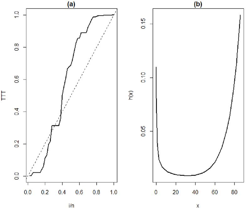
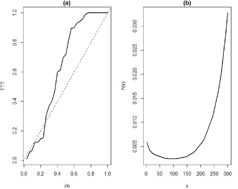
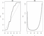
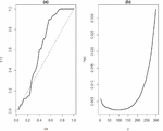
The data set is given by Aarset [21] and represents the time to first failure of 50 devices (in weeks). This data set is: 0.1, 0.2, 1, 1, 1, 1, 1, 2, 3, 6, 7, 11, 12, 18, 18, 18, 18, 18, 21, 32, 36, 40, 45, 46, 47, 50, 55, 60, 63, 63, 67, 67, 67, 67, 72, 75, 79, 82, 82, 83, 84, 84, 84, 85, 85, 85, 85, 85, 86, 86. As shown in Figure 4(a), the scaled TTT-Transform plot of this data set has a convex shape followed by a concave shape. So, the data set has a bathtub-shaped hazard rate.

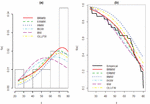
Table 3 gives the values of the MLEs of the parameters for all fitted distributions. Table 4 presents $-2\mathrm{\ell }$, AIC, BIC, CAIC, K-S statistics and the p-values of K-S test. The BRMW distribution has the smallest values for the $-2\mathrm{\ell }$, AIC, BIC, CAIC, K-S and highest p-value. So, the BRMW distribution gives an excellent fit than the others models for the Aarset data.

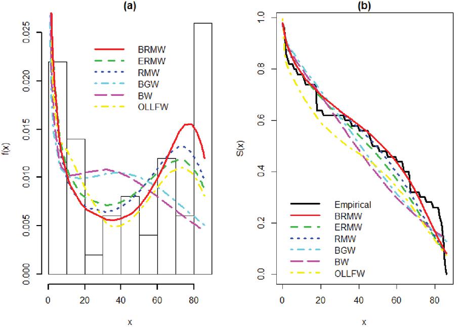
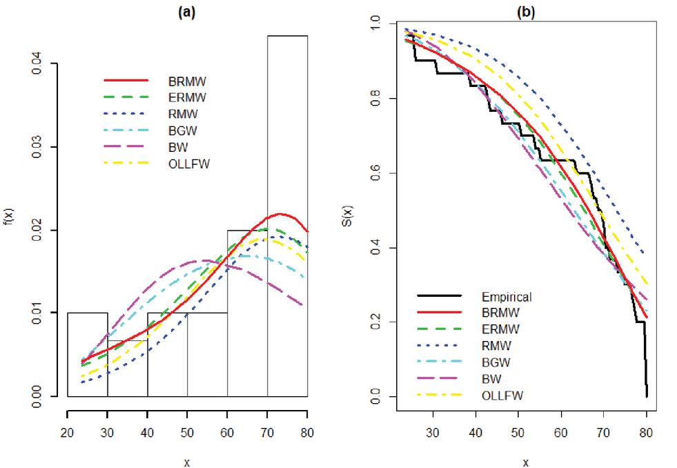
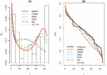
In addition, the plots of the estimated densities and the histogram of this data given in Figure 5(a) show that the BRMW pdf provides a closer fit to the histogram. The plots of the estimated and empirical survival function are displayed in Figure 5(b). These plots reveal that the survival function of the BRMW distribution is the closest curve to the empirical survival function. Figure 4(b) indicates that the estimated hazard function has a bathtub-shaped shape. The variance-covariance matrix for the estimated parameters of the BRMW distribution is given by

$J^{-1}(\widehat{\xi })=-\left(\begin{array}{c}\hfill \hfill \\ \hfill 0.2769\hfill & \hfill 0.0011\hfill & \hfill -0.0013\hfill & \hfill 0.0824\hfill & \hfill -0.0483\hfill \\ \hfill 0.0011\hfill & \hfill 0.00004\hfill & \hfill -0.0002\hfill & \hfill -0.0005\hfill & \hfill -0.0003\hfill \\ \hfill -0.0013\hfill & \hfill -0.0002\hfill & \hfill 0.00093\hfill & \hfill 0.0031\hfill & \hfill 0.0008\hfill \\ \hfill 0.0824\hfill & \hfill -0.0005\hfill & \hfill 0.0031\hfill & \hfill 0.1800\hfill & \hfill -0.0054\hfill \\ \hfill -0.0483\hfill & \hfill -0.0003\hfill & \hfill 0.0008\hfill & \hfill -0.0054\hfill & \hfill 0.0099\hfill \end{array}\right),$

So, the approximate $95\%$ confidence intervals for the parameters $\alpha ,\beta ,\lambda ,a$ and $b$ are (0.00;1.8412], (0.00;0.0153], [0.0212;0.1413], [0.3157;1.9793] and (0.00;0.3008] respectively.

Figure 4 (a) TTT-Transform plot and (b) BRMW hazard rate function for the Aarset data.

Table 3 MLEs and standard errors (in parentheses) of the model parameters for the Aarset data

Model	$\alpha$	$\beta$	$\lambda$	$a$	$b$
BRMW	0.8096	0.0017	0.0812	1.1475	0.1051
	(0.5263)	(0.0069)	(0.0306)	(0.4244)	(0.0998)
ERMW	0.0923	0.0022	0.0521	1.1340
	(0.0403)	(0.0063)	(0.0301)	(0.2626)
RMW	0.0746	0.0014	0.0575
	(0.0415)	(0.0128)	(0.0579)
BGW	0.0294	1.8812	0.0031	3.8281	0.1353
	(0.0086)	(0.5256)	(0.0066)	(0.0017)	(0.0804)
BW		1.5461	0.0350	0.2584	0.0530
		(0.9302)	(0.0775)	(0.1389)	(0.0204)
GOLLFW	0.0851	39.1352		0.0408	0.1577
	(0.0864)	(6.7242)		(0.0049)	(0.0058)

Table 4 The values of $-2\widehat{\mathrm{\ell }}$, AIC, BIC, CAIC and K-S with the corresponding p-values for the Aarset data

Model	$-2\widehat{\mathrm{\ell }}$	AIC	BIC	CAIC	K-S	p-value
BRMW	432.8562	442.8562	448.5043	443.7451	0.1239	0.4267
ERMW	439.6272	447.6272	455.2753	448.5161	0.1414	0.2703
RMW	437.9118	443.9118	449.6478	444.4335	0.1384	0.2939
BGW	462.3321	472.3321	481.8923	473.6958	0.1536	0.189
BW	464.5342	472.5342	480.1823	473.4231	0.1654	0.1298
GOLLFW	438.8676	446.8676	454.5157	447.7565	0.1501	0.2099

Figure 5 (a) Plots of the histogram and the fitted densities (b) empirical survival function and estimated survival functions for the Aarset data.

9.2 Data Set 2: Meeker and Escobar Data (Complete Data)

This data set is studied by Meeker and Escobar [22] and gives the times of failure and running times for a sample of 30 devices from a field-tracking study of a larger system. The data set is: 2, 10, 13, 23, 23, 28, 30, 65, 80, 88, 106, 143, 147, 173, 181, 212, 245, 247, 261, 266, 275, 293, 300, 300, 300, 300, 300, 300, 300, 300. The TTT-transform plot in Figure 6(a) shows that the data set exhibits a bathtub-shaped hazard rate.

The MLEs of the parameters of all models are given in Table 5 whereas the statistics $-2\mathrm{\ell }$, AIC, BIC, CAIC and K-S with the corresponding p-value are listed in Table 6. Since the values of $-2\mathrm{\ell }$, AIC, BIC, CAIC and K-S are smaller and the p-value is higher for the BRMW model when compared with those values of the other models, then the BRMW model gives the best fit for the data set.

Figure 6 (a) TTT-Transform plot and (b) BRMW hazard rate function for the Meeker and Escobar data.

Table 5 MLEs and standard errors (in parentheses) of the model parameters for the Meeker and Escobar data

Model	$\alpha$	$\beta$	$\lambda$	$a$	$b$
BRMW	0.3656	0.0024	0.0194	2.0632	0.1088
	(0.0317)	(0.0087)	(0.0162)	(0.8374)	(1.1155)
ERMW	0.0494	0.0019	0.0128	1.4480
	(0.0495)	(0.0104)	(0.0191)	(0.6681)
RMW	0.0491	0.0019	0.01300
	(0.0165)	(0.0042)	(0.0082)
BGW	14.9067	1.0637	0.0028	0.0682	18.8482
	(0.0004)	(0.1221)	(0.0020)	(0.0160)	(0.0001)
BW	1.4101	0.0107	0.4644	0.0490
	(0.0026)	(0.0794)	(0.0189)	(0.0053)
GOLLFW	0.2268	13.6617		0.0083	3.1641
	(0.1181)	(0.2993)		(0.0015)	(2.7306)

Table 6 The values of $-2\widehat{\mathrm{\ell }}$, AIC, BIC, CAIC, K-S and p-values for the Meeker and Escobar data

Model	$-2\widehat{\mathrm{\ell }}$	AIC	BIC	CAIC	K-S	p-value
BRMW	343.0634	353.0634	360.0694	355.5634	0.1456	0.5483
ERMW	347.7469	355.7469	361.3517	357.3469	0.1545	0.4714
RMW	351.5551	357.5551	361.7587	358.4782	0.2423	0.0591
BGW	361.0988	371.0988	378.1048	373.5988	0.2475	0.0507
BW	365.2835	373.2835	378.8883	374.8835	0.1927	0.2148
GOLLFW	351.7009	359.7009	365.3057	361.3009	0.2221	0.1034

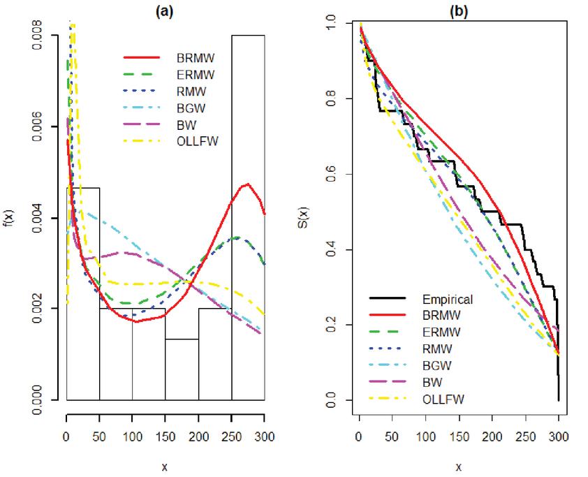
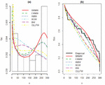
Figures 7(a) and 7(b) illustrate the pdfs and the empirical survival functions, respectively, of the comparative models to show the over fitting of the BRMW distribution. Figure 6(b) indicates that the estimated hazard function has a bathtub-shaped shape.

Figure 7 (a) Plots of the histogram and the fitted densities (b) empirical survival function and estimated survival functions for the Meeker and Escobar data.

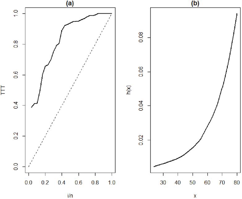
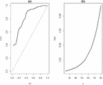
Figure 8 (a) TTT-Transform plot and (b) BRMW hazard rate function for the Aarset data.

The estimated variance-covariance matrix of the BRMW distribution is

$J^{-1}(\widehat{\xi })=-\left(\begin{array}{c}\hfill \hfill \\ \hfill 0.0010\hfill & \hfill -0.0002\hfill & \hfill 0.0003\hfill & \hfill 0.0192\hfill & \hfill 0.0079\hfill \\ \hfill -0.0002\hfill & \hfill 7.6\times {10}^{-5}\hfill & \hfill -0.0001\hfill & \hfill -0.0053\hfill & \hfill -0.0079\hfill \\ \hfill 0.0003\hfill & \hfill -0.0001\hfill & \hfill 0.0002\hfill & \hfill 0.0094\hfill & \hfill 0.0134\hfill \\ \hfill 0.0192\hfill & \hfill -0.0053\hfill & \hfill 0.0094\hfill & \hfill 0.7013\hfill & \hfill 0.6763\hfill \\ \hfill 0.0079\hfill & \hfill -0.0079\hfill & \hfill 0.0134\hfill & \hfill 0.6763\hfill & \hfill 1.2445\hfill \end{array}\right),$

So, the approximate $95\%$ confidence intervals for the parameters $\alpha ,\beta ,\lambda ,a$ and $b$ are, respectively, [0.3033;0.4279], (0.00;0.0196], (0.00;0.0512], [0.4217;3.7046] and (0.00,2.2953].

Table 7 MLEs and standard errors (in parentheses) of the model parameters for the Liu and Abeyratne data

Model	$\alpha$	$\beta$	$\lambda$	$a$	$b$
BRMW	0.3306	0.0029	0.0588	9.5612	0.4552
	(0.2812)	(0.0017)	(0.0138)	(12.4000)	(0.5074)
ERMW	0.0743	0.0172	0.0353	3.3595
	(0.0706)	(0.0147)	(0.0525)	(0.0019)
RMW	0.1036	0.2379	0.0113
	(0.0211)	(0.5578)	(0.0254)
BGW	15.7172	1.2452	0.0063	0.2002	12.92658
	(11.2279)	(0.0897)	(0.0042)	(0.1248)	(14.0341)
BW		1.1084	0.0139	5.6711	2.1871
		(0.2816)	(0.0121)	(2.7254)	(3.3199)
GOLLFW	3.6195	3.1609		0.0077	3.0137
	(3.1079)	(1.7824)		(0.0052)	(5.3605)

Table 8 The values of -2$\widehat{\mathrm{\ell }}$, AIC, BIC, CAIC, K-S and p-values for the Liu and Abeyratne data

Model	$-2\widehat{\mathrm{\ell }}$	AIC	BIC	CAIC	K-S	p-value
BRMW	225.4037	235.4037	242.4097	237.9037	0.21135	0.1371
ERMW	229.6155	237.6155	243.2203	239.2155	0.24179	0.05993
RMW	233.7462	239.7462	243.9498	240.6692	0.39603	0.0001638
BGW	226.9627	236.9627	243.9687	239.4627	0.22903	0.08593
BW	229.6841	237.6841	243.2889	239.2841	0.26052	0.03408
GOLLFW	229.0184	237.0184	242.6232	238.6184	0.30199	0.008406

9.3 Data Set 3: Liu and Abeyratne Data (Censored Data)

This data set is introduced by Liu and Abeyratne [23]. They supposed that the reliability of a certain mechanical component of an automobile is tested using an accelerated bench test. From Figure 8(b), we conclude that data set has an increasing hazard rate. So, the BRMW distribution is appropriate for modeling this data. The MLEs of the parameters of all models are given in Table 7. Table 8 shows that the BRMW distribution has the smallest values of the $-2\mathrm{\ell }$, AIC, BIC, CAIC, K-S and the highest p-value. So, the BRMW distribution provides the best fit than the others models. This result is confirmed in Figure 9. Figure 8(b) indicates that the estimated hazard function has an increasing shape. The estimated variance-covariance matrix of the BRMW distribution for the this data set is

$J^{-1}\left(\widehat{\xi }\right)=-\left(\begin{array}{c}\hfill \hfill \\ \hfill 0.0790\hfill & \hfill -0.0001\hfill & \hfill 0.0023\hfill & \hfill 3.0851\hfill & \hfill -0.1011\hfill \\ \hfill -0.0001\hfill & \hfill 2.9\times {10}^{-6}\hfill & \hfill -1.0\times {10}^{-5}\hfill & \hfill -0.0053\hfill & \hfill -1.2\times {10}^{-5}\hfill \\ \hfill 0.0023\hfill & \hfill -1.0\times {10}^{-5}\hfill & \hfill 1.9\times {10}^{-4}\hfill & \hfill 0.0465\hfill & \hfill -5.9\times {10}^{-3}\hfill \\ \hfill 3.0851\hfill & \hfill -0.0053\hfill & \hfill 0.0465\hfill & \hfill 153.761\hfill & \hfill -2.1121\hfill \\ \hfill -0.1011\hfill & \hfill -1.2\times {10}^{-5}\hfill & \hfill -5.9\times {10}^{-3}\hfill & \hfill -2.1121\hfill & \hfill 0.2574\hfill \end{array}\right),$

So, the approximate $95\%$ confidence intervals for the parameters $\alpha ,\beta ,\lambda ,a$ and $b$ are, respectively, (0.00;0.8818], (0.00;0.0063], [0.0318;0.0859], (0.00;33.8654] and (0.00;1.4499].

Figure 9 (a) Plots of the histogram and the fitted densities (b) empirical survival function and estimated survival functions for the Liu and Abeyratne data.

10 Conclusion

We have proposed a new five-parameter distribution, called the beta reduced modified Weibull distribution, which generalizes the reduced modified Weibull distribution discussed by Almalki [15]. We have seen that the proposed distribution exhibits a decreasing, increasing, bathtub, unimodal (upside-down bathtub) and modified unimodal shaped hazard rates. We have also seen that this distribution has a bathtub-shaped hazard rate function with a long flat region. Hence, it can be used to fit various types of data sets in reliability analysis. We have derived the algebraic expansions for the moments, quantile function, stress-strength reliability and the order statistics. We have estimated, for complete and censored data, the unknown parameters of new model by maximum likelihood method and obtained the observed information matrix. A simulation study proved that the maximum likelihood method performs well for estimating the parameters. We have shown, by means of three reliability data sets (complete and censored) that the new distribution is more flexible when it is compared to other modifications of the Weibull distribution.

Appendix

We present the following R code to compute the value of the pdf of BRMW distribution:

f=function(x,alpha,beta,lambda,a,b)
A=-(alpha*sqrt(x))-(beta*sqrt(x))*exp(lambda*x)
B=alpha+(beta*(1+2*lambda*x)*exp(lambda*x)
g=(1/(2*sqrt(x)))*B*exp(A)
G=1-exp(A)
ff=(1/beta(a,b))*g*(G$\wedge$(a-1))*((1-G)$\wedge$(b-1)) return(ff)

The R code to compute the moments of BRMW distribution:

moment=function(alpha,beta,lambda,a,b,r)
ff=function(x,alpha,beta,lambda,a,b,r)
(x$\wedge$r)*(f(x,alpha,beta,lambda,a,b))
mr=integrate(ff,lower=0,upper=Inf,subdivisions=100,
alpha=alpha,beta=beta,lambda=lambda,a=a,b=b,r=r)
return(mr)

The R code to generate random variables from BRMW distribution with $\alpha \mathrm{=}\mathrm{2.5}\mathrm{,}\beta \mathrm{=}\mathrm{0.5}\mathrm{,}\lambda \mathrm{=}\mathrm{1.5}\mathrm{,}a\mathrm{=}\mathrm{4}$ and $b\mathrm{=}\mathrm{3.5}$ :

n=seq(1,100,1)
alpha=2.5;beta=0.5;lambda=1.5;a=4;b=3.5
T=function(x)alpha*sqrt(x)+beta*sqrt(x)*exp(lambda*x)
inverse=function(v,lower,upper)
uniroot((function(x)
T(x)+log(1-v)),lower=lower,upper=upper)$root
Xgenerator=function(n,lower,upper)
V=rbeta(n,4,3.5)
X=c()
for(i in 1:n)
X[i]=inverse(V[i],lower,upper)
return(X)

The R code to obtain the MLEs of BRMW distribution parameters:

x=c(X)  X is the data set
LikFunf=function(alpha,beta,lamda,a,b)
A=-(alpha*sqrt(x))-(beta*sqrt(x))*exp(lambda*x)
B=alpha+(beta*(1+2*lambda*x)*exp(lambda*x))
g=(1/(2*sqrt(x)))*B*exp(A)
G=1-exp(A)
log=-sum(-log(beta(a,b))+log(g)+(a-1)*log(G)+(b-1)*log(1-G))
return(log)
mle.results=mle2(LikFunf,start=list(alpha=alpha,beta=beta,
lambda=lambda,a=a,b=b),hessian.opts=TRUE)
summary(mle.results)

We obtain the variance covariance matrix of BRMW distribution by:

vcov(mle.results)

The R code to compute the value of Bias and RMSE with N iterate and sample size n (for example for alpha parameter):

N=5000
n=c(50,100,200,300,500)
for(i in 1:length(n))
for(j in 1:N)
x=Xgenerator(n[i],-1000,1000)
alphamle[j]=coef(mle.results)[1]
bias1alpha[j]=alphamle[j]-alpha
RMSE1alpha[j]=sqrt((bias1alpha[j])$\wedge$2)
biasalpha[i]=mean(bias1alpha)
RMSEalpha[i]=mean(RMSE1alpha)

References

[1] C.D. Lai, M. Xie and D.N.P. Murthy. A modified Weibull distribution. EEE Transactions on Reliability, 52(1):33-37, 2003.

[2] M. Bebbington, C.D. Lai, and R. Zitikis. A flexible Weibull extension. Reliability Engineering and System Safety, 92:719-726, 2007.

[3] A.M. Sarhan and J. Apaloo. Exponentiated modified weibull extension distribution. Reliability Engineering and System Safety, 112:137-144, 2013.

[4] F. Famoye, C. Lee and O. Olumolade. The beta-Weibull distribution. Journal of Statistical Theory and Applications, 4(2):121-136, 2005.

[5] L. Benkhelifa. The Weibull Birnbaum-Saunders distribution and its applications. Statistics, Optimization and Information Computing, 9(1):61-81, 2021.

[6] W. Nelson. Accelerated life testing: statistical models. data analysis and test plans. New York: Wiley; 1990.

[7] G.O. Silva, E.M. Ortega and G.M. Cordeiro. The beta modified Weibull distribution. Lifetime Data Analysis, 16(3):409-430, 2010.

[8] G.M. Cordeiro, E.M. Hashimoto and E.M. Ortega and . The McDonald Weibull model. Statistics, 48(2):256-278, 2014.

[9] N. Singla, K. Jain and S. Kumar Sharma. The beta generalized Weibull distribution: properties and applications. Reliability Engineering and System Safety, 102:5-15, 2012.

[10] A. Saboor, H.S. Bakouch and M.N. Khan. Beta Sarhan–Zaindin modified Weibull distribution. Applied Mathematical Modelling, 40: 6604, 2016.

[11] B. He and W. Cui. An additive modified Weibull distribution. Reliability Engineering and System Safety, 145:28-37, 2016.

[12] F. Prataviera E.M. Ortega, G.M. Cordeiro, R.R. Pescim and B.A.W. Verssania. A new generalized odd log-logistic flexible Weibull regression model with applications in repairable systems. Reliability Engineering and System Safety, 176:13–26, 2018.

[13] A.A. Ahmad and M.G.M. Ghazal. Exponentiated additive Weibull distribution. Reliability Engineering and System Safety, 193:106663, 2020.

[14] S.J. Almalki and J. Yuan. The new modified Weibull distribution. Reliability Engineering and System Safety, 111:164-170, 2013.

[15] S.J. Almalki. Reduced new modified Weibull distribution. Communications in Statistics - Theory and Methods, 47:2297-2313, 2018.

[16] W. Kuo and M.J. Zuo. Reduced new modified Weibull distribution. Optimal reliability modeling: principles and applications. Wiley; 2001.

[17] N. Eugene and F. Famoye. Beta-normal distribution and its applications. Communications in Statistics - Theory and Methods, 31:497-512, 2002.

[18] B.C. Arnold and H.N. Nagarajah. A first course in order statistics. New York: John Wiley, 2008.

[19] I.S. Gradshteyn and I.M. Ryzhik. Table of integrals, Series and Products. Academic Press, New York; 2000.

[20] R.G. Miller, G. Gong and A. Muñoz. Survival analysis. New York: John Wiley and Sons; 1981.

[21] M.V. Aarset. How to identify a bathtub hazard rate. EEE Transactions on Reliability, 36(1):106-108, 1987.

[22] W.Q. Meeker and L.A. Escobar. Statistical methods for reliability data. New York: Wiley; 1998.

[23] Y. Liu and A.I. Abeyratne. Practical applications of bayesian reliability. New York: John Wiley and Sons; 2019.

Biography

Lazhar Benkhelifa received the engineer degree in statistics from university of Biskra (Algeria), the Magister degree in probability and statistics from university of Biskra (Algeria), the doctorate degree in statistics from university of Biskra (Algeria) in 2015 and the habilitation (Habilitation Universitaire) from university of Oum El Bouaghi (Algeria) in 2018. He works as a teacher at the department of Mathematics and Informatics, Larbi Ben M’Hidi University, Oum El Bouaghi, Algeria. His current research activities are focused in the following aspects: statistical computing, Life time data analysis, distribution theory and statistical software.

Journal of Reliability and Statistical Studies, Vol. 14, Issue 1 (2021), 311–322.
doi: 10.13052/jrss0974-8024.14115
© 2021 River Publishers